Abstract
Measuring interpupilary distance and pupil height is a crucial step in the process of optometry. However, existing methods suffer from low accuracy, high cost, a lack of portability, and limited research on studying both parameters simultaneously. To overcome these challenges, we propose a method that combines ensemble regression trees (ERT) with the BlendMask algorithm to accurately measure both interpupillary distance and pupil height. First, we train an ERT-based face keypoint model to locate the pupils and calculate their center coordinates. Then, we develop an eyeglass dataset and train a BlendMask model to obtain the coordinates of the lowest point of the lenses. Finally, we calculate the numerical values of interpupillary distance and pupil height based on their respective definitions. The experimental results demonstrate that the proposed method can accurately measure interpupillary distance (IPD) and pupil height, and the calculated IPD and pupil height values are in good agreement with the measurements obtained by an auto-refractometer. By combining the advantages of the two models, our method overcomes the limitations of traditional methods with high measurement accuracy, low cost, and strong portability. Moreover, this method enables fast and automatic measurement, minimizing operation time, and reducing human errors. Therefore, it possesses broad prospects for application, particularly in the fields of eyeglass customization and vision inspection.
1. Introduction
The human eye plays a crucial role not only in daily life but also as one of the key features of humans. Eye tracking has a wide range of applications in various fields, such as medical research (psychology, cognition) [1,2,3], electronic games [4], and human-computer interaction [5]. Among these, one of the most significant areas of research is ophthalmology. In recent years, the problem of myopia has become increasingly severe, with a growing number of individuals needing to wear corrective glasses. Spectacles are optical devices that operate based on the principle of light refraction [6]. They are used to correct refractive errors by placing a lens of a specific size in front of the eyes. Refractive errors occur when an object does not properly focus on the retina. One of the measurements taken during the spectacle dispensing process is the alignment measurement of the pupillary distance (PD), pupillary height (PH), and optical center (OC) [6] of the lens. Therefore, research on accurate measurements of pupillary distance and height is of great significance.
Pupillary distance (PD), defined as the distance between the centers of the two pupils [7], and pupillary height (PH), which refers to the distance from the center of the pupil to the lowest point on the lower rim of the frame measured along the visual axis of the eye passing through the lens, are essential measurement parameters in the fields of ophthalmology and optometry, commonly expressed in millimeters. In Figure 1a, the variables “dlc” and “drc” represent the left and right interpupillary distances, respectively. The sum of these distances is referred to as the total PD. Similarly, “hl” and “hr” represent the left and right pupil heights, respectively. These parameters can be utilized in various aspects, such as optometric fitting, customization of eyeglasses, and vision correction. However, inaccurate measurement of PD or PH, or a mismatch between the optical center of the lens and the PD, can cause distorted, blurred, and ambiguous visual images, leading to visual fatigue and damage to the eyes. There have been numerous studies on the importance of PD, including potential applications in biological characteristics.
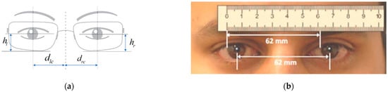
Figure 1.
Definition and manual measurement. (a) Definition of pupillary distance and height. (b) Manual measurement using a ruler.
Traditionally, pupillary distance and height measurements have been obtained through manual measurement using rulers by optometrists in the design and manufacturing of eyeglasses, as shown in Figure 1. While this method is convenient and simple, it is prone to significant errors and can be easily influenced by human factors. Modern glasses accommodate far, intermediate, and near vision corrections in the same pair, making the precision requirements even more demanding. To achieve high precision levels, lens manufacturers have developed systems to measure pupil distance to one millimeter or below in error tolerance. This method is called photographic measurement [8], which involves using a camera to capture images of the eye and calculating the pupillary distance based on the size and position of the pupils in the images. The method is more precise but requires manual measurement as well as consideration of factors such as camera distance and angle. With the advancement of technology, a virtual measurement method [9] can also be used by constructing a 3D model of the eye using virtual reality technology, which is not limited by equipment or environmental constraints and can measure multiple parameters. However, this method requires professional software and technical support, and it can be expensive and infeasible for many individuals, while visual impairment affects a large number of people worldwide.
Existing methods to measure pupillary distance often have limitations and cannot measure pupillary height. A practical solution would be to use portable devices such as cellphones and tablets since heavy equipment is not portable and sophisticated technologies remain inaccessible to many. Embedded micro-optics in phones constantly improve, and algorithms for pupil distance measurement can be integrated into applications. With advancements in computer vision and machine learning technology, it is now possible to automatically and accurately measure pupillary distance using computers or mobile devices. By utilizing computer vision and machine learning techniques to process and analyze eye images, automatic measurement of pupillary distance can be achieved. This method is fast, highly accurate, and stable, significantly reducing the need for human and material resources and improving the portability of measuring pupillary distance and height during eyeglass fitting. Therefore, we will conduct our research from the following directions:
- (1)
- Capture facial images and process them using image processing techniques;
- (2)
- Use integrated regression tree algorithms to locate the pupils;
- (3)
- Use the BlendMask algorithm to locate the eyeglass frames;
- (4)
- Calculate the pupil distance and height based on defined parameters;
- (5)
- Integrate the above steps into a single model for simultaneous measurement of pupil distance and height;
- (6)
- Compare the values of pupil distance calculated by our model with those measured by a ruler and an auto-refractometer, and analyze the consistency among the three measurement methods.
The primary focus of our study is to research measurement methods for pupil distance and pupil height, and compared with existing approaches, the main contributions of this research are as follows. We propose a method that combines ensemble regression trees with the BlendMask algorithm, which can be integrated into devices such as smartphones and computers, enabling simultaneous and automated measurements of interpupillary distance and pupil height. Furthermore, the method we propose offers numerous advantages, including high precision, ease of operation, non-contact measurement, low cost, and rapid measurement. Our method empowers users to provide measurement results to online eyewear retailers, facilitating eyeglass fitting services at home without the need to visit physical eyewear stores. Through continued research and improvement, our goal is to provide an accurate, convenient, and practical method for measuring pupil distance and pupil height, addressing the needs of eyewear wearers and related fields.
This section provides an explanation of pupil distance and height definitions, summarizes existing methods for measuring pupil distance, and briefly introduces the objectives of this study. The remainder of the article is organized as follows. Section 2 provides a brief summary of related work relevant to this research. Section 3 then provides a detailed description of the work carried out in this study, followed by Section 4, which describes the experiments, results, and discussion. Finally, Section 5 presents the conclusions and limitations of the proposed method, along with suggestions for further research.
2. Related Works
Our research primarily focuses on measuring interpupillary distance and pupil height. The accurate determination of the position of the pupil is essential for interpupillary distance measurement. Pupil detection techniques have been widely employed across various fields and have become a prominent subject of international research. Conversely, there is relatively limited research on pupil height measurement. In the context of pupil height measurement, accurately obtaining the lowest point of eyeglass lenses is crucial. This requires not only determining the position of the lenses but also assessing their size to subsequently calculate the position of the lowest point. Therefore, we employed an instance segmentation approach to locate the eyeglass lenses and measure their size. Throughout the entire process, we primarily utilized techniques related to pupil detection and instance segmentation.
2.1. Pupil Detection Technology
In recent years, there has been an increase in the development of methods for detecting the center of the pupil using both traditional image processing techniques and machine learning-based approaches. Various algorithms for locating the eyes have been proposed, including the typical anthropometry-based method using standard measurements [10], the skin color model-based detection method [11], and statistical learning methods based on training data [12]. Among these, the statistical learning algorithm-based method is particularly popular in the current field of eye detection due to its high applicability and potential for further exploration in the areas of artificial intelligence and pattern recognition. The primary statistical learning algorithms used for eye detection are the AdaBoost algorithm [13] and the deep learning algorithm [14], both of which have demonstrated promising results in the field of human eye measurement.
Wen-Cheng Wang and Liang Chang [15] proposed a region projection-based method for eye localization that calculates two-dimensional features during the projection process and locates the eye pupil through boundary tracking of the grayscale characteristics. However, this method is easily affected by the results of face measurement and does not consider individual differences in facial features, resulting in imprecise localization. Kumar et al. [16] used a hierarchical search space reduction technique to locate the pupil region by distinguishing the color difference between the face skin and the eye color. This method mainly uses the color information of the face image to locate the eyes but is also highly affected by external factors and has weak adaptability. With the development of machine learning technology, more attention has been paid to the use of machine learning for eye recognition. Yan Wu, Yang Yang, et al. [17] proposed a precise pupil localization method based on a neural network, which uses a gray-scale histogram for rough localization and a BP neural network for accurate pupil localization. This method showed good performance in experiments, but its accuracy needs to be improved on complex backgrounds. Gao-Feng Xu et al. proposed a joint eye localization method [18], which uses edge histograms as classification features and cascaded classifiers based on the AdaBoost algorithm, achieving good experimental results. Overall, these studies demonstrate the potential of machine learning-based methods for accurate and robust pupil detection. However, there is still room for improvement in terms of generalization to diverse conditions, computational efficiency, and adaptability to different hardware platforms.
Vahid Kazemi and Josephine Sullivan [19] presented a method for estimating facial landmark positions directly from a sparse subset of pixel intensities using an ensemble of regression trees. They proposed a gradient-boosting algorithm based on learning a collection of regression trees that can accurately identify the key points of the face. Based on this algorithm, we optimized the parameters and trained a facial key point detection model, which demonstrates a high degree of accuracy in locating the pupils.
2.2. Instance Segmentation Algorithm
Object detection, or localization, is a crucial step in the progression from coarse to fine digital image inference. It not only provides the classes of the image objects but also provides the location of the image objects that have been classified.
Instance segmentation is a challenging and important area in machine vision research that aims to predict object class labels and pixel-specific object instance masks to localize different classes of object instances in various images. This field has many applications in robotics, autonomous driving, and surveillance. With the advent of deep learning [20], specifically convolutional neural networks (CNNs) [21,22], many instance segmentation frameworks have been proposed, such as Mask R-CNN [23], which uses a fully convolutional network (FCN) [24,25] to predict segmentation masks alongside box regression and object classification. To improve performance, the feature pyramid network (FPN) [26] has been used to extract stage-wise network features, and new datasets such as Microsoft’s COCO dataset [27], the Cityscapes dataset [28], and the Mapillary Vistas Dataset (MVD) [29] have provided opportunities for improving proposed techniques. Network design principles for image classification have also been proposed and are useful for object recognition, including shortening information paths, using dense connections, and increasing information path flexibility and diversity by creating parallel paths. Although there are numerous techniques applied to instance segmentation, notable methods are highlighted in the timeline presented in Figure 2.
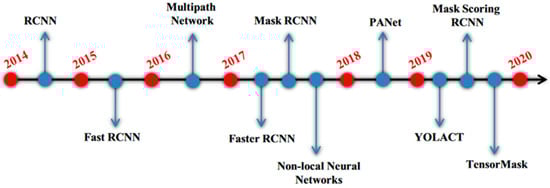
Figure 2.
Timeline for notable techniques in instance segmentation [30].
In 2020, Hao Chen et al. [31] proposed a new instance segmentation algorithm called BlendMask, which combines the algorithmic ideas of Mask R-CNN and YOLACT and introduces a novel Blender module. The model achieves state-of-the-art performance, with a highest accuracy of 41.3 AP, while the real-time version, BlendMask-RT, achieves a performance of 34.2 mAP and a speed of 25 FPS, both surpassing Mask R-CNN. Based on this algorithm, we perform the localization and size measurement of eyeglass lenses.
3. Methods
3.1. Dataset Collection and Preprocessing
The 300 W [32] dataset is the most widely used outdoor dataset and contains five face datasets (LFPW, AFW, HELEN, XM2VTS, and IBUG), with 68 landmarks per image. The annotation distribution is shown in Figure 3. In the 300 W dataset, there are 3148 training samples and 689 testing samples. Furthermore, the training set can be further divided into the common subset and the challenge subset. The Common subset (LFPW and HELEN) has a total of 554 test images, while the challenge subset (IBUG) includes 135 images.
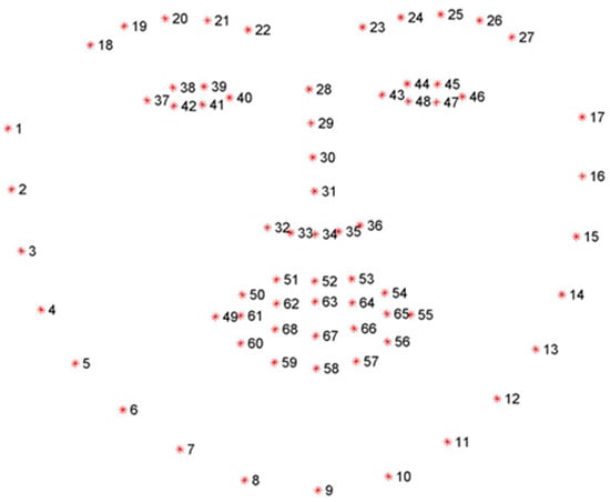
Figure 3.
Sixty-eight key points of the human face.
As per the experimental requirements, we utilized the LabelMe tool to precisely label the various parts of the eyeglasses. Upon labeling, a corresponding JSON file was generated for each image. Subsequently, these JSON files underwent processing to generate trainable data for the experiments.
Image semantic segmentation requires precise data labeling, which is time-consuming and labor-intensive. Moreover, experiments often lack sufficiently high-quality labeled data samples. Therefore, default data augmentation methods are adopted to expand image samples, mainly through flipping, cropping, etc. On the one hand, this increases the number of experimental samples, and on the other hand, it prevents overfitting.
3.2. Pupil Location
Vahid Kazemi and Josephine Sullivan [19] proposed a method to estimate facial landmark positions directly from a sparse subset of pixel intensities using an ensemble of regression trees. Based on a gradient boosting framework, the ensemble of regression trees is trained to optimize the sum of squared error loss and naturally handles missing or partially labeled data. We used a two-layer regression to build the mathematical model.
3.2.1. Training of the First-Layer Regression
In this layer, the training dataset is used as input, where represents the image and represents the position of facial landmarks. The method [19] of regression variable cascade is adopted, where the prediction of each regressor in the cascade is based on the current image and the previous predicted position of landmarks . The iterative formula is expressed as:
in this regression training, represents the position of facial landmarks, represents the cascade number, and is the difference between the true value and the regression prediction result. In this regression training, the data can be organized in a triple array, where represents the image in the dataset. By iterating in this way, a set of regression models can be generated to obtain the required regression model.
3.2.2. Training of the Second-Layer Regression
The gradient boosting tree algorithm is used to train each regression model , with as the loss function and as the gradient. A learning parameter is set in the algorithm to help prevent overfitting. As shown in Figure 4, the process diagram illustrates the learning of “” in the cascade.
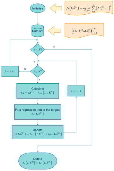
Figure 4.
The algorithm for learning in the cascade.
3.3. The Network Structure of BlendMask
BlendMask is a one-stage dense instance segmentation method that combines the concepts of top-down and bottom-up methods. It adds a bottom module on the basis of the anchor-free detection model FCOS [33] to extract low-level detailed features and predict an attention mechanism at the instance level. Hao Chen et al. drew inspiration from the fusion methods of FCIS [34] and YOLACT [35] and proposed the Blender module to better integrate these two types of features.
The architecture of BlendMask, which includes a detector module and a BlendMask module, is illustrated in Figure 5. FCOS is the detector module used in the paper. The BlendMask module consists of three components: the bottom module, which extracts low-level features and generates a score map known as base; the top module, which connects to the box head of the detector and generates top-level attention corresponding to base; and the blender, which combines base and attention.
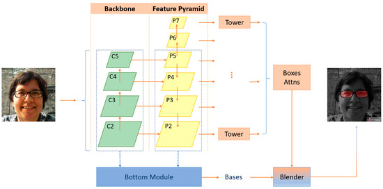
Figure 5.
BlendMask network structure.
3.3.1. Top-Layers
The main structure is the FCOS object detection model. The multi-level features output by FPN are used for both conventional object detection, obtaining a bbox and cls score, and generating spatial attention by being connected to conv. towers.
Based on the FCOS object detection model, the multi-level features output by FPN are used for both conventional object detection (obtaining bbox and cls scores) and generating spatial attention by being connected to conv. towers. The spatial attentions have a shape of . Each pixel location’s spatial attention belongs to a 3D structure: . This represents the embedding dimension of the per-pixel score map predicted by the bottom module, where represents the 2D spatial dimension of the attention (usually with a value of 4 or 8), indicating the ability of spatial attention to capture instance-level information, such as the pose and rough shape of the object.
The top-layers sort the bbox and attention of different objects based on their cls score, selecting the top D proposals, which are then applied to the information fusion process of the blender to obtain the top D box predictions P and their corresponding attentions A:
3.3.2. Bottom Module
This part of the structure is similar to FCIS and YOLACT, with the input being the low-level features of , which can come from either the backbone network’s low-level features (such as C2 and C3) or the feature pyramid network’s low-level features (such as P2 and P3), or even a fusion of both. Through a series of decode operations (upsampling and convolution), score maps are generated and referred to as the Base (B). In the equation above, N is the batch size, K is the number of Base maps, H and W are the input image sizes, and s is the output stride of the Base maps. This module is mainly used to obtain multiple masks for the entire image, which can be combined to generate a perfect mask. In this experiment, the architecture of the low-level branch adopts the decoder architecture of DeepLabV3+ [36], and it can be seen in Figure 6. Considering that the low-level branch is used to predict global semantic information, other similar dense prediction modules can theoretically be used as the architecture for the low-level branch.
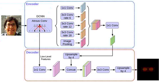
Figure 6.
DeepLabV3+ structure.
3.3.3. Blender Module
Blender is the core module of BlendMask, which combines position-aware attention information to generate the final prediction results. Its inputs include the bottom-level Base B, selected top-level attentions A, and bbox proposals P generated by the detector tower.
First, the ROIPooler of Mask R-CNN is used to extract the region of interest (ROI) corresponding to each proposed bounding box (bbox) from the base feature map. The ROI is then resized to a feature map of size :
As the size of the attention map is , which is smaller than , upsampling interpolation is applied to the attention map . Then, softmax normalization is performed along the K-dimension to obtain the attention weight map:
Finally, the score map and feature map are element-wise multiplied and added together, and then the resulting values are summed across channels to obtain the final mask.
3.3.4. Loss Function Design
In this work, we improved the original algorithm’s loss function and designed a loss function suitable for instance segmentation. The loss function was designed based on the localization output of object detection and the segmentation output of masks and is denoted as follows:
as shown in the formula, is the classification loss function, is the bounding box localization loss function for object detection, and is the loss function for mask segmentation. and are used to balance the relationship between the losses, and their values are both set to 1 in the experiments conducted in this study.
3.4. Head Pose Estimation
In computer vision, the pose of an object refers to its relative orientation and position in relation to a camera. This pose can be altered by either moving the object with respect to the camera or by moving the camera with respect to the object. In 3D space, the rotation of an object can be represented by three Euler angles (α, β, and γ), where α represents the yaw angle, β represents the roll angle, and γ represents the pitch angle of the head pose, as shown in Figure 7.
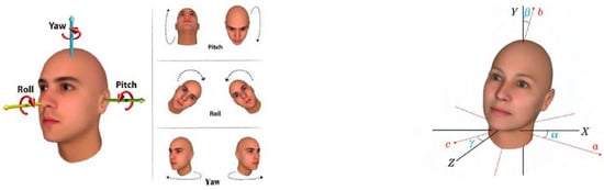
Figure 7.
Head Euler angles diagram.
To achieve head pose estimation, the algorithm [37] we adopt generally follows the steps shown in Figure 8. Firstly, an ensemble regression tree algorithm is used to train a model for extracting facial feature positions. These feature positions include key points on the face, such as the eyes, nose, and mouth. Next, the extracted facial feature positions are matched with the corresponding 3D face model, establishing the correspondence between the 3D facial feature points and the 2D facial images. Then, the PNP algorithm in OpenCV is utilized to solve the transformation relationship between the 3D facial feature points and the 2D facial images. Through this transformation relationship, we can obtain information about the head pose. Finally, with the help of rotation matrices, the Euler angles of the head pose can be calculated.
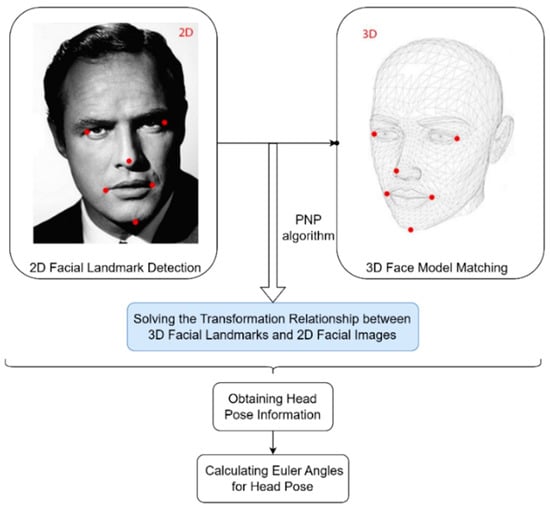
Figure 8.
Flowchart of head pose estimation Algorithm.
3.5. The Calculation of Pupil Distance and Pupil Height
3.5.1. Calculation Method of Pupil Distance
The pupil distance can be calculated based on the 68 facial landmarks. Specifically, we select four points (38, 39, 41, and 42) around the left eye and four points (44, 45, 47, and 48) around the right eye. The coordinates of these points are used to calculate the center coordinates of the left and right pupils. Suppose the coordinates of these four points are , the geometric center coordinates can be obtained by computing their average. The calculation formula is as follows:
thus the coordinates of the center of the left pupil and the center of the right pupil can be obtained. In two-dimensional space, the distance formula between two points can be used to calculate the interpupillary distance.
3.5.2. Calculation Method for Pupil Height
By using the BlendMask algorithm, the position of the glasses lens can be detected and the coordinates of its lowest point can be found. Then, the pupil height can be calculated as the vertical distance between the center of the pupil and the lowest point of the lens, rather than the Euclidean distance. Specifically, the formula is as follows:
4. Experimentation and Discussion
4.1. Experimental Environment
The programming language used in this experiment is Python, with PyTorch version 1.6.1 and CUDA version 10.1. PyTorch, an open-source deep learning framework, was utilized for building the deep neural network layers, while PyCharm was employed as the programming software. Related configurations are set out in Table 1.

Table 1.
Related configurations.
4.2. Program Measurement Process
The core of the program consists of two parts: the first part is facial keypoint detection, which aims to obtain the coordinates of the pupils; the second part is to recognize the position and size of the glasses lenses, with the goal of obtaining the coordinates of the lowest point of the lenses. By combining these two parts, the program can calculate the interpupillary distance and the pupil height. Considering the impact of head pose on the results, after obtaining the facial landmarks, we calculate the head pose information and assess whether the Euler angles of the head pose fall within the predefined threshold. If the Euler angles are within the specified threshold, it indicates that the head pose is suitable for measurement, and we can proceed to obtain the measurement results. However, if the Euler angles are outside the threshold range, it indicates that the head pose is not suitable for measurement and we need to retake the facial photo. The flowchart of the entire program can be seen in Figure 9.
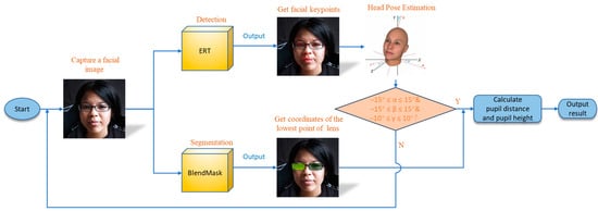
Figure 9.
Program flow chart.
4.3. Pupil Positioning Detection Results
The first method used is ensemble regression trees, which use a weighted average method during the training process to integrate the outputs of multiple regression trees to obtain more accurate facial keypoint localization results. The training parameters are shown in Table 2.
Table 2.
The training parameters.
This article conducted experiments to detect 68 key points on human faces, and some of the results are shown in Figure 10, which demonstrates the pixel coordinates of these 68 points in the image.
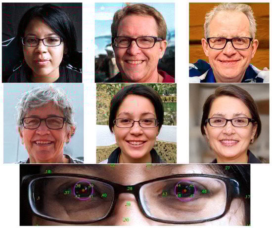
Figure 10.
The results of keypoint localization.
During testing, we observed that if the situation depicted in Figure 11a occurs, the pupil detection method may fail. As a result, we request that users look directly at the camera during testing. However, in the scenario shown in Figure 11b, even with a lateral gaze, the pupil can still be detected, although some degree of error may be present.
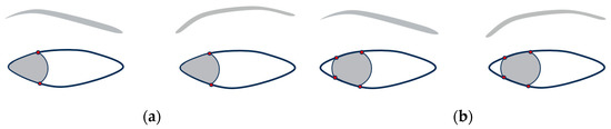
Figure 11.
Case of crossed eyes. (a) Completely oblique. (b) Partially oblique.
4.4. Glasses Lens Detection Results and Analysis
4.4.1. Training and Evaluation
The loss curve provides an intuitive way to assess the training progress and convergence of a neural network. In order to demonstrate the effectiveness of the model in a more intuitive way, this article used the TensorBoard visualization tool to record the details of the model’s learning during the training process and plotted the relationship between iteration number and test set loss, as shown in Figure 12. During the experiment, a total of five loss curves were recorded, including: loss_basis_sem, loss_focs_cls, loss_fcos_loc, loss_mask, and the final total_loss curve. Among them, the loss_focs_cls curve evaluates the model’s classification performance, which can show the specific details of the classification training process. The loss_fcos_loc curve evaluates the degree of position offset of the target detection box, where larger offsets correspond to higher loss values. The loss_mask curve evaluates the effect of pixel-wise segmentation of the image during instance segmentation. The total_loss curve is the sum of loss_basis_sem, loss_focs_cls, loss_fcos_loc, and loss_mask, which can provide a comprehensive evaluation of the overall performance.
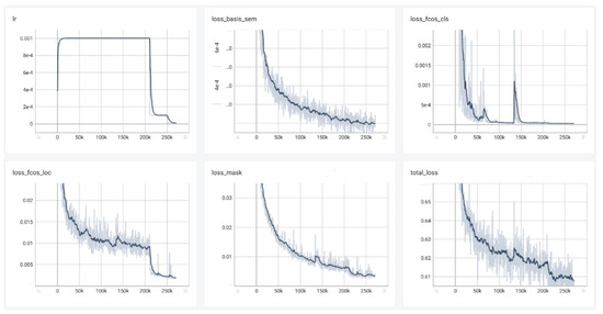
Figure 12.
The loss value changes with the training steps.
In order to evaluate the algorithm’s ability to recognize and determine the position of the glasses lenses, we used seven key metrics: precision rate (P), recall rate (R), metric function (F1), intersection over union (IOU), average precision (AP), mean average precision (mAP), and mean intersection over union (mIOU). Precision rate (P) represents how many true positive samples were correctly predicted among all samples predicted as positive, while recall rate (R) represents how many true positive samples were correctly predicted among all actual positive samples. The precision rates (P) and recall rates (R) can be defined as follows:
where “true positive (TP)” and “false positive (FP)” indicate the number of positive and negative results detected as positive, respectively, and “false negative (FN)” indicates the number of positive results detected as negative. The metric function (F1) of the precision and recall rates can be defined as follows:
To more extensively evaluate the model algorithm, the intersection over union error (IOU) was considered to examine the measurements. The detection performance of the model is evaluated considering the mean accuracy (mAP) [38]. The mAP can clearly reflect the performance when it is related to the target position information and category in the image. The IOU and mAP were defined as follows:
4.4.2. Results Show
With the BlendMask model we trained, we can accurately predict the position and size of glasses lenses in facial images and obtain the coordinates of the lowest point of the lenses. To directly display the algorithm detection results, we selected some images for illustration, as shown in Figure 13. From the figure, it can be seen that the model has excellent recognition ability for glasses, and the most important thing is that the mask area is accurately located.
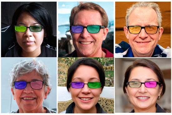
Figure 13.
The results of glasses lens detection.
4.5. Visualization of Head Pose Estimation
Due to the significant impact of head tilt on the measurement of interpupillary distance and pupil height, we need to determine whether the head is tilted in the images obtained by the user. For this purpose, we have adopted a head pose estimation algorithm based on the conversion of 2D facial landmark points to 3D. We selected 15 different angle photos of an individual, ran the trained head pose estimation algorithm, and then compared the algorithm’s estimated head pose with the actual pose. Experimental results indicate that, in most cases, this algorithm can accurately determine whether the head is tilted in the image and can estimate the tilt angle. The visualization of the head pose estimation process is shown in Figure 14.
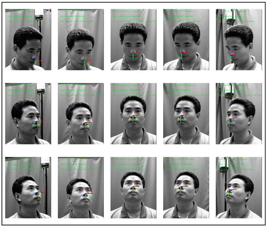
Figure 14.
Fifteen pose angles of an object.
After obtaining the head pose information, we conducted tests to assess the influence of head tilt angles on the measurement results of interpupillary distance and pupil height. To ensure acceptable accuracy, we set the following thresholds.
If −15° ≤ α ≤ 15°, −15° ≤ β ≤ 15°, and −10° ≤ γ ≤ 10°, then our measurement results are considered within an acceptable range of errors; otherwise, the measurement is not considered reliable. Here, α, β, and γ represent the yaw angle, roll angle, and pitch angle of the head pose, respectively. With this judgment condition, we can obtain more accurate and reliable measurement results while ensuring that the head pose is suitable for measurement. This processing approach effectively avoids the interference of head pose on the measurement results, thereby enhancing the accuracy and reliability of the measurements.
4.6. Measurement Results of Interpupillary Distance and Pupillary Height
To evaluate the effectiveness of our research, we recruited a total of 30 diverse participants for testing. The selection of participants was done randomly, without any restrictions based on age, gender, or race. Each participant was instructed to capture facial images using the same equipment. During the image capture process, we ensured ample lighting conditions and had participants seated in designated chairs to minimize movement. A tripod was positioned approximately 30 cm in front of each participant at eye level to hold a smartphone. The smartphone’s camera was aligned with the participant’s eyes. Participants were instructed to gaze directly at the smartphone’s camera on the tripod without closing or tilting their eyes, avoiding any special circumstances. In addition to using our method for testing, we also employed traditional ruler-based measurement of PD and an auto-refractometer (AU) for PD measurements. These additional measurement methods will be used for comparison and analysis along with our research results. The final measured experimental results can be found in Table 3.
Table 3.
Comparison of this development system with ruler measurement and auto-refractometer pupil distance measurement results.
In order to compare the differences among three different measurement methods, we generated a line graph (Figure 15) to plot the data from the three groups. From the graph, it can be observed that there is no significant difference among the data obtained from these three different measurement methods. Additionally, we conducted a repeated measurement variance analysis based on the measured data. Thirty testers used rulers to measure the pupillary distance (), used AU to measure the pupillary distance (), and used the model proposed in this paper to measure the pupillary distance (). The Greenhouse–Geisser correction estimated value for deviation from sphericity is denoted as . Our results indicate that there is no significant difference between the pupillary distance measured using the model proposed in this paper and that measured using rulers or AU, . Therefore, we conclude that the results of using the model proposed in this paper to measure the pupillary distance are accurate.
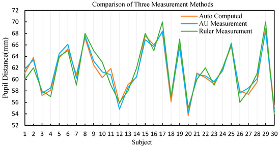
Figure 15.
Line graph comparing the three measurement methods.
In this experiment, we used the values measured by an auto-refractometer as the standard value and calculated the relative errors between the values calculated by our model and the measurements taken by a ruler as compared to the standard value. In comparison to the values measured by an auto-refractometer, the relative error of the pupil distance calculated by our model was all below 2%, with most being smaller than the relative error of ruler measurements. In contrast, the relative error of some ruler measurements was close to 3%. The specific numerical values are shown in Figure 16. Therefore, using values calculated by our model and those measured by an auto-refractometer is more consistent with a high degree of accuracy compared to the ruler measurements. In experiments conducted in groups 5, 18, 25, and 27, our method exhibited a higher relative error compared to measurements taken with a ruler. After careful analysis, we believe this could be attributed to the following reasons: (1) insufficient lighting resulting in unclear photos with noise, leading to inaccurate pupil localization, while ruler measurements are not affected by image quality issues, and (2) participants may have had tilted heads or averted gazes during photo capture, which introduced errors in our method, although these errors remained within an acceptable range. We have conducted in-depth research into these issues and will address them in our future studies.
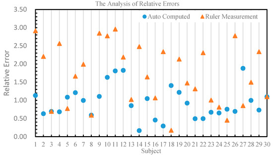
Figure 16.
The relative errors of the values calculated by our model and those measured by a ruler as compared to the values measured by an auto-refractometer.
Husna et al. [39] investigated the feasibility of using a smartphone to measure the distance between pupils and compared the measurement results of different applications with those of a standard automatic refractometer. The study found that the measurement results of the GlassifyMe application were not significantly different from those of the standard automatic refractometer, indicating that this application could be used as an alternative method for measuring the distance between pupils. This finding is consistent with the present study, and thus the model proposed in this paper can serve as a foundation for developing health measurement devices.
In conclusion, after conducting a comprehensive analysis of the experimental results, our proposed method exhibits numerous advantages compared to traditional ruler-based measurements and an auto-refractometer method. These advantages include high accuracy, simplicity of operation, non-contact measurement, affordability, and short measurement time. A comprehensive comparison in Table 4 provides detailed insights into various aspects of comparison.
Table 4.
Comparison of the advantages and disadvantages of three methods.
5. Conclusions
This paper aims to investigate the measurement of pupillary distance and height and proposes a measurement scheme based on an integrated regression tree and BlendMask algorithm. In our proposed method, we first utilize an open dataset to create labels and train a facial keypoint detection model. After obtaining the coordinates of the key points in the eye region, we calculate the position information of the pupils. Next, we create a dataset for glasses recognition, train a BlendMask detection model, identify the glasses lens, and obtain the lowest point information of the lens. Finally, we calculate the pupillary distance and height using the pupil coordinates and the lowest point coordinates of the lens. The experimental results demonstrate that our proposed method accurately calculates pupillary distance and height and is suitable for various scenarios. Using the values measured by an auto-refractometer as a standard, the relative error of pupillary distance calculated by our model in this paper is below 2%, and the accuracy is higher than that of measuring with a ruler. The results are highly consistent with the measurements obtained by an auto-refractometer. Furthermore, we have deployed the program on mobile devices, making it convenient to measure pupillary distance and height anytime and anywhere. Although this framework can be deployed on various platforms, the program is relatively complex, and certain human factors can affect the measurement results, such as the face not being parallel to the camera or the head having a deflection angle when taking photos, which can cause data deviation. Therefore, in the future, we will focus on simplifying the program framework and optimizing the program to eliminate interference from human factors.
Author Contributions
Conceptualization, H.X.; Methodology, Z.Z. and H.X.; Software, Z.Z. and D.L.; Validation, D.L.; Investigation, Z.Z. and D.L.; Resources, C.L.; Writing—original draft, Z.Z.; Writing—review & editing, H.X. and C.L.; Supervision, C.L. All authors have read and agreed to the published version of the manuscript.
Funding
Postgraduate Scientific Research Capability Enhancement Program Project Funding 2023.
Institutional Review Board Statement
Not applicable.
Informed Consent Statement
Not applicable.
Data Availability Statement
Our image dataset mainly comes from the 300W dataset and the CAS-PEAL-R1 dataset.
Conflicts of Interest
The authors declare no conflict of interest.
References
- Boraston, Z.; Blakemore, S.J. The application of eye-tracking technology in the study of autism. J. Physiol. 2007, 581, 893–898. [Google Scholar] [CrossRef] [PubMed]
- Kasprowski, P.; Dzierzega, M.; Kruk, K.; Harezlak, K.; Filipek, E. Application of eye tracking to support children’s vision enhancing exercises. In Advances in Intelligent Systems and Computing, Proceedings of the Information Technologies in Medicine: 5th International Conference, ITIB 2016, Kamień Śląski, Poland, 20–22 June 2016 Proceedings, Volume 1; Springer International Publishing: Cham, Switzerland, 2016; pp. 75–84. [Google Scholar]
- Raudonis, V.; Simutis, R.; Narvydas, G. Discrete eye tracking for medical applications. In Proceedings of the 2009 2nd International Symposium on Applied Sciences in Biomedical and Communication Technologies, Bratislava, Slovakia, 24–27 November 2009; pp. 1–6. [Google Scholar]
- Chen, Y.; Tsai, M.J. Eye-hand coordination strategies during active video game playing: An eye-tracking study. Comput. Hum. Behav. 2015, 51, 8–14. [Google Scholar] [CrossRef]
- Chandra, S.; Sharma, G.; Malhotra, S.; Jha, D.; Mittal, A.P. Eye tracking based human computer interaction: Applications and their uses. In Proceedings of the 2015 International Conference on Man and Machine Interfacing (MAMI), Bhubaneswar, India, 17–19 December 2015; pp. 1–5. [Google Scholar]
- Giancoli, D.C.; Miller, I.A.; Puri, O.P.; Zober, P.J.; Zober, G.P. Physics: Principles with Applications; Pearson/Prentice Hall: Upper Saddle River, NJ, USA, 1998. [Google Scholar]
- Yildirim, Y.; Sahbaz, I.; Kar, T.; Kagan, G.; Taner, M.T.; Armagan, I.; Cakici, B. Evaluation of interpupillary distance in the Turkish population. Clin. Ophthalmol. 2015, 9, 1413–1416. [Google Scholar] [CrossRef] [PubMed]
- Min-Allah, N.; Jan, F.; Alrashed, S. Pupil detection schemes in human eye: A review. Multimed. Syst. 2021, 27, 753–777. [Google Scholar] [CrossRef]
- Qiu, Y.; Xu, X.; Qiu, L.; Pan, Y.; Wu, Y.; Chen, W.; Han, X. 3dcaricshop: A dataset and a baseline method for single-view 3d caricature face reconstruction. In Proceedings of the IEEE/CVF Conference on Computer Vision and Pattern Recognition, Nashville, TN, USA, 20–25 June 2021; pp. 10236–10245. [Google Scholar]
- Wu, J.; Zhou, Z. Efficient face candidates selector for face detection. Pattern Recognit. 2003, 36, 1175–1186. [Google Scholar] [CrossRef]
- Ban, Y.; Kim, S.-K.; Kim, S.; Toh, K.-A.; Lee, S. Face detection based on skin color likelihood. Pattern Recognit. 2014, 47, 1573–1585. [Google Scholar] [CrossRef]
- Karaaba, M.F.; Schomaker, L.; Wiering, M. Machine learning for multi-view eyepair detection. Eng. Appl. Artif. Intell. 2014, 33, 69–79. [Google Scholar] [CrossRef]
- Long, L. Research on Face Detection and Eye Location Algorithm Based on Adaboost; University of Electronic Science and Technology: Chengdu, China, 2008. (In Chinese) [Google Scholar]
- Lin, M. Research on Face Recognition Based on Deep Learning; Dalian University of Technology: Dalian, China, 2013. (In Chinese) [Google Scholar]
- Wang, C.; Chang, L. A precise eye localization method based on region projection. J. Optoelectron. Laser 2011, 4, 618–622. [Google Scholar]
- Kumar, R.T.; Raja, S.K.; Ramakrishnan, A.G. Eye detection using color cues and projection functions. In Proceedings of the 2002 International Conference on International Conference on Image Processing, Rochester, NY, USA, 22–25 September 2002; Volume 3, pp. 337–340. [Google Scholar]
- Wu, Y.; Yang, Y.; Wang, L.P. An Eye Location Algorithm Based on the Gray Information and the Pupil Filter. Comput. Eng. Appl. 2005, 41, 45–47. [Google Scholar]
- Xu, G.F.; Huang, L.; Liu, C.P.; Ding, S.Q. Eye Location Using Hierarchical Classifier. J. Chin. Comput. Syst. 2008, 29, 1158–1162. [Google Scholar]
- Kazemi, V.; Sullivan, J. One millisecond face alignment with an ensemble of regression trees. In Proceedings of the IEEE Conference on Computer Vision and Pattern Recognition, Columbus, OH, USA, 23–28 June 2014; pp. 1867–1874. [Google Scholar]
- LeCun, Y.; Bengio, Y.; Hinton, G. Deep learning. Nature 2015, 521, 436–444. [Google Scholar] [CrossRef] [PubMed]
- Krizhevsky, A.; Sutskever, I.; Hinton, G.E. Imagenet classification with deep convolutional neural networks. Commun. ACM 2017, 60, 84–90. [Google Scholar]
- Zeiler, M.D.; Fergus, R. Visualizing and understanding convolutional networks. In Lecture Notes in Computer Science, Proceedings of the Computer Vision–ECCV 2014: 13th European Conference, Zurich, Switzerland, 6–12 September 2014, Proceedings, Part I 13; Springer International Publishing: Cham, Switzerland, 2014; pp. 818–833. [Google Scholar]
- He, K.; Gkioxari, G.; Dollár, P.; Girshick, R. Mask r-cnn. In Proceedings of the IEEE International Conference on Computer Vision, Venice, Italy, 22–29 October 2017; pp. 2961–2969. [Google Scholar]
- Girshick, R. Fast r-cnn. In Proceedings of the IEEE International Conference on Computer Vision, Santiago, Chile, 7–13 December 2015; pp. 1440–1448. [Google Scholar]
- Ren, S.; He, K.; Girshick, R.; Sun, J. Faster R-CNN: Towards Real-Time Object Detection with Region Proposal Networks. IEEE Trans. Pattern Anal. Mach. Intell. 2017, 39, 1137–1149. [Google Scholar] [CrossRef] [PubMed]
- Lin, T.Y.; Dollár, P.; Girshick, R.; He, K.; Hariharan, B.; Belongie, S. Feature pyramid networks for object detection. In Proceedings of the IEEE conference on Computer Vision and Pattern Recognition, Honolulu, HI, USA, 21–26 July 2017; pp. 2117–2125. [Google Scholar]
- Lin, T.Y.; Maire, M.; Belongie, S.; Hays, J.; Perona, P.; Ramanan, D.; Dollár, P.; Zitnick, C.L. Microsoft coco: Common objects in context. In Lecture Notes in Computer Science, Proceedings of the Computer Vision–ECCV 2014: 13th European Conference, Zurich, Switzerland, 6–12 September 2014, Proceedings, Part V 13; Springer International Publishing: Cham, Switzerland, 2014; pp. 740–755. [Google Scholar]
- Cordts, M.; Omran, M.; Ramos, S.; Rehfeld, T.; Enzweiler, M.; Benenson, R.; Franke, U.; Roth, S.; Schiele, B. The cityscapes dataset for semantic urban scene understanding. In Proceedings of the IEEE Conference on Computer Vision and Pattern Recognition, Las Vegas, NV, USA, 27–30 June 2016; pp. 3213–3223. [Google Scholar]
- Neuhold, G.; Ollmann, T.; Rota Bulo, S.; Kontschieder, P. The mapillary vistas dataset for semantic understanding of street scenes. In Proceedings of the IEEE International Conference on Computer Vision, Venice, Italy, 22–29 October 2017; pp. 4990–4999. [Google Scholar]
- Hafiz, A.M.; Bhat, G.M. A survey on instance segmentation: State of the art. Int. J. Multimed. Inf. Retr. 2020, 9, 171–189. [Google Scholar] [CrossRef]
- Chen, H.; Sun, K.; Tian, Z.; Shen, C.; Huang, Y.; Yan, Y. Blendmask: Top-down meets bottom-up for instance segmentation. In Proceedings of the IEEE/CVF Conference on Computer Vision and Pattern Recognition, Seattle, WA, USA, 13–19 June 2020; pp. 8573–8581. [Google Scholar]
- Sagonas, C.; Tzimiropoulos, G.; Zafeiriou, S.; Pantic, M. 300 faces in-the-wild challenge: The first facial landmark localization challenge. In Proceedings of the IEEE International Conference on Computer Vision Workshops, Sydney, Australia, 2–8 December 2013; pp. 397–403. [Google Scholar]
- Tian, Z.; Shen, C.; Chen, H.; He, T. Fcos: Fully convolutional one-stage object detection. In Proceedings of the IEEE/CVF International Conference on Computer Vision, Seoul, Republic of Korea, 27 October–2 November 2019; pp. 9627–9636. [Google Scholar]
- Li, Y.; Qi, H.; Dai, J.; Ji, X.; Wei, Y. Fully convolutional instance-aware semantic segmentation. In Proceedings of the IEEE Conference on Computer Vision and Pattern Recognition, Honolulu, HI, USA, 21–26 July 2017; pp. 2359–2367. [Google Scholar]
- Bolya, D.; Zhou, C.; Xiao, F.; Lee, Y.J. Yolact: Real-time instance segmentation. In Proceedings of the IEEE/CVF International Conference on Computer Vision, Seoul, Republic of Korea, 27 October–2 November 2019; pp. 9157–9166. [Google Scholar]
- Chen, L.C.; Zhu, Y.; Papandreou, G.; Schroff, F.; Adam, H. Encoder-decoder with atrous separable convolution for semantic image segmentation. In Proceedings of the European Conference on Computer Vision (ECCV), Munich, Germany, 8–14 September 2018; pp. 801–818. [Google Scholar]
- Mallick, S. Head pose estimation using OpenCV and Dlib. Learn OpenCV 2016, 1–26. [Google Scholar]
- Zhang, E.; Zhang, Y. Average Precision. In Encyclopedia of Database Systems; Liu, L., Özsu, M.T., Eds.; Springer: Boston, MA, USA, 2009. [Google Scholar] [CrossRef]
- Husna, H.N.; Fitriani, N. Evaluation of Pupillary Distance (PD) Measurement using Smartphone-based Pupilometer. J. Phys. Conf. Ser. 2022, 2243, 012001. [Google Scholar] [CrossRef]


Disclaimer/Publisher’s Note: The statements, opinions and data contained in all publications are solely those of the individual author(s) and contributor(s) and not of MDPI and/or the editor(s). MDPI and/or the editor(s) disclaim responsibility for any injury to people or property resulting from any ideas, methods, instructions or products referred to in the content. |
© 2023 by the authors. Licensee MDPI, Basel, Switzerland. This article is an open access article distributed under the terms and conditions of the Creative Commons Attribution (CC BY) license (https://creativecommons.org/licenses/by/4.0/).