Evaluating the Effect of Road Surface Potholes Using a Microscopic Traffic Model

Abstract

Road surface wear leads to the formation of cracks and holes known as potholes. Potholes disrupt the smooth flow of traffic and can lead to accidents. The Intelligent Driver (ID) model is commonly employed but it assumes uniform traffic behavior for all conditions. This oversimplified approach is unrealistic as it does not consider the impact of real-world factors such as potholes on traffic patterns. This paper proposes a microscopic traffic model to address the impact of these road surface irregularities on traffic. The effect of small, medium, and large conical potholes is investigated using fundamental diagrams for traffic flow and velocity. The results obtained indicate that the proposed model outperforms the ID model as it can more accurately characterize how potholes and driver sensitivity affect vehicle behavior.

1. Introduction

Road surfaces develop cracks and holes over time which lead to the formation of potholes [1]. Potholes are an important factor in road networks, particularly in developing countries. They affect the smooth flow of traffic and cause discomfort and steering misalignment [2]. Potholes are formed when water penetrates cracks in the road surface commonly caused by wear. This is exacerbated by extreme weather conditions, heavy traffic, and poor drainage [1]. Potholes cause traffic delays and accidents [3]. Thus, it is important to consider the impact of potholes on traffic flow.

Potholes cause loss of control and lead to accidents. In $2021$, potholes accounted for $0.8\mathrm{\%}$ of road accidents resulting in $1.4\mathrm{\%}$ of fatalities and $0.6\mathrm{\%}$ of injuries [4]. Road surface irregularities have been shown to reduce vehicle speeds by $55\mathrm{\%}$ and increase emissions by $2.49\mathrm{\%}$ [5]. The Canadian Automobile Association (CAA) reported that potholes increase operating costs by 3 billion dollars annually [6]. In addition, poor road conditions lead to congestion and driver frustration which can result in dangerous driving behavior [7]. Realistic traffic flow models are needed to alleviate these problems.

Traffic models can be categorized as microscopic, macroscopic, or mesoscopic. Microscopic models consider individual vehicle behavior and employ parameters such as position, velocity, and time and distance headways [8,9]. They often incorporate driver psychological and physical responses [10] and are used to predict vehicle dynamics [11].

The first microscopic models were developed by Pipes [12] and Reuschel [13] but cannot accurately characterize traffic flow. Later, Newell [14] created a model based on driver behavior in congested traffic. In this model, a larger distance headway results in higher velocity, and this headway is small during congestion. However, it can produce excessive acceleration which is not realistic [15]. Bando et al. [16] developed a model according to the equilibrium velocity distribution based on density. With this model, a decrease in velocity results in a larger density. However, deviations from this distribution lead to uniform acceleration, which is unrealistic. In addition, traffic behavior can be unstable because velocity differences are not taken into account [17]. Helbing and Tilch [18] proposed a model which employs velocity differences. However, it only considers aggressive driver behavior as acceleration occurs over a short time. Gipps [19] characterized traffic based on driver response but the resulting model is only accurate for a small range of parameters [11].

Treiber et al. [15] developed a car following model commonly known as the intelligent driver (ID) model. It can better characterize traffic than previous models [20,21,22] as it incorporates practical traffic parameters [11]. Driver behavior is based on the distance headway and velocity of leading vehicles [23,24,25]. However, an acceleration exponent is employed which does not capture traffic dynamics, leading to unrealistic behavior. The ID model was improved by incorporating driver reaction to leading vehicles [26], driver safety [27], and the velocity at intersections [28]. However, the velocity can be high when the distance between vehicles is small which can result in accidents.

The PTV Vissum model [29] uses field data from eight intersections. Simulated and observed conflicts were employed to determine suitable thresholds for the time to collision. The relationship between simulated and observed conflicts was confirmed in [29]. The accuracy of the PTV Vissum model and Surrogate Safety Assessment Model (SSAM) in estimating pedestrian–vehicle conflicts at signalized intersections was examined in [30]. In addition, partial Crossover Displaced Left-turn intersection (XDL) versus full XDL designs were considered in [31] to optimize intersection control. This resulted in improved capacity, reduced delays, and smaller queues. In [32], Median U-turn (MUT) intersections were shown to improve the operation and safety of vehicles, pedestrians, and cyclists. In [33], route diversion through congestion pricing strategies using a microscopic traffic model was shown to reduce travel time by 10–16%. Carbon dioxide (CO₂) emissions were predicted in [34] using a microscopic transportation emission model. The results obtained can help in developing environmental transportation policies.

The influence of road surface conditions on traffic is a crucial factor in traffic modeling. In [35], a model was proposed to examine the impact of road surface conditions on traffic flow. The results obtained reveal that a well-maintained road surface improves both traffic flow and speed [1]. However, this model does not characterize the quantitative effect of road surface conditions, in particular, the combined effect [35]. Explicit expressions were given in [36] to characterize the effect of road surface conditions on traffic flow. In addition, a macroscopic traffic model was developed in [1] which considers potholes. Similar models have been developed which consider road surface conditions but to date, there are no microscopic traffic models.

In this paper, a new microscopic traffic model is presented which characterizes the effect of potholes on traffic behavior. The ID model does not consider road surface conditions and employs a constant acceleration exponent, so it can result in unrealistic traffic behavior. The performance of the proposed and ID models is evaluated on a single-lane circular road of length $1$ km. A platoon of $31$ vehicles is considered for $200$ s. The results obtained indicate that the proposed model accurately captures the impact of real-world factors such as potholes on traffic.

The remainder of this paper is organized as follows. Section 2 presents the model formulation. The performance is evaluated in Section 3 and Section 4 provide some concluding remarks.

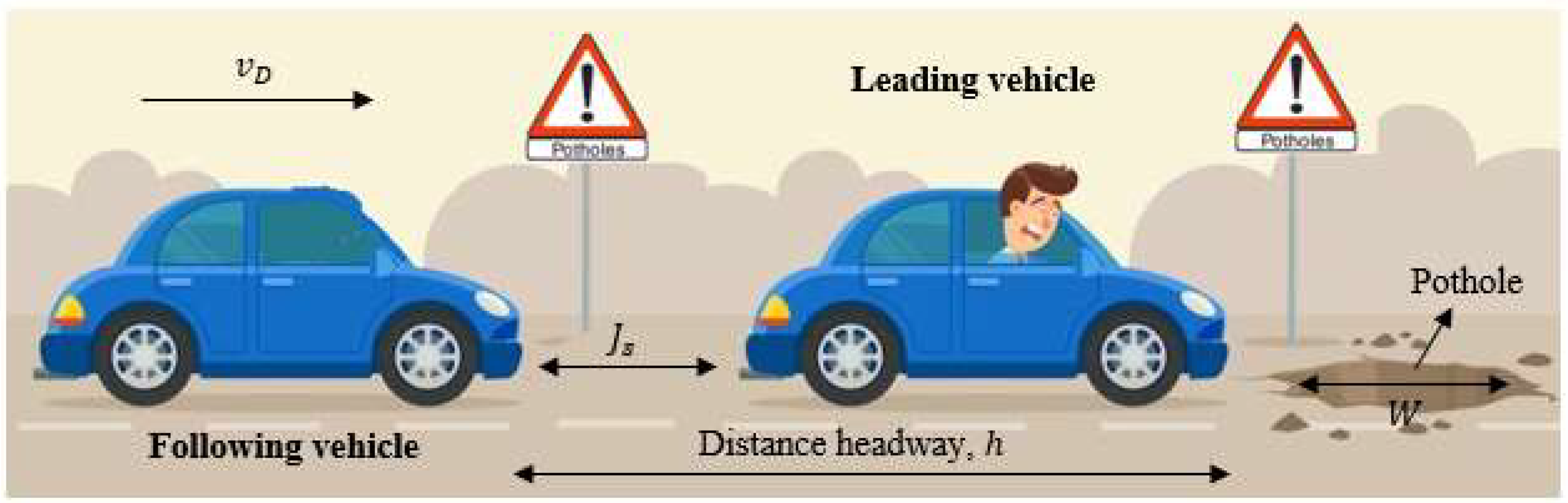
2. Model Formulation

The Intelligent Driver (ID) model is a microscopic traffic model which uses a second-order differential equation to characterize vehicle dynamics in congested and free-flow conditions [23]. It considers forward vehicles and the driver response according to the relative velocity [25]. The driver response is determined by the ratio of average velocity to desired velocity. When this ratio is equal to 1, the flow is smooth, and acceleration and deceleration are small [37]. According to the ID model, acceleration is influenced by driver response, the ratio of desired distance headway to distance headway, and the velocity difference between vehicles. Acceleration with this model is given by [15]

$$\dot{v}=a_{max}\left(1-{\left(\frac{v}{v_{\mathrm{D}}}\right)}^{\delta }-{\left(\frac{s^{*}}{h}\right)}^2\right)$$

(1)

where $a_{max}$ is the maximum acceleration; $v$ and $v_D$ are the average velocity and desired velocity, respectively; $h$ is the distance headway; and $\delta$ is the acceleration exponent. The desired distance headway, denoted as $s^{*}$, is given by [15]

$$s^{*}=J_s+Tv+\frac{v∆v}{2\sqrt{a_{max}b}}$$

(2)

where $J_s$ is the distance between vehicles during congestion, called the jam spacing, as shown in Figure 1; $T$ is the time headway; $∆v$ is the velocity difference between vehicles; and $b$ is the deceleration (minimum acceleration). The ID model employs (1) and (2) to characterize traffic behavior.

The acceleration exponent $\delta$ in the ID model is a constant which can result in unrealistic traffic characterization as it is not based on traffic physics. Traffic behavior is affected by the environment, including road surface conditions. Therefore, a variable exponent is proposed to realistically characterize traffic flow based on potholes. The road surface irregularity can be expressed as [1,38,39]

$$-\frac{D}{2}\left(1-\mathrm{c}\mathrm{o}\mathrm{s}\frac{2\pi \theta }{W}\right)$$

(3)

where $D$ and $W$ are the depth and width of the pothole, respectively; θ represents a location within the pothole measured from the farthest point on the left; and $D<0$ denotes a bulging road surface whereas $D=0$ denotes a smooth road surface without any holes or cracks. It is presumed that potholes have a conical shape but with a smaller height. Thus, the size of a pothole can be approximated as [1]

$$P_s=-\frac{1}{2}\pi W\sqrt{\frac{W^2}{4}+D^2}$$

(4)

The impact of potholes on the traffic flow primarily depends on the distance headway. For a large distance headway, the distance between vehicles is large so drivers have more time to react to road surface irregularities. Thus, they can maneuver around potholes. Conversely, if the distance headway is small, the impact of these irregularities is more significant as drivers have less time to react. Thus, (4) can be rewritten as

$$P_s=-\frac{1}{2}\pi W\left(\frac{\tau }{{\tau }_N}\right)\left(1-\frac{h}{h_s}\right)\sqrt{\frac{W^2}{4}+D^2}$$

(5)

where $\tau$ is the reaction time of a driver; ${\tau }_N$ is the typical reaction time; and $h_s$ is the safe distance headway. Driver sensitivity is defined as $\frac{\tau }{{\tau }_N}$. A driver is aggressive when $\tau <{\tau }_N$, sluggish when $\tau >{\tau }_N$, and typical when $\tau ={\tau }_N$. Aggressive drivers have a short reaction time and often maintain their speed when potholes are present [1]. In contrast, sluggish drivers have a large reaction time and tend to slow when potholes are present regardless of their size. Substituting (5) for $\delta$ in (1) gives the acceleration for the proposed model as

$$\dot{v}=a_{max}\left(1-{\left(\frac{v}{v_{\mathrm{D}}}\right)}^{-\frac{1}{2}\pi W\left(\frac{\tau }{{\tau }_N}\right)\left(1-\frac{h}{h_s}\right)\sqrt{\frac{W^2}{4}+D^2}}-{\left(\frac{s^{*}}{h}\right)}^2\right)$$

(6)

This characterizes traffic based on pothole size and driver sensitivity and so is more accurate and realistic than with a fixed $\delta$. Thus, the acceleration varies according to the environment, unlike the ID model which produces similar behavior for all road surface conditions.

Traffic flow is the ratio of velocity and distance headway at equilibrium and so can be expressed as [23,40]

$$f=\frac{v}{h_e}$$

(7)

At equilibrium, the velocity difference is equal to zero and thus the equilibrium distance headway for the proposed model is

$$h_e=\left(J_s+Tv\right){\left(1-{\left(\frac{v}{v_D}\right)}^{-\frac{1}{2}\pi W\left(\frac{\tau }{{\tau }_N}\right)\left(1-\frac{h}{h_s}\right)\sqrt{\frac{W^2}{4}+D^2}}\right)}^{-1/2}$$

(8)

Substituting (8) in (7) gives the flow for the proposed model as

$$f=\frac{v}{\left(J_s+Tv\right){\left(1-{\left(\frac{v}{v_D}\right)}^{-\frac{1}{2}\pi W\left(\frac{\tau }{{\tau }_N}\right)\left(1-\frac{h}{h_s}\right)\sqrt{\frac{W^2}{4}+D^2}}\right)}^{-1/2}}$$

(9)

Thus, traffic flow varies based on the road surface conditions and driver sensitivity. With a high sensitivity, driver reaction is fast and hence the flow is large as traffic conditions are predictable. Conversely, less sensitive drivers react more slowly to changes in the environment so the flow is large and congestion may occur. Furthermore, large-size potholes result in larger changes in traffic flow.

3. Performance Evaluation

In this section, the performance of the ID and proposed models is evaluated over a $1$ km circular road for $200$ s with a platoon of $31$ vehicles. The explicit Euler technique with time step $0.5$ s is used to implement both models. The simulation parameters are given in

Table 1. Simulation parameters.

Parameter	Value
Desired velocity, $v_D$	$33.3$ m/s
Time headway for the ID and proposed model, $T$	$1$ .0 s
Proposed model distance headway, $h$	$21.0$ m
Safe distance headway, $h_s$	$5.0$ m
Reaction time of an aggressive driver, $\tau$	$0.5$ s
Reaction time of a sluggish driver, $\tau$	$6.0$ s
Reaction time of a typical driver, $\tau$	$3.0$ s
Typical driver reaction time, ${\tau }_N$	$3.0$ s
Jam spacing, $J_s$	$2.0$ m
Maximum acceleration, $a_{max}$	$0.73$ m/s2
Minimum acceleration or deceleration, $b$	$1.67$ m/s2
Vehicle length, $L$	$5.0$ m
Acceleration exponent, $\delta$	$1.0, 4.0,$ and $200$
Time step, $∆t$	$0.5$ s
Maximum normalized density, $d_m=\frac{1}{J_s}$	$0.5$

.

It is important to select realistic model parameters. Therefore, the parameters considered are the same as in [41]. For the proposed model, $\tau =0.5$ s means $\frac{\tau }{{\tau }_N}<1$ indicating an aggressive driver, $\tau =6.0$ s means $\frac{\tau }{{\tau }_N}>1$ indicating a sluggish driver, and $\tau =3.0$ s means $\frac{\tau }{{\tau }_N}=1$ indicating a typical driver [1]. The distance headway is $h=21.0$ m [11], the safe distance headway is $h_s=5.0$ m [42], and the time headway for both models is $T=1.0$ s [43]. The value of $\delta$ ranges between $1.0$ and $\infty$ and is typically $4.0$ [15], hence the ID model is evaluated for $\delta =1.0, 4.0,$ and $200$. The maximum normalized density is $d_m=0.5$.

In terms of size, potholes can be categorized as small, medium, or large with widths between $0.5$ and $3.5$ m and depths between $0$ and $0.3$ m [1]. Potholes with a width less than or equal to $0.70$ m are classified as small, with a width greater than $1.7$ m as large, and in between as medium. The pothole dimensions considered are given in

Table 2. Pothole sizes and the corresponding dimensions.

Pothole Size	Width, W (m)	Depth, D (m)
Small	$0.7$	$0.1$
Medium	$1.7$	$0.2$
Large	$3.0$	$0.3$

.

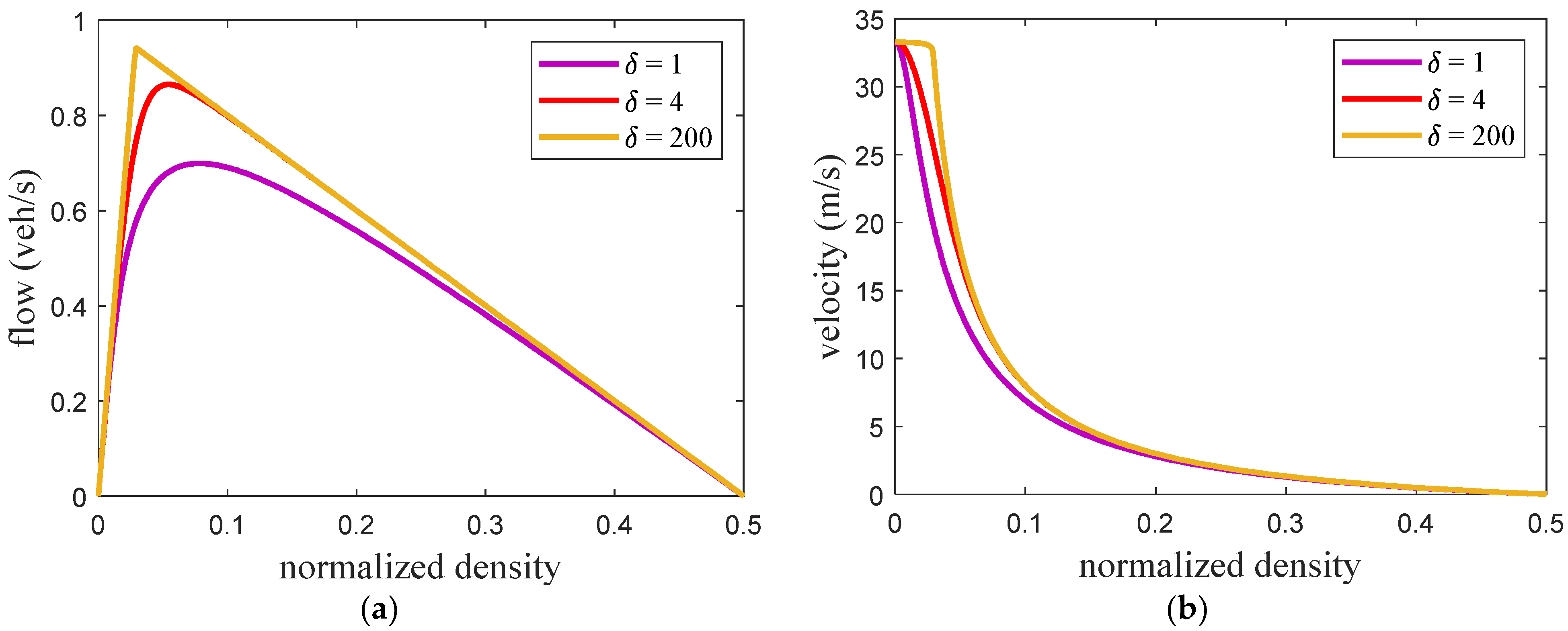
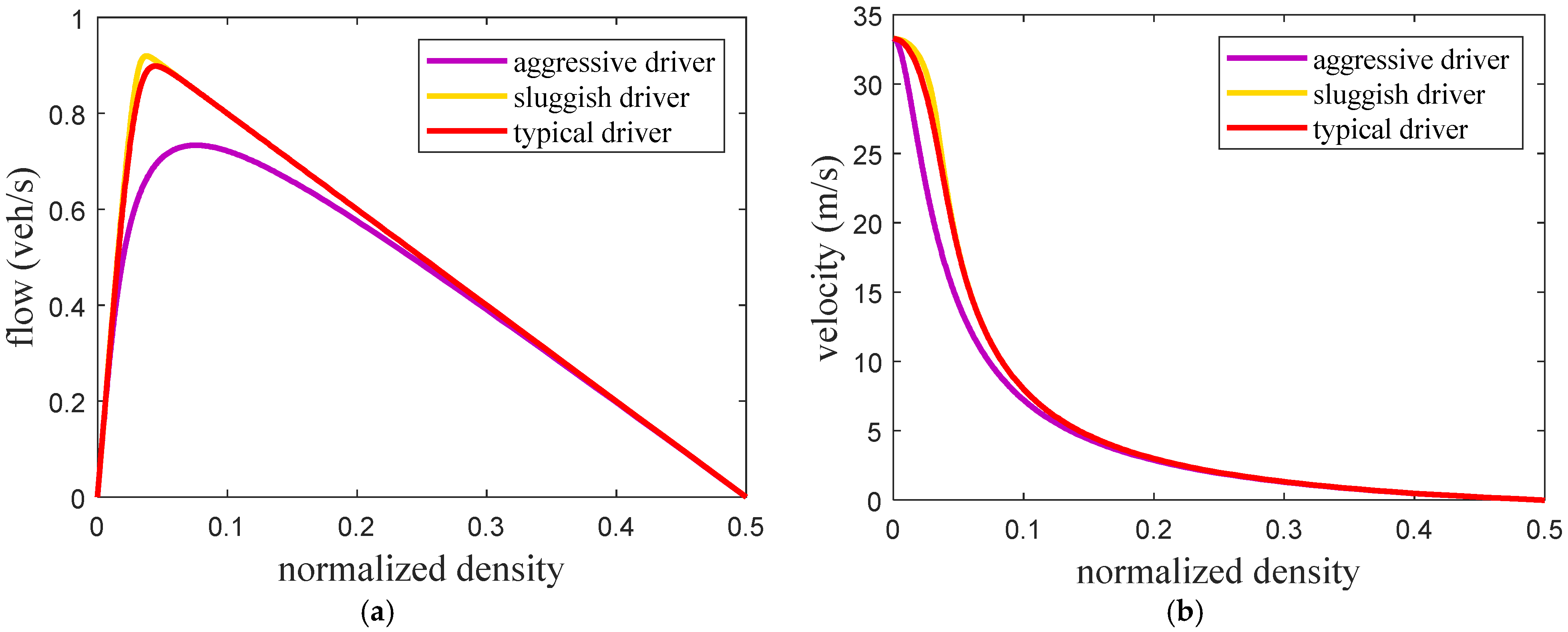
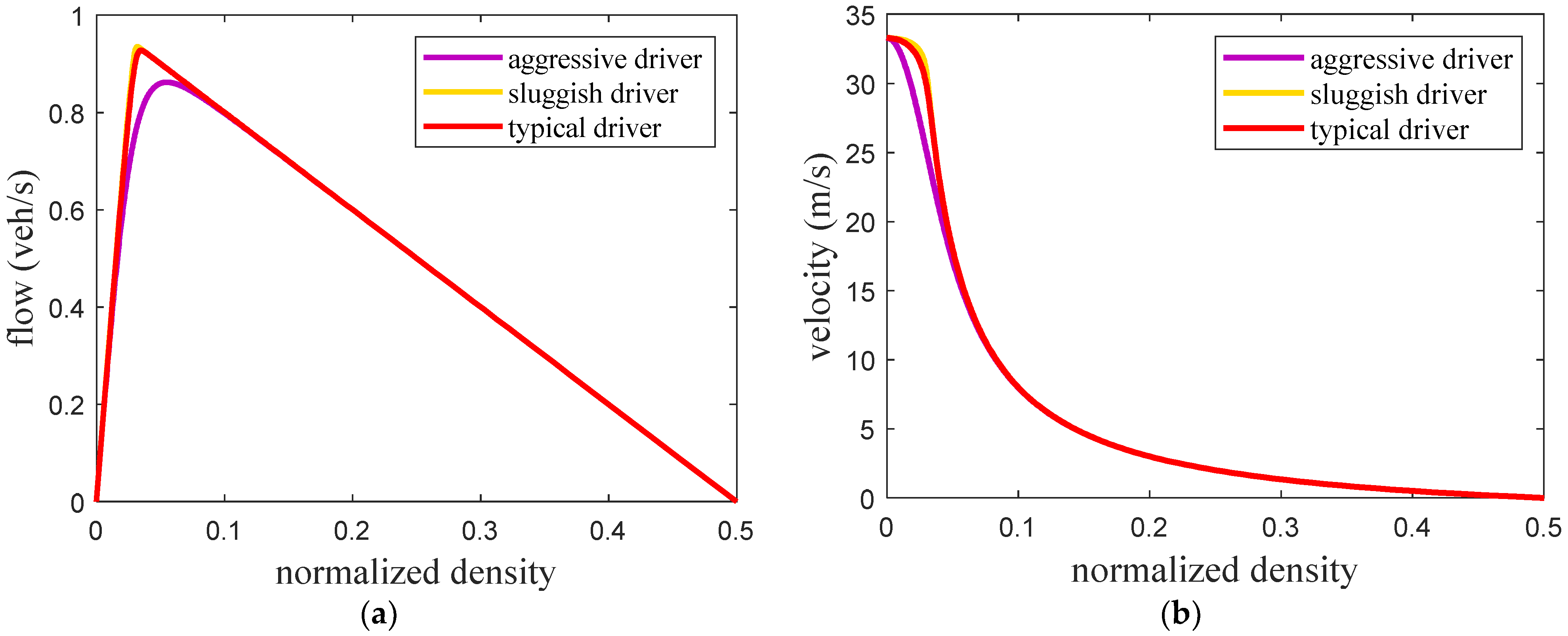
3.1. Fundamental Diagrams

Figure 2 presents the fundamental diagrams for the ID model with $\delta =1.0, 4.0,$ and $200$. This shows that a larger $\delta$ results in a greater traffic flow. The maximum flow, critical density at maximum flow, and critical velocity are given in

Table 3. Maximum flow, critical density, and velocity for the ID model.

$\mathbf{Acceleration} \mathbf{Exponent} \left(\mathit{\delta }\right)$	Maximum Flow (veh/s)	Critical Density	Critical Velocity (m/s)
$1.0$	$0.69$	$0.076$	$9.1$
$4.0$	$0.86$	$0.050$	$17.1$
$200$	$0.94$	$0.029$	$32.4$

. These results indicate that an increase in $\delta$ decreases the critical density at maximum flow but the corresponding velocity increases. Figure 3, Figure 4 and Figure 5 present the fundamental diagrams for the proposed model with small, medium, and large potholes, respectively.

Table 4. Maximum flow, critical density, and velocity for the proposed model with small, medium, and large potholes.

Pothole Size	Driver Sensitivity	Maximum Flow (veh/s)	Critical Density	Critical Velocity (m/s)
Small	Aggressive	$0.41$	$0.068$	$6.2$
	Sluggish	$0.82$	$0.064$	$12.8$
	Typical	$0.73$	$0.075$	$9.8$
Medium	Aggressive	$0.73$	$0.066$	$9.8$
	Sluggish	$0.91$	$0.036$	$24.9$
	Typical	$0.89$	$0.043$	$20.8$
Large	Aggressive	$0.86$	$0.055$	$15.5$
	Sluggish	$0.93$	$0.031$	$28.9$
	Typical	$0.92$	$0.034$	$26.9$

gives the maximum flow, critical velocity, and critical density at maximum flow for aggressive, sluggish, and typical drivers and small, medium, and large potholes. This shows that with small potholes, the road capacity is greater with a typical driver as the flow is larger when the density is high as shown in Figure 3a. Furthermore, for all driver types the maximum flow and critical velocity increase as the pothole size increases as shown in Table 4. In addition, an increase in the pothole size results in a greater change in maximum flow with an aggressive driver compared to sluggish and typical drivers. Thus, with the proposed model the relationship between flow, density, and velocity is based on road surface conditions and so is more realistic than with the ID model.

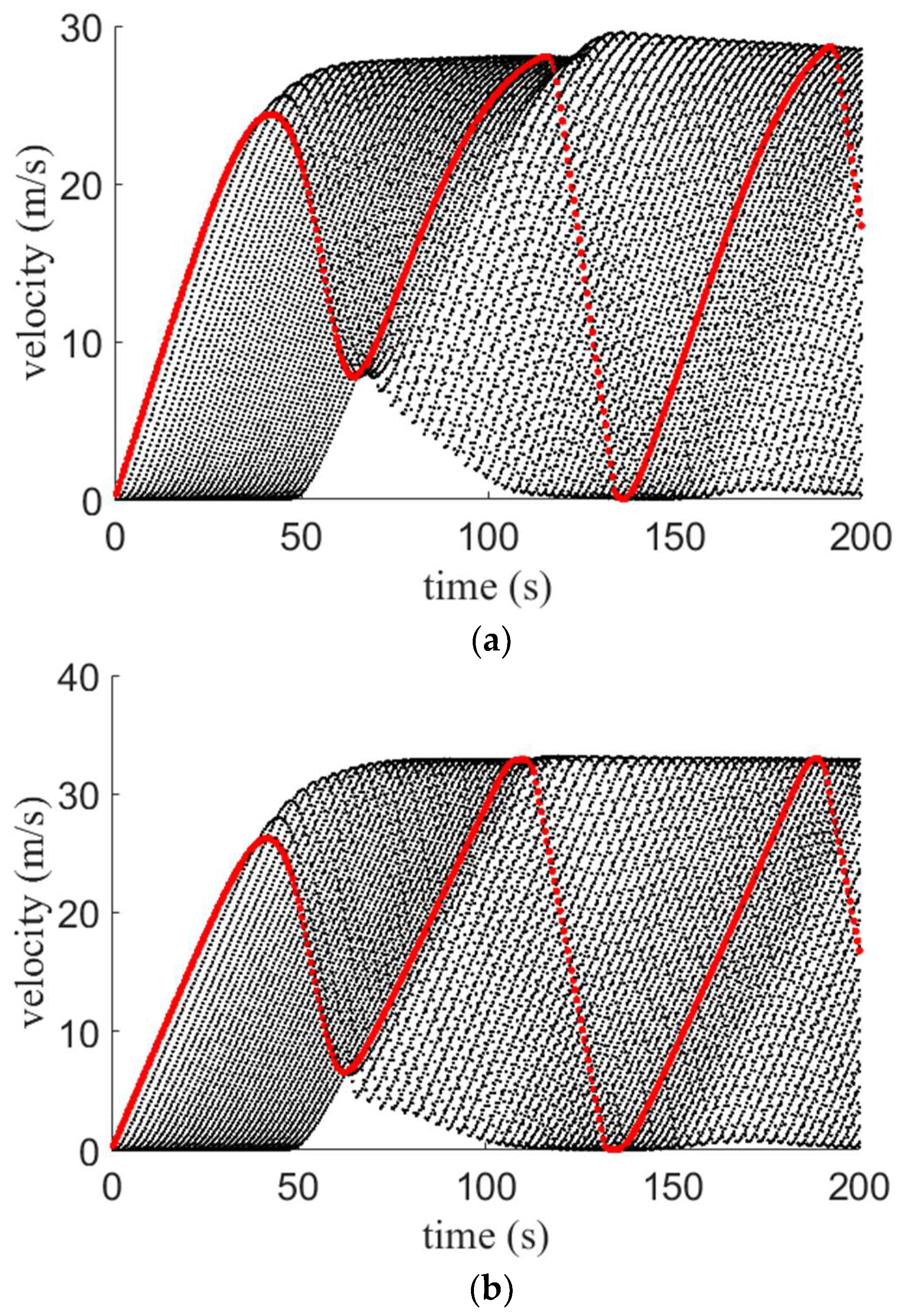
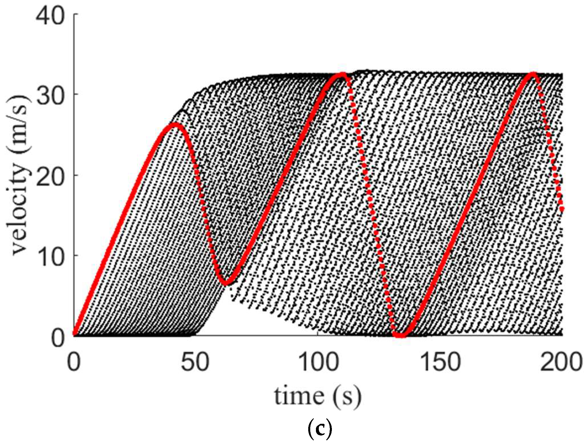
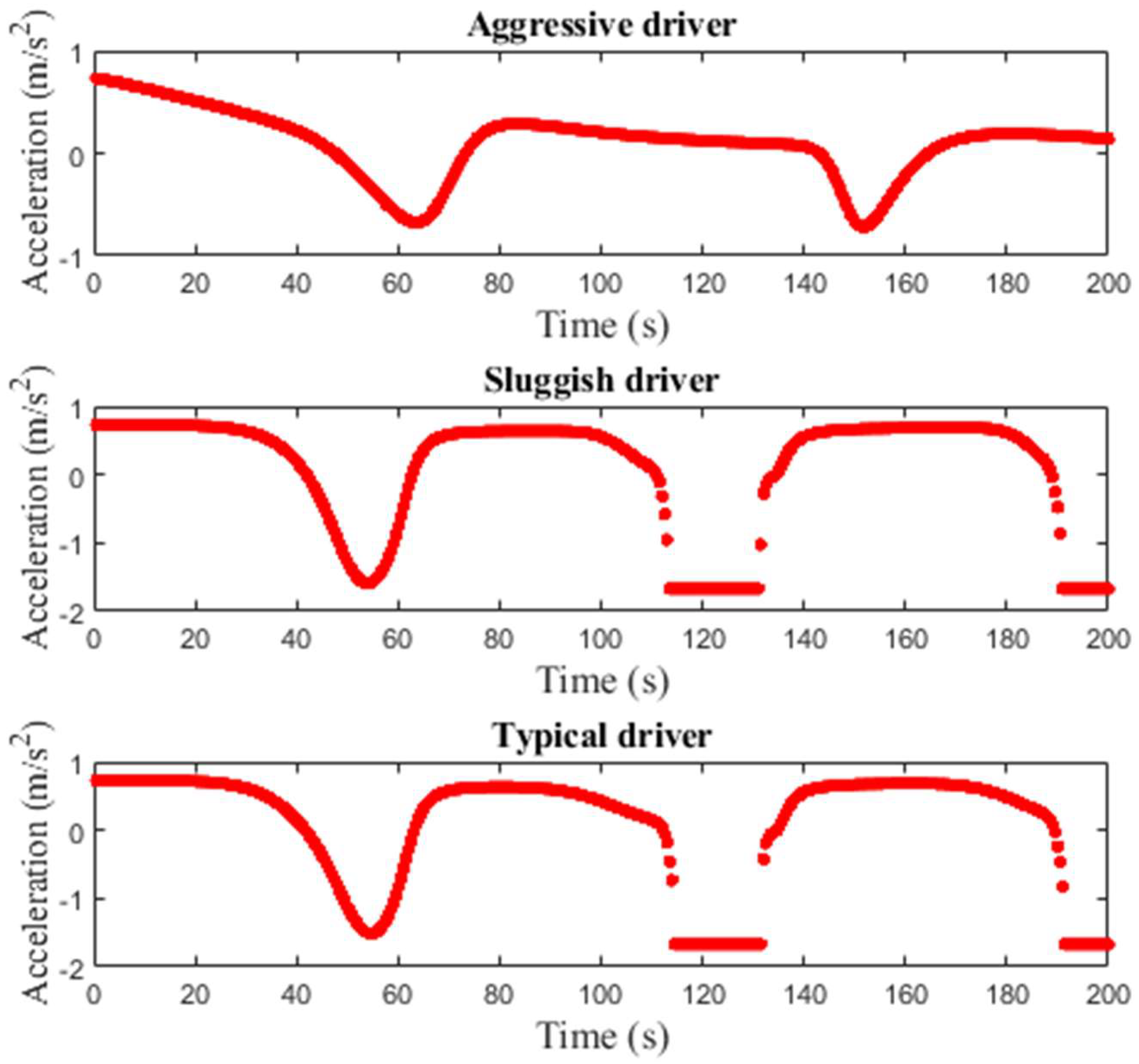
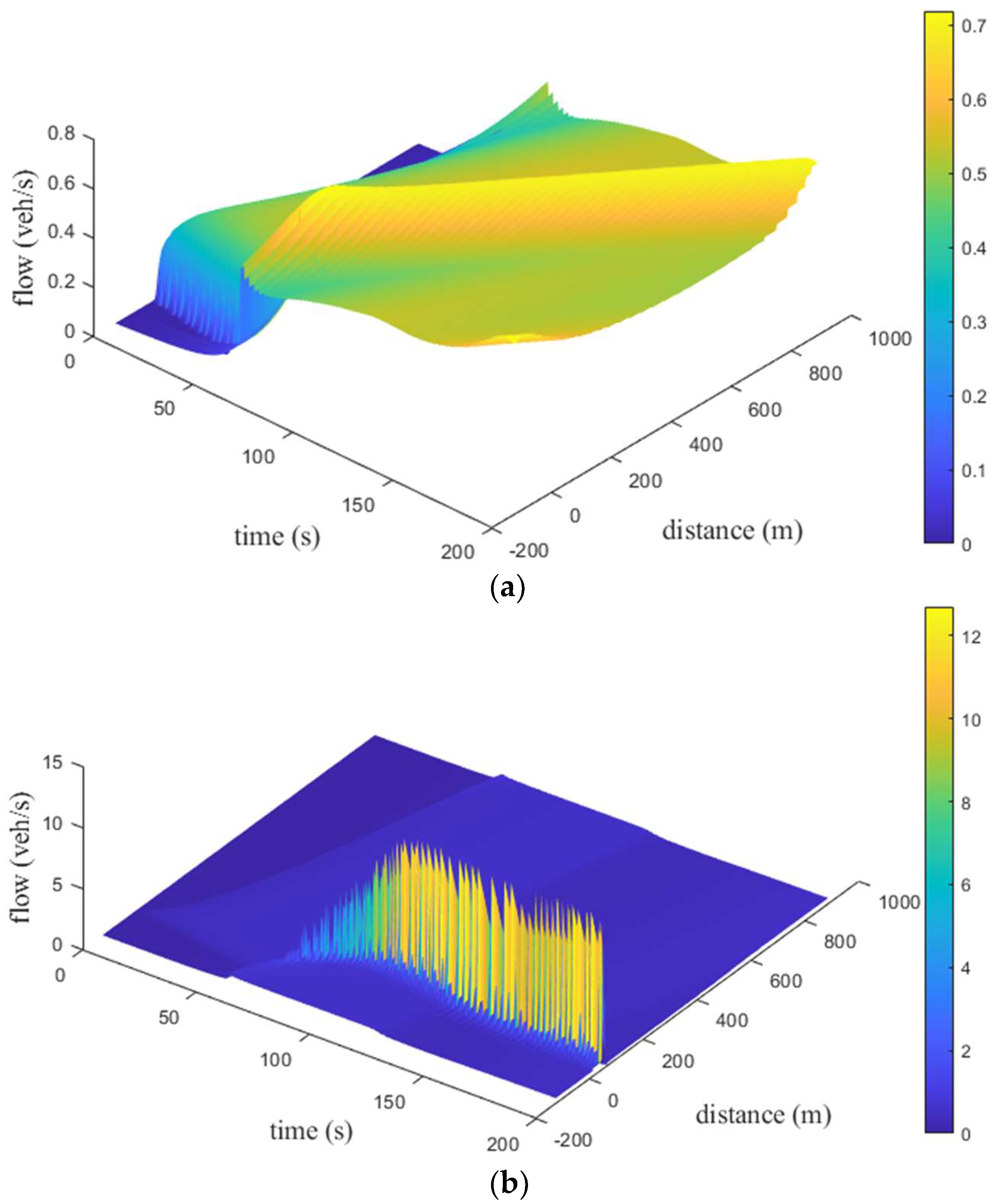
3.2. Performance Results

Figure 6 presents the velocity evolution over time for the ID model on a $1$ km circular road. The red line gives the velocity of the first vehicle and the black lines correspond to the velocity of the following vehicles. With $\delta =1.0$, the variations are small and decrease over time. The velocity is between $13.6$ and $21.6$ m/s at $200$ s as shown in Figure 6a. With $\delta =4.0$ and $200$, the variations in velocity are larger and increase over time as shown in Figure 6b,c. With $\delta =4.0$, the velocity is between $0.26$ and $28.6$ m/s at $200$ s, and with $\delta =200$ it is between $0.21$ and $33.1$ m/s at $200$ s. Thus, an increase in $\delta$ results in an increase in the variations in velocity.

Figure 7, Figure 8 and Figure 9 present the velocity evolution over time for the proposed model with small, medium, and large potholes, respectively. The red lines indicate the velocity of the first vehicle and the black lines correspond to the velocity of the following vehicles. For small potholes, with an aggressive driver, the variations over time are large and the velocity is between $0.74$ and $13.2$ m/s at $200$ s, as shown in Figure 7a. With a sluggish driver, the variations are small and decrease over time. The velocity is between $18.6$ and $25.6$ m/s at $200$ s, as shown in Figure 7b. With a typical driver, as expected the behavior is between that of aggressive and sluggish drivers with a velocity between $15.1$ and $22.9$ m/s at $200$ s, as shown in Figure 7c. For medium potholes, with an aggressive driver the variations in velocity over time are small and between $14.9$ and $22.6$ m/s at $200$ s, as shown in Figure 8a. With sluggish and typical drivers, the variations are large and increase over time, as shown in Figure 8b,c. With a sluggish driver, at $200$ s the velocity is between $0.20$ and $31.9$ m/s, and with a typical driver, it is between $0.28$ and $30.4$ m/s. For large potholes, the variations in velocity over time are large for all three types of drivers, as shown in Figure 9. With an aggressive driver, the velocity is between $0.38$ and $28.5$ m/s at $200$ s, as shown in Figure 9a. The corresponding velocity for a sluggish driver is between $0.26$ and $32.9$ m/s and for a typical driver is between $0.16$ and $32.4$ m/s as shown in Figure 9b,c, respectively.

Figure 10 presents the acceleration over time of a single vehicle for the ID model on a $1$ km circular road. For all values of $\delta$, the acceleration is initially $0.73$ m/s² and then varies over time. With $\delta =1.0$, the acceleration is $-0.59$ m/s² at $67.0$ s and $0.22$ m/s² at $88.5$ s. At $162.00$ s, it decreases to $-0.72$ m/s² and then increases to $0.17$ m/s² at $200$ s. With $\delta =4.0$, the acceleration is $-1.31$ m/s² at $56.5$ s and then varies between $-1.67$ and $0.62$ m/s². With $\delta =200$, the acceleration is similar as it is $-1.59$ m/s² at $53.5$ s and then varies between $0.68$ and $-1.67$ m/s². Figure 10 indicates that larger variations in acceleration occur with a larger $\delta$.

Figure 11, Figure 12 and Figure 13 present the acceleration over time of a single vehicle for the proposed model with small, medium, and large potholes, respectively. The initial acceleration is $0.73$ m/s² and then varies over time. For small potholes, with an aggressive driver, the acceleration is $-0.79$ m/s² at $98.5$ s and increases to $0.05$ m/s² at $200$ s. With a sluggish driver, the acceleration is $-1.08$ m/s² at $58.5$ s and then is between $0.51$ and $-1.08$ m/s². With a typical driver, the acceleration is between $-0.68$ and $0.29$ m/s² which is between that of aggressive and sluggish drivers. Figure 11 shows that for small potholes the variations in acceleration are large with a sluggish driver. For medium potholes, Figure 12 shows that with an aggressive driver, the acceleration decreases to $-0.67$ m/s² at $64.0$ s and then increases to $0.28$ m/s² at $84.5$ s. It is $-0.69$ m/s² at $153.0$ s and $0.14$ m/s² at $200$ s. With a sluggish driver, the acceleration varies between $0.69$ and $-1.67$ m/s^2, and with a typical driver it varies between $0.68$ and $-1.67$ m/s². Figure 12 indicates that the variations in velocity are greater with sluggish and typical drivers. Figure 13 shows that for large potholes, with an aggressive driver, the acceleration decreases to $-1.27$ m/s² at $57.5$ s and increases to $0.59$ m/s² at $77.0$ s. It is approximately $-1.67$ m/s² between $120.0$ and $134.0$ s. It is $0.67$ m/s² at $156.0$ s and $-1.67$ m/s² at $194.5$ s. With a sluggish driver, the acceleration decreases to $-1.58$ m/s² at $54.5$ s and then increases to approximately $0.64$ m/s² between $77.0$ s and $99.5$ s. It is $-1.67$ m/s² between $114.5$ and $131.5$ s and $0.67$ m/s² between $151.5$ and $183.5$ s. The velocity then decreases to $-1.67$ m/s² at $192.5$ s. The acceleration with a typical driver is similar to that with a sluggish driver.

The time and space traffic flow behavior for the ID model on a $1$ km circular road is presented in Figure 14. For $\delta =1.0$, at $1.0$ s the flow is zero and gradually increases to approximately $0.71$ veh/s between $77.0$ and $195.0$ s. It is $0.70$ veh/s at $198.5$ s and $875.7$ m, as shown in Figure 14a. At $-123.2$ m, the flow is $0.70$ veh/s at $199.0$ s. Between $279.7$ and $689.3$ m, it is approximately $0.52$ veh/s and then increases to $0.70$ veh/s at $875.7$ m. For $\delta =4.0$, Figure 14b shows that the flow is $0$ at $0$ s, increases to $3.70$ veh/s at $73.0$ s, and then varies between $12.28$ and $0.37$ veh/s from $99.5$ to $200$ s. For $\delta =200$, the flow is $0$ at $1.0$ s and increases to $3.70$ veh/s at $63.5$ s. It varies between $14.59$ and $0.30$ veh/s from $84.0$ s to $200$ s, as shown in Figure 14c. With $\delta =4.0$ and $200$, at $200$ s the flow over space initially increases to a maximum and then drops to $0.30$ veh/s. Figure 14 shows that with the ID model the variations in flow increase as $\delta$ increases.

Figure 15, Figure 16 and Figure 17 present the time and space flow behavior for the proposed model with small, medium, and large size potholes, respectively, on a $1$ km circular road. For small potholes, with an aggressive driver, the flow is $0$ at $1.0$ s and increases to $0.55$ veh/s at $105.5$ s. It increases to $0.67$ veh/s at $198.0$ s and $116.5$ m. At $26.6$ m, the flow is $0.31$ veh/s at $200$ s. It increases to $0.67$ veh/s and then decreases to $0.31$ veh/s at $879.1$ m, as shown in Figure 15a. Figure 15b indicates that with a sluggish driver, the flow is $0$ at $1.0$ s and increases to approximately $0.82$ veh/s between $65.5$ and $195.0$ s. It is $0.76$ veh/s at $198.0$ s and $869.1$ m. At $-106.5$ m, the flow is $0.77$ veh/s at $200$ s, decreases to $0.63$ veh/s at $569.4$ m, and then increases to $0.76$ veh/s at $869.1$ m. Figure 15c shows that with a typical driver, the flow is $0$ at $1.00$ s and increases to approximately $0.73$ veh/s between $74.5$ and $195.0$ s. It is $0.73$ veh/s at $200$ s and $869.1$ m. At $-103.2$ m, the flow is $0.69$ veh/s at $199.0$ s, decreases to $0.52$ veh/s between $569.0$ and $719.2$ m, and then increases to $0.73$ veh/s at $869.1$ m. Figure 15 indicates that the flow with a typical driver is smoother than with sluggish and aggressive drivers. For medium potholes, with an aggressive driver, the flow is initially $0$ and increases to approximately $0.72$ veh/s between $75.0$ and $195.0$ s. It is $0.70$ veh/s at $198.0$ s and $862.4$ m as shown in Figure 16a. At $-123.2$ m, the flow is $0.69$ veh/s at $198.0$ s, approximately $0.53$ veh/s between $489.5$ and $699.3$ m, and $0.70$ veh/s at $862.4$ m. With a sluggish driver, the initial flow is $0$, increases to $10.80$ veh/s at $82.5$ s, and then varies between $0.90$ and $13.05$ veh/s, as shown in Figure 16b. Similarly, the initial flow with a typical driver is $0$, increases to $11.80$ veh/s at $94.5$ s, and then varies between $0.40$ and $12.30$ veh/s as shown in Figure 16c. With sluggish and typical drivers, the flow over space first increases to 13.9 veh/s at 192.5 s and 12.3 veh/s at 193.5 s, respectively, and then decreases to 0.30 veh/s at 198.0 s. Figure 16 indicates that with an aggressive driver, the flow is smoother than with sluggish and typical drivers, but the maximum flow is small. For large potholes, with an aggressive driver, the flow is initially $0$, increases to $6.60$ veh/s at $86.5$ s, and then varies between $0.70$ and $12.10$ veh/s, as shown in Figure 17a. With a sluggish driver, Figure 17b shows that the initial flow is $0$, increases to $7.19$ veh/s at $68.5$ s, and then varies between $0.70$ and $13.80$ veh/s. Similarly, with a typical driver the initial flow is $0$, increases to $5.80$ veh/s at $64.0$ s, and then varies between $1.40$ and $13.60$ veh/s, as shown in Figure 17c. With aggressive, sluggish, and typical drivers the flow over space first increases to 12.10 veh/s at 198.0 s, 13.80 veh/s at 197.5 s, and 13.60 veh/s at 197.0 s, respectively, then decreases to 0.30 veh/s at 200 s.

The results presented in this section illustrate that the proposed model effectively characterizes the velocity and acceleration based on road surface conditions. An increase in pothole size increases the variations in velocity. With sluggish and typical drivers, the variations in velocity are smaller with small potholes compared to an aggressive driver, whereas with medium and large potholes these variations are large. Furthermore, with all three driver types the variations in acceleration increase with pothole size. Conversely, the velocity and acceleration with the ID model are unrealistic as they are based on a constant acceleration exponent and so road surface conditions and driver sensitivity are ignored. For the proposed model, the changes in flow for small potholes are smooth, as expected. In contrast, larger potholes lead to more substantial changes in flow for all three types of drivers, which is realistic.

Potholes can lead to sudden changes in acceleration as vehicles maneuver around them. This requires more fuel to maintain the desired speed leading to higher vehicle emissions. The proposed model can effectively and realistically predict the behavior due to potholes. This can help drivers adjust their driving patterns resulting in smoother acceleration and reduced fuel consumption and pollution. Conversely, the ID model ignores road surface conditions and so does not produce meaningful results.

4. Conclusions

A microscopic traffic model was proposed which considers the road surface conditions. This is important as potholes develop due to road surface deterioration. Potholes affect traffic behavior and can result in accidents. Road surface conditions have not previously been incorporated into microscopic traffic models. The proposed model was used to investigate the impact of potholes on traffic. For this purpose, potholes were divided into three categories, small, medium, and large, and were assumed to have a conical shape. The proposed model was compared with the ID model on a $1$ km circular road. The fundamental diagrams showed that with the proposed model, the relationships between flow, density, and velocity vary according to the road surface conditions. These results are more realistic than with the ID mode, which is based on a constant acceleration exponent. In addition, the velocity and acceleration with the proposed model evolve realistically over time based on the road surface conditions and driver sensitivity, and reflect actual traffic conditions.

The proposed model can be used to explore vehicle movement and interactions when potholes are present. The insights gained with this model can aid in developing strategies to improve traffic flow leading to better efficiency and safety. In addition, the proposed model can be integrated into transportation systems to help reduce fuel consumption and pollution. Future research can consider incorporating real-time data to determine the effect of potholes.

References

1. Fosu, G.O.; Opong, J.M.; Owusu, B.E.; Naandam, S.M. Modeling road surface potholes within the macroscopic flow framework. Math. Appl. Sci. Eng. 2022, 3, 106–118. [Google Scholar] [CrossRef]
2. Li, Z.; Kolmanovsky, I.; Atkins, E.; Lu, J.; Filev, D. Road anomaly estimation: Model based pothole detection. In Proceedings of the American Control Conference, Chicago, IL, USA, 1–3 July 2015. [Google Scholar]
3. Ogundipe, O.M. Road pavement failure caused by poor soil properties along Aramoko-Ilesha highway, Nigeria. J. Eng. Appl. Sci. 2008, 3, 239–241. [Google Scholar]
4. Kerala News, 1481 Deaths, 3103 Injured: Pothole-Related Accidents on the Rise, Says Report. Available online: https://english.mathrubhumi.com/news/kerala/1-481-dead-3-103-injured-union-govt-report-shows-pothole-related-accidents-on-increase-1.8187782 (accessed on 11 May 2023).
5. Setyawan, A.; Kusdiantoro, I.; Syafi’i. The effect of pavement condition on vehicle speeds and motor vehicles emissions. Procedia Eng. 2015, 125, 424–430. [Google Scholar] [CrossRef] [Green Version]
6. CTV News, CAA Study Finds Poor Road Conditions Cost Canadian Drivers $3 Billion Annually. Available online: https://toronto.ctvnews.ca/poor-road-conditions-cost-canadian-drivers-3-billion-annually-caa-study-finds-1.5395395 (accessed on 11 May 2023).
7. EcoGrit. Dangers of Potholes: How Potholes Effect Cars & Cyclists? Available online: https://ecogrit.co.uk/dangers-of-potholes/ (accessed on 11 May 2023).
8. Adebisi, A. A Review of the Difference among Macroscopic, Microscopic and Mesoscopic Traffic Models; Department of Civil and Environmental Engineering, Florida Agricultural and Mechanical University: Tallahassee, FL, USA, 2017. [Google Scholar]
9. Henein, C.M.; White, T. Microscopic information processing and communication in crowd dynamics. Phys. A Stat. Mech. Its Appl. 2010, 389, 4636–4653. [Google Scholar] [CrossRef]
10. Khan, Z.H.; Imran, W.; Azeem, S.; Khattak, K.S.; Gulliver, T.A.; Aslam, M.S. A macroscopic traffic model based on driver reaction and traffic stimuli. Appl. Sci. 2019, 9, 2848. [Google Scholar] [CrossRef] [Green Version]
11. Ali, F.; Khan, Z.H.; Khan, F.A.; Khattak, K.S.; Gulliver, T.A. A new driver model based on driver response. Appl. Sci. 2022, 12, 5390. [Google Scholar] [CrossRef]
12. Pipes, L.A. An operational analysis of traffic dynamics. J. Appl. Phys. 1953, 24, 274–281. [Google Scholar] [CrossRef]
13. Reuschel, A. Vehicle movements in a platoon. Oesterreichisches Ing. Archir. 1950, 4, 193–215. [Google Scholar]
14. Newell, G.F. Nonlinear effects in the dynamics of car following. Oper. Res. 1961, 9, 209–229. [Google Scholar] [CrossRef]
15. Treiber, M.; Hennecke, A.; Helbing, D. Congested traffic states in empirical observations and microscopic simulations. Phys. Rev. E 2000, 62, 1805–1824. [Google Scholar] [CrossRef] [Green Version]
16. Bando, M.; Hasebe, K.; Nakayama, A.; Shibata, A.; Sugiyama, Y. Dynamical model of traffic congestion and numerical simulation. Phys. Rev. E 1995, 51, 1035–1042. [Google Scholar] [CrossRef]
17. Ali, F.; Khan, Z.H.; Khattak, K.S.; Gulliver, T.A. A microscopic traffic flow model characterization for weather conditions. Appl. Sci. 2022, 12, 12981. [Google Scholar] [CrossRef]
18. Helbing, D.; Tilch, B. Generalized force model of traffic dynamics. Phys. Rev. E 1998, 58, 133–138. [Google Scholar] [CrossRef] [Green Version]
19. Gipps, P.G. A behavioural car-following model for computer simulation. Transp. Res. Part B 1981, 15, 105–111. [Google Scholar] [CrossRef]
20. Rahman, M.; Islam, M.R.; Chowdhury, M.; Khan, T. Development of a connected and automated vehicle longitudinal control model. arXiv 2020, arXiv:2001.00135. [Google Scholar]
21. Milanés, V.; Shladover, S.E.; Spring, J.; Nowakowski, C.; Kawazoe, H.; Nakamura, M. Cooperative adaptive cruise control in real traffic situations. IEEE Trans. Intell. Transp. Syst. 2013, 15, 296–305. [Google Scholar] [CrossRef] [Green Version]
22. Treiber, M.; Kesting, A. Traffic Flow Dynamics: Data, Models and Simulation; Springer: Berlin, Germany, 2013. [Google Scholar]
23. Cao, Z.; Lu, L.; Chen, C.; Chen, X.U. Modeling and simulating urban traffic flow mixed with regular and connected vehicles. IEEE Access 2021, 9, 10392–10399. [Google Scholar] [CrossRef]
24. Dahui, W.; Ziqiang, W.; Ying, F. Hysteresis phenomena of the intelligent driver model for traffic flow. Phys. Rev. E 2007, 76, 2–8. [Google Scholar] [CrossRef]
25. Kesting, A.; Treiber, M.; Helbing, D. Enhanced intelligent driver model to access the impact of driving strategies on traffic capacity. Philos. Trans. R. Soc. A Math. Phys. Eng. Sci. 2010, 368, 4585–4605. [Google Scholar] [CrossRef] [Green Version]
26. Treiber, M.; Kesting, A.; Helbing, D. Delays, inaccuracies and anticipation in microscopic traffic models. Phys. A Stat. Mech. Its Appl. 2006, 360, 71–88. [Google Scholar] [CrossRef]
27. Li, Z.; Li, W.; Xu, S.; Qian, Y. Stability analysis of an extended intelligent driver model and its simulations under open boundary condition. Phys. A Stat. Mech. Its Appl. 2015, 419, 526–536. [Google Scholar] [CrossRef]
28. Liebner, M.; Baumann, M.; Klanner, F.; Stiller, C. Driver intent inference at urban intersections using the intelligent driver model. In Proceedings of the IEEE Intelligent Vehicle Symposium, Madrid, Spain, 3–7 June 2012. [Google Scholar]
29. Radwan, E.; Darius, B.; Wu, J.; Abou-Senna, H. Simulation of pedestrian safety surrogate measures. In Proceedings of the Australian Road Research Board (ARRB) Conference, Melbourne, Victoria, Australia, 16–18 November 2016. [Google Scholar]
30. Wu, J.; Radwan, E.; Abou-Senna, H. Pedestrian-vehicle conflict analysis at signalized intersections using micro-simulation. In Proceedings of the International Conference Road Safety on Five Continents, Rio de Janeiro, Brazil, 17–19 May 2016. [Google Scholar]
31. Abou-Senna, H.; Radwan, E. Operational evaluation of partial crossover displaced left-turn (XDL) versus full XDL intersections. Adv. Transp. Stud. 2016, 2, 27–40. [Google Scholar]
32. Abou-Senna, H.; Radwan, E.; Abdelwahab, H.T. Assessment of different intersection designs to accommodate left turns through indirect maneuvers. Civil. Eng. Res. J. 2018, 6, 555689. [Google Scholar] [CrossRef] [Green Version]
33. Abou-Senna, H. Congestion pricing strategies to investigate the potential of route diversion on toll facilities using en-route guidance. J. Traffic Transp. Eng. 2016, 3, 59–70. [Google Scholar] [CrossRef]
34. Abou-Senna, H.; Radwan, E. Developing a microscopic transportation emissions model to estimate carbon dioxide emissions on limited-access highways. Transp. Res. Rec. 2014, 2428, 44–53. [Google Scholar] [CrossRef] [Green Version]
35. Tang, T.; Caccetta, L.; Wu, Y.; Huang, H.; Yang, X. A macro model for traffic flow on road networks with varying road conditions. J. Adv. Transp. 2014, 48, 304–317. [Google Scholar] [CrossRef]
36. Bellouquid, A.; Delitala, M. Asymptotic limits of a discrete kinetic theory model of vehicular traffic. Appl. Math. Lett. 2011, 24, 672–678. [Google Scholar] [CrossRef] [Green Version]
37. Ali, F.; Khan, Z.H.; Khattak, K.S.; Gulliver, T.A.; Khan, A.N. A microscopic heterogeneous traffic flow model considering distance headway. Mathematics 2021, 11, 184. [Google Scholar] [CrossRef]
38. Pesterev, A.V.; Bergman, L.A.; Tan, C.A. A novel approach to the calculation of pothole-induced contact forces in MDOF vehicle models. J. Sound Vib. 2004, 275, 127–149. [Google Scholar] [CrossRef]
39. Pesterev, A.V.; Bergman, L.A.; Tan, C.A.; Yang, B. Assessing tire forces due to roadway unevenness by the pothole dynamic amplification factor method. J. Sound Vib. 2005, 279, 817–841. [Google Scholar] [CrossRef]
40. Kessels, F. Traffic Flow Modelling: Introduction to Traffic Flow Theory through a Genealogy of Models; Springer: Cham, Switzerland, 2019. [Google Scholar]
41. Khan, A.; Khattak, K.S.; Khan, Z.H.; Gulliver, T.A.; Imran, W.; Minallah, N. Internet-of-video things based real-time traffic flow characterization. EAI Endorsed Trans. Scalable Inf. Syst. 2021, 8, 1–10. [Google Scholar] [CrossRef]
42. Imran, W.; Khan, Z.H.; Gulliver, T.A.; Khattak, K.S.; Saeed, S.; Aslam, M.S. Macroscopic traffic flow characterization for stimuli based on driver reaction. Civ. Eng. J. 2021, 7, 1–13. [Google Scholar] [CrossRef]
43. Kovács, T.; Bolla, K.; Gil, R.A.; Fábián, C.; Kovács, L. Parameters of the intelligent driver model in signalized intersections. Teh. Vjesn. 2016, 23, 1469–1474. [Google Scholar]
Figure 1. The traffic model parameters.
Applsci 13 08677 g001
Figure 2. Fundamental diagrams for the ID model (a) flow–density and (b) velocity–density.
Applsci 13 08677 g002
Figure 3. Fundamental diagrams for the proposed model with small potholes (a) flow–density and (b) velocity–density.
Applsci 13 08677 g003
Figure 4. Fundamental diagrams for the proposed model with medium potholes (a) flow–density and (b) velocity–density.
Applsci 13 08677 g004
Figure 5. Fundamental diagrams for the proposed model with large potholes (a) flow–density and (b) velocity–density.
Applsci 13 08677 g005
Figure 6. Velocity with the ID model on a 1 km circular road for (a) δ = 1.0  ; (b) δ = 4.0  ; and (c) δ = 200  .
Applsci 13 08677 g006
Figure 7. Velocity for the proposed model on a 1 km circular road with small potholes and an (a) aggressive driver; (b) sluggish driver; and (c) typical driver.
Applsci 13 08677 g007aApplsci 13 08677 g007b
Figure 8. Velocity for the proposed model on a 1 km circular road with medium potholes and an (a) aggressive driver; (b) sluggish driver; and (c) typical driver.
Applsci 13 08677 g008aApplsci 13 08677 g008b
Figure 9. Velocity for the proposed model on a 1 km circular road with large potholes and an (a) aggressive driver; (b) sluggish driver; and (c) typical driver.
Applsci 13 08677 g009aApplsci 13 08677 g009b
Figure 10. Single vehicle acceleration for the ID model on a 1 km circular road with δ = 1.0 ,   4.0  , and 200  .
Applsci 13 08677 g010
Figure 11. Single vehicle acceleration for the proposed model on a 1 km circular road with small potholes.
Applsci 13 08677 g011
Figure 12. Single vehicle acceleration for the proposed model on a 1 km circular road with medium potholes.
Applsci 13 08677 g012
Figure 13. Single vehicle acceleration for the proposed model on a 1 km circular road with large potholes.
Applsci 13 08677 g013
Figure 14. Time−space flow behavior over a 1 km road for the ID model with (a) δ = 1.0  ; (b) δ = 4.0  ; and (c) δ = 200  .
Applsci 13 08677 g014aApplsci 13 08677 g014b
Figure 15. Time–space flow behavior for the proposed model with small potholes and an (a) aggressive driver; (b) sluggish driver; and (c) typical driver.
Applsci 13 08677 g015
Figure 16. Time–space flow behavior for the proposed model with medium potholes and an (a) aggressive driver; (b) sluggish driver; and (c) typical driver.
Applsci 13 08677 g016
Figure 17. Time–space flow behavior for the proposed model with large potholes and an (a) aggressive driver; (b) sluggish driver; and (c) typical driver.
Applsci 13 08677 g017