Seismic Fragility Analysis of a High-Pier Bridge under Pulse-like Ground Motion, Based on a PCA and K-Means Approach

Abstract

The objective of this study is to present a novel fragility analysis method that combines principal component analysis (PCA) and the K-means clustering algorithm for a probability assessment of seismic damage in high-pier bridges undergoing pulse-like ground motions. Firstly, the method uses the correlation coefficient and the condition number as judgment indices to eliminate those seismic intensity measures (IMs) with weak correlation and multicollinearity from all 29 of the initial candidate seismic IMs, the optimal combination of IMs that satisfies the requirements for the PCA method is determined. Secondly, the method utilizes PCA to reduce the dimensionality of the optimal combination of IMs to obtain the principal components, after which the K-means algorithm is applied to classify the original group of selected pulse-like ground motions into four classes. Thirdly, a 3D finite element model of the exemplary high-pier bridge is developed via OpenSees, while incremental nonlinear dynamic time-history analyses are conducted to record the maximum cross-section curvatures of high piers under the influence of various categories of ground motions. Finally, based on the analytical procedures used in the increment dynamic analysis (IDA) method, this study develops and compares the fragility curves for the various classes of pulse-like ground motions. The results indicate the necessity of utilizing the PCA and K-means approach for classifying pulse-like ground motions in the seismic fragility analysis of high-pier bridges. This approach also significantly improves the precision and accuracy of damage probability analysis.

1. Introduction

In 1957, pulse-like ground motions were first recorded during the Port Hueneme earthquake in the United States. Since a large amount of seismic energy is concentrated in a single pulse and is then released within a short period of time, the losses caused by the Port Hueneme earthquake, which had a magnitude of only 4.7, were much more severe than those from other earthquakes of similar magnitude [1]. Subsequently, earthquakes such as the Imperial Valley earthquake in 1979, the Kobe earthquake in 1995, the Chi-Chi earthquake in 1999, and the Wenchuan earthquake in 2008 all caused extensive damage to engineering structures and substantial human casualties in the earthquake areas, due to the pulse effect of ground motions. The rupture’s directional propagation and the fling-step effect are the main causes of pulse-like ground motions, making them dependent on the rupture of faults and the development process of dislocations on fault planes, the sliding direction and speed of the fault planes, the relative position between the observation points and faults, etc. This leads to the inclusion of low-frequency pulses with high energy in pulse-like ground motions [2,3]. Therefore, the dynamic characteristics of pulse-like ground motions are significantly different from non-pulse ground motions [4]. Scholars have also conducted research into the seismic performance of engineering structures experiencing pulse-like ground motions, indicating that due to the short duration and high-energy ground motion energy input, their impact on the dynamic response of structures, such as force and deformation, is different from that of non-pulse ground motions, and amplifies the dynamic response of medium- to long-term engineering structures [5,6,7,8].

The southwestern region of China is located at the junction of the Indian Ocean tectonic plate and the Eurasian tectonic plate. The Indian Ocean plate is still continuously moving northward and squeezing the Eurasian plate, resulting in the formation of extensive fault zones in the region. This has led to the frequent occurrence of strong earthquakes in southwestern China, such as the Wenchuan earthquake (8.0 Mw) in 2008 and the Lushan earthquake (7.0 Mw) in 2013, both of which occurred around the area of the Longmenshan fault belt in the western Sichuan Province of China, has increased the probability of pulse-like ground motions in the region. Moreover, as a result of the collision of the two plates, the topography of southwestern China is complex, with plateaus, mountains, and canyons that are widely distributed. The region has greatly undulating terrain, making it one of the most precipitous areas in the world [9]. With the continuous economic development of southwestern China, more and more bridges are being constructed to further improve the transportation network in the region. However, due to the complexity of the local topography and landforms, an increasing number of high-pier bridges are being constructed [10]. According to the official statistics, more than 40% of the total number of bridges in the region are high-pier bridges, with pier heights exceeding 40 m. Due to the greater slenderness ratio of these high piers, high-pier bridges typically have lower stiffness and greater natural vibration periods than medium-low-pier bridges. Therefore, the dynamic performance of high-pier bridges is different from that of medium-low-pier bridges. However, the current specifications regarding the seismic-related design of bridges are not suitable for bridges with a pier height that exceeds 40 m [11].

Whitman et al. [12] first proposed the concept of seismic fragility analysis in 1975, which can be used to reflect the damage probability of an engineering structure exceeding a certain damage stage under seismic loading. Thereafter, the seismic fragility analysis approach was demonstrated to be an efficient and useful tool for evaluating the safety of structures and infrastructures [13]. Thus, this approach has been adopted worldwide and is widely used to assess the seismic performance of engineering structures and for after-earthquake management, especially in the case of important and expensive structures [14,15]. Bridges are key elements that play significant roles in the modern transportation network [16,17]. In the event that bridges are damaged during earthquakes, this can cause substantial economic losses and delay the speed of disaster relief and reconstruction of the hazard area [18]. Studies into earthquake-induced damage have revealed that bridges are one of the components that are most susceptible to damage in the transportation network [17]. Therefore, more and more researchers all over the world are focusing on and employing the seismic fragility analysis approach to assess the seismic risk to and the damage probability of bridges. For example, Karim and Yamazaki [19] used the seismic fragility analysis approach to analyze the seismic performance of a typical bridge structure in Japan and obtained the fragility curves for the bridge; Billah et al. [20] developed seismic fragility curves for a retrofitted multicolumn bridge in Salt Lake City and used them to investigate the effectiveness of different retrofitting methods; Mogheisi et al. [21] generated the fragility curves of highway bridges in Tehran, Iran, which can be used to identify vulnerable bridges throughout the Tehran city highways; Zhong et al. [22] chose a typical cable-stayed bridge in China as their case study and generated fragility curves to evaluate the damage characteristics of cable-stayed bridges. Elsewhere, the seismic fragility analysis approach has also been applied to high-pier bridges. Using the probability fragility analysis approach, Chen [23] investigated the seismic behavior of a high-pier bridge undergoing near-fault ground motion. Wu et al. [24] used the seismic fragility analysis approach to research the damage probability of a long-span continuous rigid frame bridge with a pier of 154 m in height. Zhao et al. [25] proposed a novel seismic fragility analysis approach, which they used to perform a fragility estimation of deep-water high piers located in reservoirs that were undergoing near-field ground motion.

As demonstrated above, the seismic fragility analysis approach has been widely used to assess the dynamic performance of bridges. Moreover, this approach has also been utilized to evaluate the fragility characteristics of high-pier bridges, which has achieved significant progress in our understanding of the subject. According to the seismic fragility analysis approach, it is first necessary to select a series of ground motions that directly affect the accuracy of the result. However, there are currently various methods for selecting ground motions and there is no unified standard on how to choose the appropriate ground motion variables in seismic fragility analysis, which remains a long-term and unresolved problem [26]. Through a review of the relevant research literature, it is clear that certain methods are available for selecting ground motion variables. (1) According to the seismic design specifications or geological survey data at the bridge site, a site response spectrum of the structure is generated, then the monitored ground motions are selected from ground motion databases, such as the Pacific Earthquake Engineering Research Center (PEER) ground motions database, which is based on the site response spectrum. (2) Using the theoretical formula for ground motion synthesis, the ground motions are synthesized according to the relevant parameters for engineering structures. (3) A series of ground motion parameters, such as peak ground acceleration amplitude and period, which have a wide range of values are selected to reflect the characteristics of ground motions and represent the uncertainty of ground motions. According to existing seismic fragility analysis, usually, a single value or two seismic intensity measure (IM) values of ground motions are determined to represent the characteristics of ground motions and evaluate the damage stages of structures. However, due to the complexity of ground motions and structural dynamic response regularity, a single or two seismic IMs cannot fully describe the characteristics of ground motions. Thus, it is highly necessary to ascertain the optimal IMs that can comprehensively reflect the characteristics of ground motions as fully as possible. Thus, on this basis, proposing a new method for selecting ground motions is of great significance for quickly and accurately analyzing the damage status of engineering structures.

Confronted with the above aspects, this study introduces the PCA method and the K-means clustering algorithm to develop a novel seismic fragility analysis approach and applies this approach to performing damage probability analyses of high-pier bridges undergoing pulse-like ground motions. First, a set of pulse-like ground motions and a suite of initial candidate seismic IMs are chosen, respectively. Then, the weakly correlated and multicollinearity IMs among the initial candidate IMs are eliminated, to determine the optimal combination of IMs that satisfy the requirements for the PCA method. After using the PCA method to reduce the dimensionality of the optimal combination of IMs to obtain uncorrelated principal components, the K-means clustering algorithm is applied in order to cluster the selected pulse-like ground motions, based on the principal components. Finally, according to the IDA method, the 3D finite element model of the example of a high-pier bridge is established by OpenSees, while nonlinear dynamic time-history analyses are carried out to derive the dynamic responses while undergoing each class of pulse-like ground motions. The seismic fragility curves are also depicted and compared in terms of the high-pier bridge undergoing each class of pulse-like ground motions.

2. Selection of Pulse-like Ground Motions and the Engineering Background

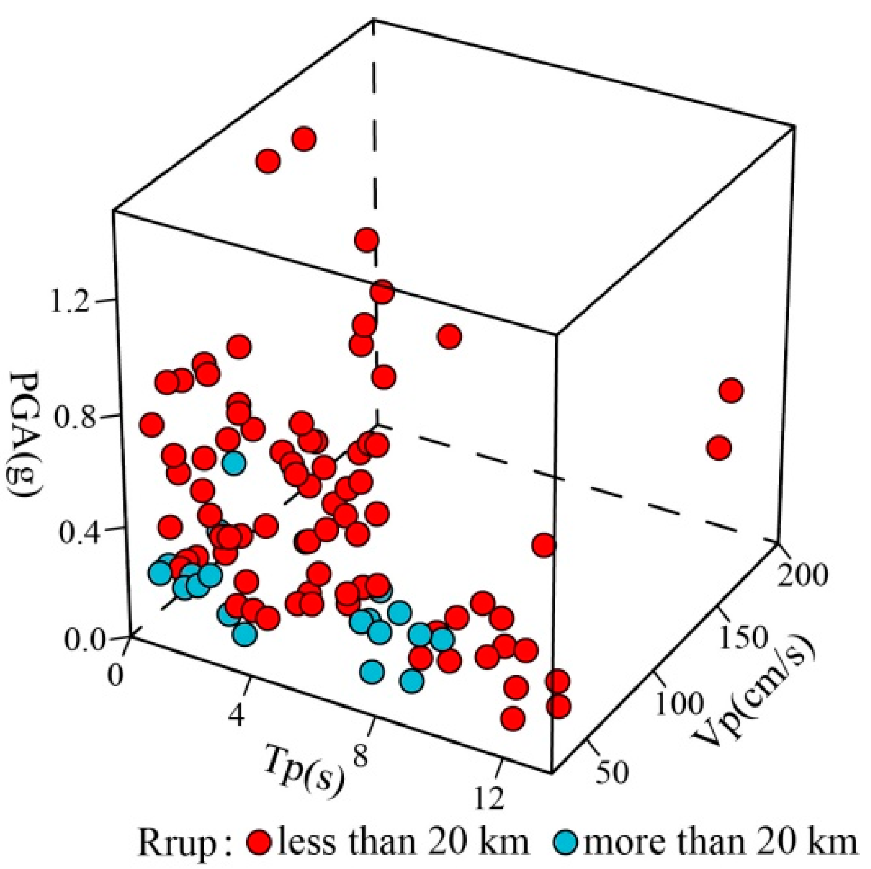
2.1. Selection of Pulse-like Ground Motions

The presence of long-period velocity pulses is a significant characteristic of pulse-like ground motions. The effect of long-period velocity pulses would cause velocity and displacement shocks to any engineering structures in the vicinity, resulting in significant damage that is markedly different from that caused by non-pulse ground motions. Therefore, the selection of pulse-like ground motions is a prerequisite for accurately analyzing the dynamic response of engineering structures. As mentioned above, fault fractures are the main reason for pulse-like ground motions, which is why pulse-like ground motions are usually selected from near-field ground motions with rupture distances of less than 20 km. However, during the propagation of ground motions, when they are passing through complex crustal structures, such as geological basin margins, the velocity pulse effect may also be caused by constructive interference from ground motions.

Baker [27] proposed the wavelet analysis approach to quantitatively identify whether a ground motion contains a velocity pulse. Since the wavelet analysis approach is fully quantitative, reproducible, and inexpensive in terms of computational expense, this approach has been widely used in pulse-like ground motion identification. Using the wavelet analysis approach, Baker identified 91 pulse-like ground motions, and detailed information on these pulse-like ground motions is reported in the literature [27]. Hence, based on these 91 pulse-like ground motions, for this study, we have selected 9 additional pulse-like ground motions from the PEER NGA-West2 database using the wavelet analysis approach. This has led to the number of selected pulse-like ground motions reaching 100, and detailed information regarding the 9 additional pulse-like ground motions is given in

Table 1. Data for the additional pulse-like ground motions.

Number	Time (Year)	Event	Station	Mag	Tp (s)	Vp (cm/s)	Rrup (km)
1	1999	Chi-Chi, Taiwan	TCU052	7.6	12.55	172.34	0.70
2	2004	Parkfield-02, CA	Parkfield—Fault Zone 1	6.0	1.06	81.40	2.50
3	1986	San Salvador	National Geografical Inst	5.8	1.02	73.01	7.00
4	1989	Loma Prieta	Los Gatos—Lexington Dam	6.9	1.69	95.86	5.00
5	1979	Imperial Valley-06	El Centro—Meloland Geot. Array	6.5	3.56	92.62	0.10
6	1992	Cape Mendocino	Bunker Hill FAA	7.0	5.63	67.88	12.20
7	1979	Montenegro, Yugo	Ulcinj—Hotel Olimpic	7.1	1.90	51.64	5.80
8	1992	Cape Mendocino	Centerville Beach, Naval Fac	7.0	1.91	49.55	18.30
9	1995	Kobe, Japan	Port Island (0 m)	6.9	2.83	90.69	3.30

Note: Mag represents seismic magnitude, Tp represents the pulse period of pulse-like ground motions, Vp represents the pulse amplitude of pulse-like ground motions, and Rrup represents the fault distance of pulse-like ground motions.

. The relationship between the peak acceleration, pulse period, pulse amplitude, and fault distance of the selected 100 pulse-like ground motions is shown in Figure 1, and the response spectra are shown in Figure 2.

It can be seen from Figure 1 that the value range of the peak ground acceleration (PGA) of the selected 100 pulse-like ground motions in this study is 0.09–1.44 g, while the value range of the pulse period is from 0.40 s to 12.94 s, the value range of the pulse amplitude is from 30.02 cm/s to 191.17 cm/s, and the maximum fault distance reaches 102.39 km. In addition, there are a total of 19 pulse-like ground motions with a fault distance greater than 20.0 km among the selected 100 pulse-like ground motions. Although the PGA of these ground motions is relatively low, the range of pulse period and pulse amplitude values is 0.79–9.11 s and 30.02–69.96 cm/s, respectively. This indicates that the pulse eigenvalues of far-field pulse-like ground motions are not smaller than those of near-field pulse-like ground motions. Hence, when selecting pulse-like ground motions, it is not advisable to limit the selection to near-field ground motions with fault distances of less than 20 km.

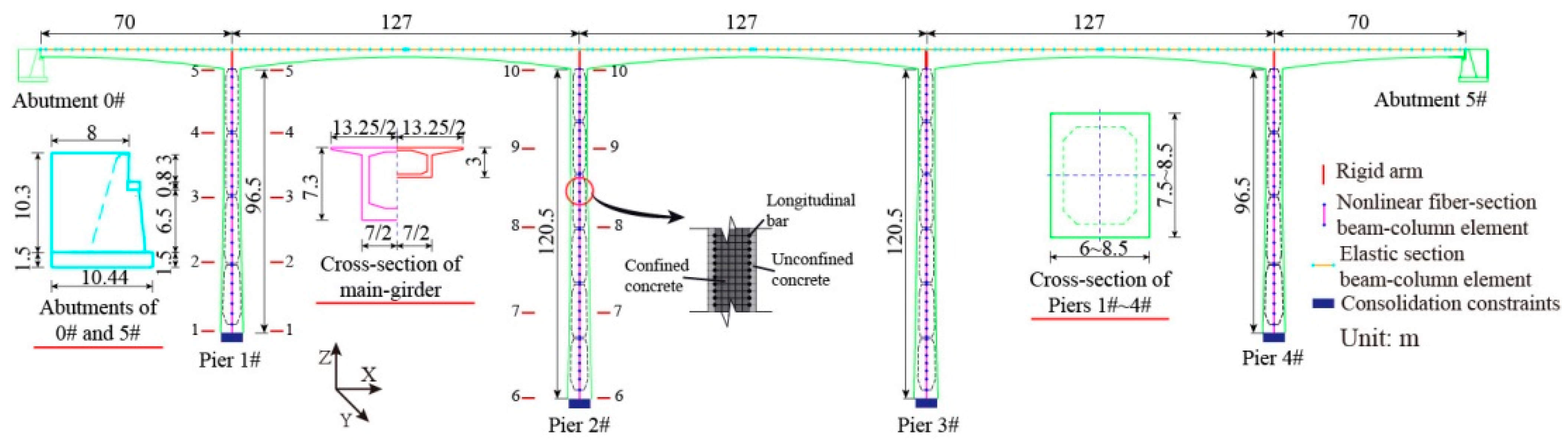
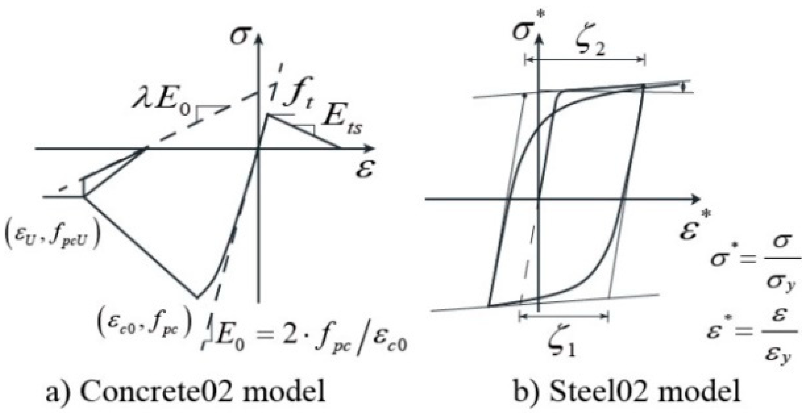
2.2. Engineering Background and Finite Element Modeling

This study employs a practical five-span high-pier prestressed continuous rigid-frame bridge in China with a span arrangement of (70 + 3 × 127 + 70) m for this analysis, as shown in Figure 3. The main girder of this bridge is a single-box and single-chamber prestressed concrete box-girder, with a height of 7.3 m at the pier’s top cross-section gradient, moving to 3.0 m at the mid-span cross-section according to a 1.8 times parabolic curve, constructed using C50 concrete. Piers numbered 1# to 4# are all variable cross-section hollow thin-wall piers made from reinforced C40 concrete; the longitudinal bar and stirrup all use HRB335 steel bars. Meanwhile, both abutments, 0# and 5#, are integral abutments with expanded foundations, and the abutment bearings use GPZ (II) 3.5DX and GPZ (II) 3.5SX pot-type rubber bearings. The detailed geometry of this multi-span high-pier continuous rigid-frame bridge can be seen in Figure 3.

To analyze the dynamic nonlinear response of this five-span high-pier continuous rigid-frame bridge under the influence of pulse-like ground motions, a 3D finite element model was established using OpenSees to conduct a numerical simulation. We used a displacement-based beam-column element combined with an elastic section to simulate the main girder, and the main piers (Piers 1# to 4#) were simulated with a nonlinear beam-column element combined with a fiber section, using a flexibility-based method. To simulate the pier-girder consolidation effect, rigid arms were employed to connect the main girder and the main piers in the analysis. The fiber section of the main pier was discretized into unconfined concrete fibers, confined concrete fibers, and longitudinal bar fibers, with unconfined and confined concrete being simulated using the Concrete02 model [28] and the longitudinal bars simulated using the Steel02 model. In addition, the force–deformation relationship between the Concrete02 model and Steel02 model can be seen in Figure 4. The secondary dead load and self-weight effects of the bridge were simulated using nodal mass points, while the consolidation constraints were used to simulate the boundary conditions at the bottom of the main piers. Meanwhile, the spring abutment modeling method was adopted in this study to establish an abutment model of abutments 0# and 5# to accurately simulate the interaction between the backfill behind the abutment, the abutment, and the main girder, as shown in Figure 5. Detailed descriptions of the modeling method for the spring abutment model of a five-span continuous rigid frame bridge can be found in the literature [9].

3. Correlation Analysis of Seismic IMs

3.1. Initial Candidate Seismic IMs

The appropriateness of selecting a seismic IM is an important factor affecting the accuracy of structural seismic damage assessment. If too many seismic IMs are selected, some of them may have a similar failure mechanism to that of engineering structures or strong correlations with other IMs, which may make it difficult to accurately evaluate the dynamic damage experienced by engineering structures. Moreover, selecting too few seismic IMs may prevent a comprehensive and accurate evaluation of the correlation between ground motion and structural seismic damage. Therefore, to ensure accuracy and comprehensiveness, IMs that can reflect the amplitude, spectral characteristics, and duration of ground motion should be selected from a comprehensive range of IMs. In this study, 29 seismic IMs, shown in

Table 2. The initial candidate seismic IMs.

Intensity Measure		Description	Unit	Intensity Measure		Description	Unit
1	PGA	Peak ground acceleration	cm/s2	16	Arms	Housner root mean square measure	cm/s2
2	PGV	Peak ground velocity	cm/s	17	ASI	Acceleration spectrum intensity	cm/s
3	PGD	Peak ground displacement	cm	18	VSI	Velocity spectrum intensity	cm
4	PGV/PGA	Peak ground velocity to peak ground acceleration ratio	s	19	DSI	Displacement spectrum intensity	cm‧s
5	PGD/PGV	Peak ground displacement to peak ground velocity ratio	s	20	IAM	Modified Arias intensity	cm/s
6	SI	Housner intensity	cm	21	IF	Fajfar measure	/
7	aRMS	Root mean square of acceleration	cm/s2	22	Tp	Velocity pulse period	s
8	vRMS	Root mean square of velocity	cm/s	23	Vp	Velocity pulse amplitude	cm/s
9	dRMS	Root mean square of displacement	cm	24	Samax	Peak acceleration spectrum	cm/s2
10	Td	The interval of time between the 5% and 95% thresholds of the total Arias intensity	s	25	Svmax	Peak velocity spectrum	cm/s
11	IA	Arias intensity	cm/s	26	Sdmax	Peak displacement spectrum	cm
12	IC	Characteristic intensity	/	27	Sa(T1)	Spectral acceleration at first mode period	cm/s2
13	SED	Specific energy density	cm2/s	28	Sv(T1)	Spectral velocity at first mode period	cm/s
14	CAV	Cumulative absolute velocity	cm/s	29	Sd(T1)	Spectral displacement at first mode period	cm
15	CAD	Cumulative absolute displacement	cm

, were selected as the initial candidate seismic IMs.

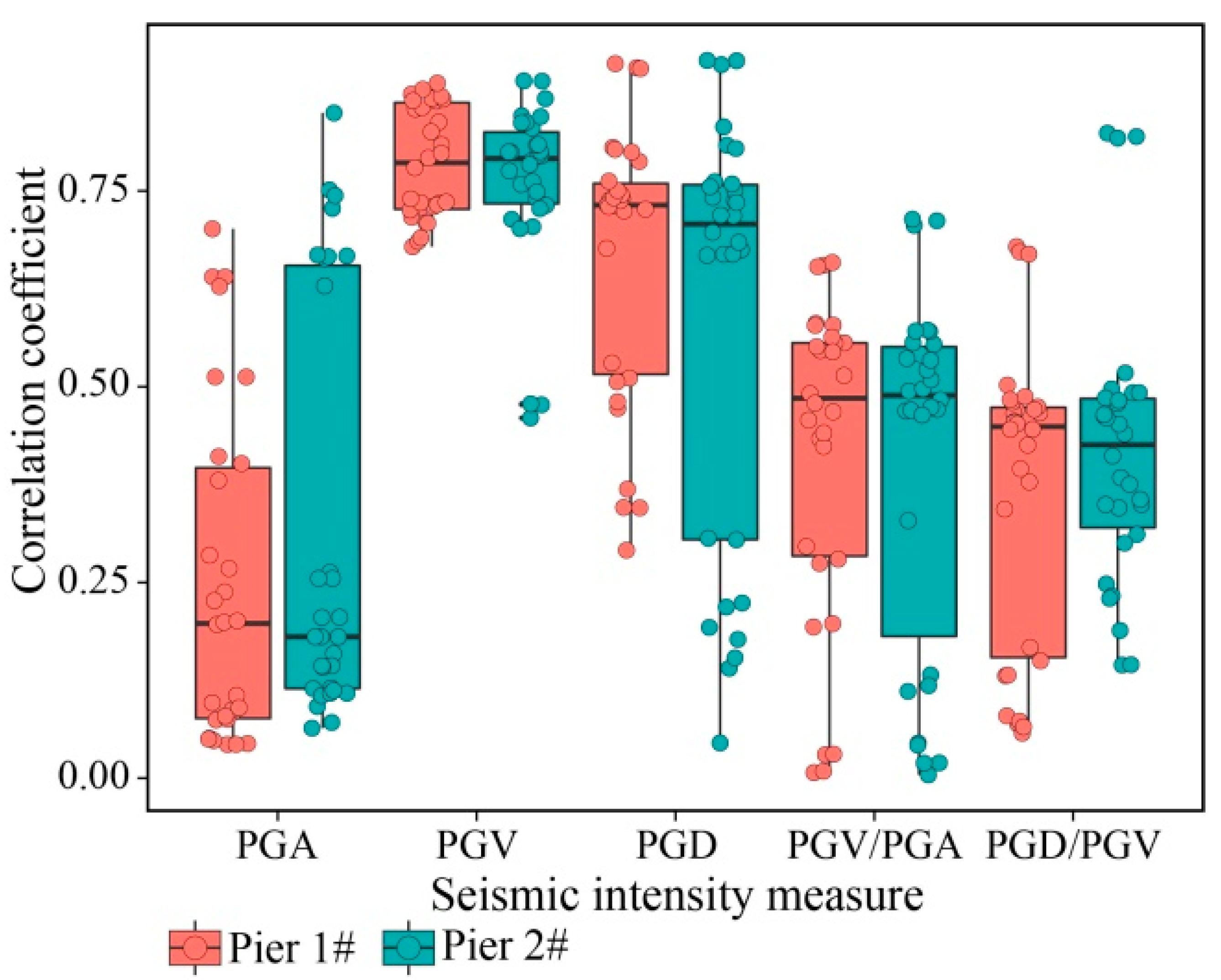
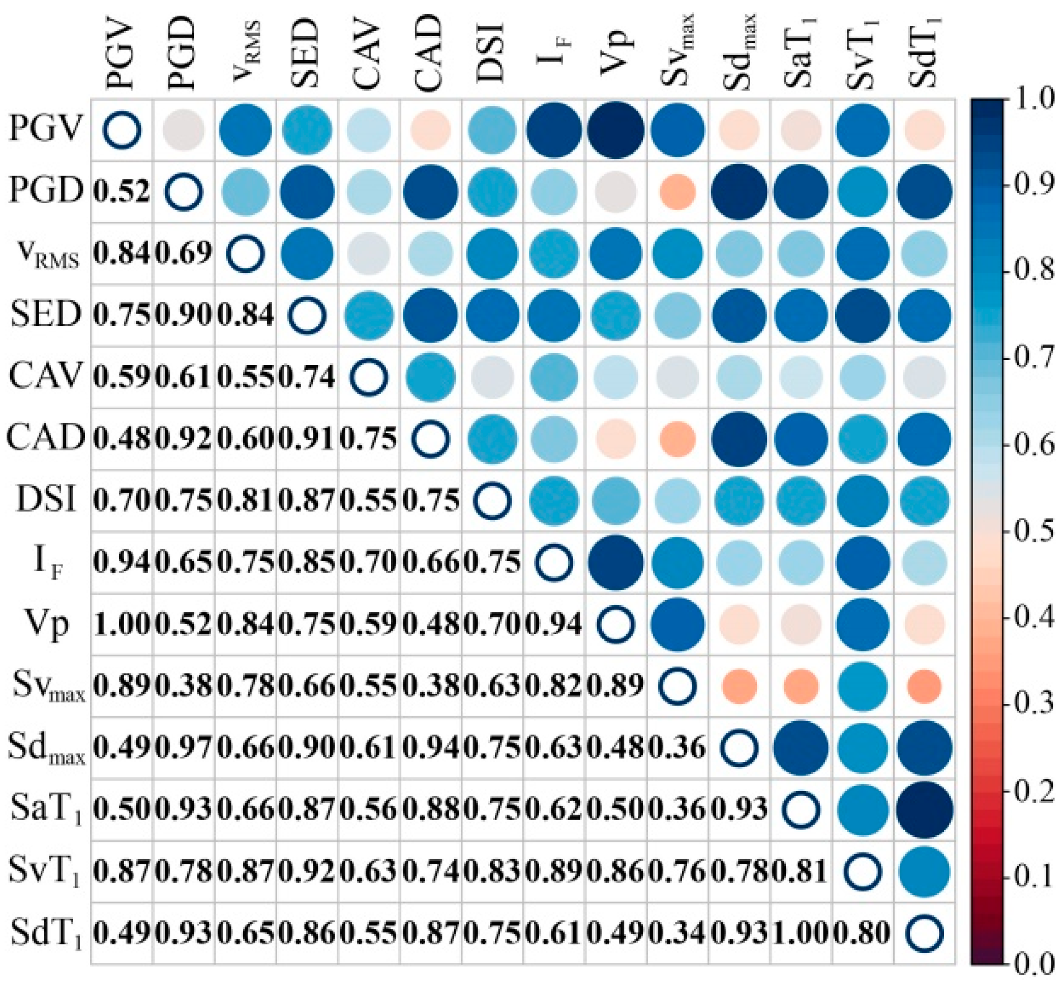
3.2. Correlation Analysis between Seismic IMs

The correlation coefficient is a statistical indicator used to evaluate the degree of correlation between two variables. Currently, the most commonly used correlation coefficients include the Pearson correlation coefficient, Spearman correlation coefficient, and Kendall correlation coefficient. Among them, the Pearson correlation coefficient is commonly used to evaluate the correlation between two continuous variables that follow a normal distribution and have a linear relationship; the Spearman correlation coefficient is a rank correlation coefficient, which does not require variables to follow a normal distribution and can describe the nonlinear correlation between two variables; the Kendall correlation coefficient is suitable for measuring the correlation between two ordinal categorical variables and evaluates the correlation according to the consistency of the ordered pairs between the two variables. Since the data of various IMs may not conform to a normal distribution, and the calculation method of the Kendall correlation coefficient is relatively complicated, the authors of this study ultimately decided to adopt the Spearman correlation coefficient to evaluate the correlation between each IM. The Spearman correlation coefficient between each initial candidate seismic IM is calculated according to Equation (1):

$${\rho }_s=1-\frac{6{\displaystyle \sum _{k=1}^n{(I{M}_{i,k}-I{M}_{j,k})}^2}}{n(n^2-1)}$$

(1)

where $n$ is the number of selected ground motions, herein $n=100$; $I{M}_{i,k}$ is the rank of the i-th $(i=1,2,\dots ,29)$ seismic IM in sample $(I{M}_{i,1},I{M}_{i,2},\dots ,I{M}_{i,100})$; $I{M}_{j,k}$ is the rank of the j-th $(j=1,2,\dots ,29)$ seismic IM in sample $(I{M}_{j,1},I{M}_{j,2},\dots ,I{M}_{j,100})$.

According to the absolute value of the Spearman correlation coefficient, the degree of correlation between seismic IMs can be divided into three levels: when $\left|{\rho }_s\right|=0.0~0.3$, this indicates that the correlation degree between two seismic IMs is low; when $\left|{\rho }_s\right|=0.6~1.0$, this indicates a significant correlation between two seismic IMs; when $\left|{\rho }_s\right|=0.6~1.0$, this indicates that the two seismic IMs are highly correlated. Therefore, this study first calculates the values of 29 IMs for the 100 pulse-like ground motions discussed in Section 2.1, and then calculates the Spearman correlation coefficients between the 29 seismic IMs according to Equation (1), as shown in Figure 6.

As can be seen from Figure 6, the correlation coefficient values among the 29 initial candidate IMs have a wide distribution. Notably, the correlation coefficient values between PGV and Vp, as well as between Arms and a_RMS, are both 1.0, indicating that these IMs are completely correlated. The correlation coefficient value between d_RMS and I_C is the smallest at only 1.2 × 10⁻⁴, close to zero, indicating that d_RMS and I_C are almost completely uncorrelated. This further illustrates that the 29 initial candidate IMs in Section 3.1 are relatively comprehensive and are suitable as initial candidates for seismic IMs.

4. Selection of Seismic IMs for the PCA Algorithm

It can be seen from above that the 29 initial candidate seismic IMs selected in Section 3.1 are relatively comprehensive, reducing the possibility of missing important ground motion information. However, if the 29 IMs are used directly for PCA analysis, the large number of variables would increase the complexity of PCA analysis. Additionally, some IMs are completely correlated, which increases the likelihood of information overlap and masks the real properties of the ground motions. On the other hand, some seismic IMs may have absolutely no correlation with each other, making them unsuitable for use with the PCA algorithm. Therefore, in accordance with these characteristics of the PCA analysis method, the weakly correlated and multicollinearity IMs among the 29 initial candidate seismic IMs should be eliminated, thereby ascertaining a combination of seismic IMs that achieves a balance between computational efficiency and accuracy in the PCA algorithm.

4.1. PCA Algorithm

The PCA algorithm was first proposed by Pearson [29] in 1901 and was then extended to random variables by Hotelling [30] in 1933; it is currently a commonly used data dimensionality reduction method. PCA utilizes a method that converts multiple variables into several principal components through dimensionality reduction techniques. These principal components are new variables that are composed of linear combinations of the original variables and that retain most of the information from the original variables. Moreover, the PCA algorithm does not require the data distribution to be taken into account.

Assuming that there is a total of $n$ pulse-like ground motions and the $p$ seismic IMs are selected, i.e., each seismic IM has $n$ data, therefore, a seismic IM matrix of $n\times p$ dimensions can be formed:

$$\begin{array}{ll}IM& =\left[\begin{array}{cccc}I{M}_{1,1}& I{M}_{1,2}& \cdots & I{M}_{1,p}\\ I{M}_{2,1}& I{M}_{2,2}& \cdots & I{M}_{2,p}\\ ⋮& ⋮& & ⋮\\ I{M}_{n,1}& I{M}_{n,2}& \cdots & I{M}_{n,p}\end{array}\right]\\ & =\left[\begin{array}{cccc}I{M}_1& I{M}_2& \cdots & I{M}_p\end{array}\right]\end{array}$$

(2)

where $I{M}_{i,j}$ is the j-th $\left(j=1,2,\cdots ,p\right)$ seismic IM of the i-th $\left(i=1,2,\cdots ,n\right)$ ground motion, and $I{M}_j$ is the j-th vector of seismic IM, $I{M}_j={\left[\begin{array}{cccc}I{M}_{1,j}& I{M}_{2,j}& \cdots & I{M}_{n,j}\end{array}\right]}^T\left(j=1,2,\cdots ,p\right)$.

Due to the differing measurement units of various IMs, there may be significant differences in the values of some IMs. Therefore, in accordance with Equation (3), each seismic IM vector is standardized to eliminate differences in both the magnitude order and dimensions between each seismic IM:

$$I{M}_{i,j}^{\prime }=\frac{I{M}_{i,j}-{\mu }_j}{\sqrt{s_j}}$$

(3)

where $M_{i,j}^{\prime }$ is the j-th seismic IM value of the i-th ground motion after standardization processing; ${\mu }_j$ is the mean value of the j-th seismic IM vector, ${\mu }_j={\displaystyle \sum _{i=1}^{n}I{M}_{i,j}}/n$; $s_j$ is the sample variance of the j-th seismic IM vector, $s_j={\displaystyle \sum _{i=1}^n{\left(I{M}_{i,j}-{\mu }_j\right)}^2}/\left(n-1\right)$.

After undergoing standardized processing, the IM matrix in Equation (2) is transformed into:

$${\mathit{IM}}^{\prime }=\left[\begin{array}{cccc}{\mathit{IM}}_1^{\prime }& {\mathit{IM}}_2^{\prime }& \cdots & {\mathit{IM}}_p^{\prime }\end{array}\right]$$

(4)

where ${\mathit{IM}}_j^{\prime }$ is the vector of j-th seismic IM value after standardized processing, ${\mathit{IM}}_j^{\prime }={\left[\begin{array}{cccc}{\mathit{IM}}_{1,j}^{\prime }& {\mathit{IM}}_{2,j}^{\prime }& \cdots & {\mathit{IM}}_{n,j}^{\prime }\end{array}\right]}^T$.

According to the standardized IM matrix ${\mathit{IM}}_j^{\prime }$, the correlation coefficient matrix, $R$, can be obtained as:

$$R=\left[\begin{array}{l}\begin{array}{cccc}{r}_{1,1}& r_{1,2}& \cdots & r_{1,p}\end{array}\\ \begin{array}{cccc}{r}_{2,1}& r_{2,2}& \cdots & r_{2,p}\end{array}\\ ⋮\\ \begin{array}{cccc}{r}_{p,1}& r_{p,2}& \cdots & r_{p,p}\end{array}\end{array}\right]$$

(5)

where $r_{l,m}$ is the correlation coefficient between the l-th and m-th seismic IM, $r_{l,m}={\displaystyle \sum _{k=1}^n\left({\mathit{IM}}_{k,l}^{\prime }-I{\mathit{IM}}_{k,m}^{\prime }\right)}/\left(n-1\right)\left(l,m=1,2,\cdots ,p\right)$.

If we calculate the eigenvalues ${\lambda }_1\ge {\lambda }_2\ge \cdots \ge {\lambda }_p$ and corresponding eigenvectors ${\mu }_1,{\mu }_2,\cdots {\mu }_p$ of the correlation coefficient matrix $R$, where ${\mu }_l={\left[\begin{array}{cccc}{\mu }_{l,1}& {\mu }_{l,2}& \cdots & {\mu }_{l,p}\end{array}\right]}^T\left(l=1,2,\cdots ,p\right)$, then, new $p$ variables can be obtained:

$$\left\{\begin{array}{l}{F}_1={\mu }_{1,1}{\mathit{IM}}_1^{\prime }+{\mu }_{2,1}{\mathit{IM}}_2^{\prime }+\cdots +{\mu }_{p,1}{\mathit{IM}}_p^{\prime }\\ F_2={\mu }_{1,2}{\mathit{IM}}_1^{\prime }+{\mu }_{2,2}{\mathit{IM}}_2^{\prime }+\cdots +{\mu }_{p,2}{\mathit{IM}}_p^{\prime }\\ \begin{array}{cccc}& & & ⋮\end{array}\\ F_p={\mu }_{1,p}{\mathit{IM}}_1^{\prime }+{\mu }_{2,p}{\mathit{IM}}_2^{\prime }+\cdots +{\mu }_{p,p}{\mathit{IM}}_p^{\prime }\end{array}\right.$$

(6)

where $F_1$ is the first principal component, $F_2$ is the second principal component, $\cdots$, and $F_p$ is the p-th principal component.

From the above calculations, it can be seen that the principal component is a special linear combination of the $p$ seismic IM vectors. Each principal component is uncorrelated with the others, giving the principal component superior performance compared to the original variable, simplifying the system structures, and capturing the essence of problems. Meanwhile, the contribution rate and cumulative contribution rate of each principal component can be calculated according to Equations (7) and (8):

$${\omega }_l={\lambda }_l/{\displaystyle \sum _{k=1}^p{\lambda }_k}$$

(7)

$$Q_l={\displaystyle \sum _{k=1}^l{\lambda }_k}/{\displaystyle \sum _{k=1}^p{\lambda }_k}$$

(8)

where $a_l$ is the contribution rate of the l-th principal component, $Q_l$ is the cumulative contribution rate of the first l principal components, and ${\lambda }_l$ is the l-th eigenvalue.

The purpose of using PCA in this study is to simplify the selected $p$ seismic IMs into a few comprehensive variables that can reflect as much ground motion information as possible, with less information loss. Consequently, the first $l\left(l<p\right)$ principal components $F_1$, $F_2$, $\cdots$, and $F_l$, with a cumulative contribution rate, $Q_l$, of no less than 85% as the comprehensive variable, were used in order to reduce the number of IMs and simplify the problem.

4.2. Removal of Weakly Correlated IMs

The PCA algorithm is ideal for reducing the dimensionality of variables with a strong correlation; however, the PCA algorithm is unlikely to achieve satisfactory dimensionality reduction results when the absolute value of the correlation coefficient between variables is less than 0.3. Consequently, this study will remove the weakly correlated IMs, although the correlation coefficient still represents the correlation between two IMs. However, at present, there are no clear evaluation criteria by which to judge which of the two IMs should be removed. Therefore, the correlation between the IMs and the maximum cross-section curvature values of high piers under seismic loading is used as the evaluation standard in this study. Based on the evaluation standard, the IM that has less correlation coefficient value with the maximum cross-sectional curvature values among the two weakly correlated IMs would be removed.

In this section, the key cross-sections selected for analysis include the bottom cross-sections of Pier 1# and Pier 2# (cross-sections 1-1 and 6-6), the one-quarter-height cross-sections of Pier 1# and Pier 2# (cross-sections 2-2 and 7-7), the mid-height cross-sections of Pier 1# and Pier 2# (cross-sections 3-3 and 8-8), the three-quarter-height cross-sections of Pier 1# and Pier 2# (cross-sections 4-4 and 9-9), and the top cross-sections of Pier 1# and Pier 2# (cross-sections 5-5 and 10-10), as shown in Figure 3. This study will then conduct nonlinear dynamic time–history analyses (NDTHA) for a five-span continuous rigid-frame bridge (as shown in Section 2.2) under the influence of the following four pulse-like ground motion excitation calculation cases:

(1)

A longitudinal earthquake;

(2)

A transverse earthquake;

(3)

A biaxial earthquake (longitudinal direction + transverse direction);

(4)

A triaxial earthquake (longitudinal direction + transverse direction + vertical direction).

According to the GB 50011-2010 code [31], the PGA of triaxial ground motions is regulated in the following ratio: longitudinal direction:transverse direction:vertical direction = 1:0.85:0.65.

By recording the maximum cross-sectional curvature values of each key cross-section for each calculated case, this study calculates the Spearman correlation coefficient values between each IM of each pulse-like ground motion (selected in Section 2.1) and the maximum cross-sectional curvature of each key cross-section, using Equation (9). Furthermore, upon analyzing the correlation coefficient values between the IMs and the key cross-section curvature values of high piers, it was found that the correlation coefficient values corresponding to the same IM were inconsistent, and some of the correlation coefficient values were even dispersed to a large extent, as shown in Figure 7. Due to space limitations, Figure 7 only represents the correlation coefficient values between 5 IMs, comprising PGA, PGV, PGD, PGV/PGA, and PGD/PGV, and the cross-sectional curvature values of Pier 1# and Pier 2#:

$$\rho =1-\frac{6{\displaystyle \sum _{k=1}^n{(I{M}_{i,k}-{\phi }_{l,m,k})}^2}}{n(n^2-1)}$$

(9)

where ${\phi }_{l,m,k}$ is the cross-sectional curvature value of the l-th $(l=1,2,\dots ,10)$ key cross-section under the influence of k-th $(k=1,2,\dots ,100)$ of ground motion of the m-th $(m=1,2,3,4)$ calculated case.

It can be seen from Figure 7 that the mean value of the correlation coefficients corresponding to PGV is the largest and the discreteness is the smallest, yet the mean values of the correlation coefficients of the other 4 IMs are all smaller than PGV, and the dispersion is relatively large. This is especially applicable to the mean value of the correlation coefficients corresponding to PGA, which is commonly used in seismic fragility analysis. It is the smallest value among the 5 IMs and the discreteness of the correlation coefficient values is the largest.

Hence, this study first calculates the Spearman correlation coefficients between the 29 IMs selected in Section 3.1 and then picks out those IMs where the correlation coefficients are less than 0.3. Then, the correlation coefficient values between the selected IMs and the key cross-section curvatures of Pier 1# and Pier 2# are calculated, and, in the meantime, the mean values and the standard deviation values of the correlation coefficients of each chosen IM are obtained via the statistical approach. After this, through comprehensive and comparative analysis of the mean values and the standard deviation values of the weakly correlated IMs, the IMs with smaller means and larger dispersion are determined and removed. After the above processing, a total of 14 IMs are eventually selected; the correlation coefficients between the various IMs are shown in Figure 8. It can be seen from Figure 8 that the minimum value of the correlation coefficient among the remaining 14 IMs is 0.34, and there are no weakly correlated IMs.

4.3. Elimination of Multicollinearity IMs

Multicollinearity was first proposed by the statistician, Frisch, in 1934, and refers to the phenomenon of different independent variables in a model being highly correlated with each other. This multicollinearity means that the different IMs repeatedly describe a certain characteristic of ground motions. This will result in the overemphasis of certain characteristics of ground motions, affect the objectivity of the analysis, and compromise its accuracy and reliability. To overcome the adverse effects of overlapping information caused by multicollinearity, it is recommended to eliminate those IMs that exhibit high levels of multicollinearity.

For the remaining 14 IMs, after removing the weakly correlated IMs in Section 4.2, if there are 15 parameters $c_0,c_1,\cdots ,c_{14}$, the following equation can be obtained:

$$c_0+c_{1}I{M}_{i,1}+c_{2}I{M}_{i,2}+\cdots +c_{14}I{M}_{i,14}\approx 0\left(i=1,2,\cdots ,100\right)$$

(10)

There appears to be multicollinearity among the seismic IMs ($I{M}_1,I{M}_2,\cdots ,I{M}_{14}$). The vector form of the seismic IMs of Equation (10) can be expressed as:

$$c_{0}I{M}_0+c_{1}I{M}_1+c_{2}I{M}_2+\cdots +c_{14}I{M}_{14}={\mathit{IM}}^{\prime }c\approx 0$$

(11)

where $I{M}_0$ is a 100 × 1 dimensional column vector where all elements are equal to 1, $I{M}_0={\left[\begin{array}{cccc}1& 1& \cdots & 1\end{array}\right]}^T$; $c$ is a unit eigenvector, $c={\left[\begin{array}{cccc}{c}_1& c_2& \cdots & c_{14}\end{array}\right]}^T$; $I{M}^{\prime }=\left[\begin{array}{cccc}I{M}_0& I{M}_1& \begin{array}{cc}I{M}_2& \cdots \end{array}& I{M}_{14}\end{array}\right]$.

As suggested in the literature [32], the condition number $k_i$ can serve as a useful metric for determining the presence of multicollinearity among the remaining 14 IMs, and the condition number $k_i$ can be calculated as follows:

$$k_i=\sqrt{\frac{{\lambda }_{\max }}{{\lambda }_i}}\left(i=1,2,\cdots ,p\right)$$

(12)

where $k_i$ is the condition number, ${\lambda }_{\max }$ is the maximum eigenvalue of the matrix $I{M^{\prime }}^{T}I{M}^{\prime }$, and ${\lambda }_i$ is the i-th eigenvalue of matrix $I{M^{\prime }}^{T}I{M}^{\prime }$.

Generally, it can be considered that when $0<k<10$, there is little multicollinearity; when $10\le k<100$, there is a strong multicollinearity; when $k\ge 100$, there is a severe multicollinearity. To address the issue of multicollinearity among the remaining 14 IMs, this study employs Equation (12) to calculate their condition number. Any seismic IM with a condition number that exceeds 100 is eliminated, as per the study’s methodology.

4.4. Principal Component Analysis of IMs

Following the removal of weakly correlated IMs (Section 4.2) and the elimination of multicollinearity IMs (Section 4.3), the final set of 11 IMs selected for analysis in this study included PGV, PGD, v_RMS, SED, CAV, CAD, DSI, Sv_max, Sd_max, Sv(T₁), and Sd(T₁). The condition numbers of the final set of 11 IMs are shown in Figure 9. Meanwhile, the Spearman correlation coefficient values between the final set of 11 IMs were computed using Equation (1) and are presented in Figure 10.

It can be seen from Figure 9 that the maximum condition number of the final set of 11 IMs is 63.09, indicating that the final set of 11 IMs did not have a severe multicollinearity problem. As shown in Figure 10, the minimum and maximum correlation coefficient values of the final set of 11 IMs are 0.34 and 0.97, respectively, which shows that there are no weakly correlated IMs, and the perfectly correlated IMs have also been removed. As a result, the final set of 11 IMs selected for this study did not exhibit a weak correlation or severe multicollinearity issues. As such, these 11 IMs represent an optimal combination of seismic IMs that meet the requirements for dimensionality reduction analysis using the PCA method.

Taking the final set of 11 IMs, which included PGV, PGD, v_RMS, SED, CAV, CAD, DSI, Sv_max, Sd_max, Sv(T₁), and Sd(T₁), as the basic variables, a seismic IM vector matrix $IM=\left[\begin{array}{cccc}\mathbf{PGV}& \mathbf{PGD}& \cdots & \mathbf{S}\mathbf{d}({\mathbf{T}}_{\mathbf{1}})\end{array}\right]$ was formed. The PCA analysis of the seismic IMs was carried out according to Equations (3)–(6), resulting in 11 uncorrelated principal components $F_1$, $F_2$, $\cdots$, and $F_{11}$, composing the above seismic IM vector. Meanwhile, the contribution rate and accumulated contribution rate of each principal component were calculated according to Equations (7)–(8); the accumulated contribution rate of each principal component is shown in Figure 11.

From Figure 11, it can be seen that the accumulated contribution rate of the first three principal components, $F_1$, $F_2$, and $F_3$, reaches 92%, indicating that the first three principal components could effectively reflect most of the information contained within the final set of 11 IMs. Therefore, this study employed the first three principal components as clustering indices to conduct a clustering analysis, simplifying the high-dimensional variable system into a low-dimensional variable system. Moreover, the variables within the new variable system were all uncorrelated with each other, which not only preserved a significant amount of information related to the seismic IMs but also mitigated the issue of overlapping information between each IM, thereby reducing the complexity of the clustering analysis.

5. Clustering Analysis of the Selected Ground Motions Based on a K-Means Algorithm

5.1. K-Means Clustering Algorithm

The clustering analysis algorithm classifies the object data, based on distance or similarity, which strengthens the similarity between objects of the same class more than that between those of other classes. This maximizes the homogeneity of objects within the same class and the heterogeneity between objects of different classes. Clustering analysis is an important unsupervised learning algorithm and many scholars have conducted extensive research on clustering analysis algorithms. Currently, more than 100 clustering algorithms have been published. Among these clustering algorithms, the K-means clustering algorithm is a dynamic clustering method that is suitable for large-scale data. The K-means clustering algorithm has a simple principle, yielding easy-to-understand analytical results, and does not require high levels of computer performance. It is currently one of the most widely used clustering analysis methods. Therefore, in this study, the K-means clustering algorithm is applied to cluster the original selected group of 100 pulse-like ground motions, using the first three principal components ($F_1$, $F_2$, and $F_3$) as clustering indices, as determined in Section 4.4. The following steps are followed to conduct the clustering analysis:

(1)

Assuming that the ground motions are divided into K initial classes, K data points are randomly selected as the initial clustering centers.

(2)

Assuming that the first three principal component values of ground motion $g_i(i=1,2,\cdots ,100)$ are $(F_{i1},F_{i2},F_{i3})$, and the principal component value of the j-th $(j=1,2,\cdots ,K)$ cluster center is $C_j=(F_{j1},F_{j2},F_{j3})$, then the Euclidean distance $d_{ij}$ between the i-th ground motion and the j-th cluster center is:

$$d(g_i,C_j)=\sqrt{{(F_{i1}-F_{j1})}^2+{(F_{i2}-F_{j2})}^2+{(F_{i3}-F_{j3})}^2}$$

(13)

(3)

Using Equation (13), the Euclidean distance from each ground motion to each cluster center point is calculated separately, and the ground motions are assigned to the nearest cluster center, according to the principle of minimum distance, then the ground motions are classified into K classes;

(4)

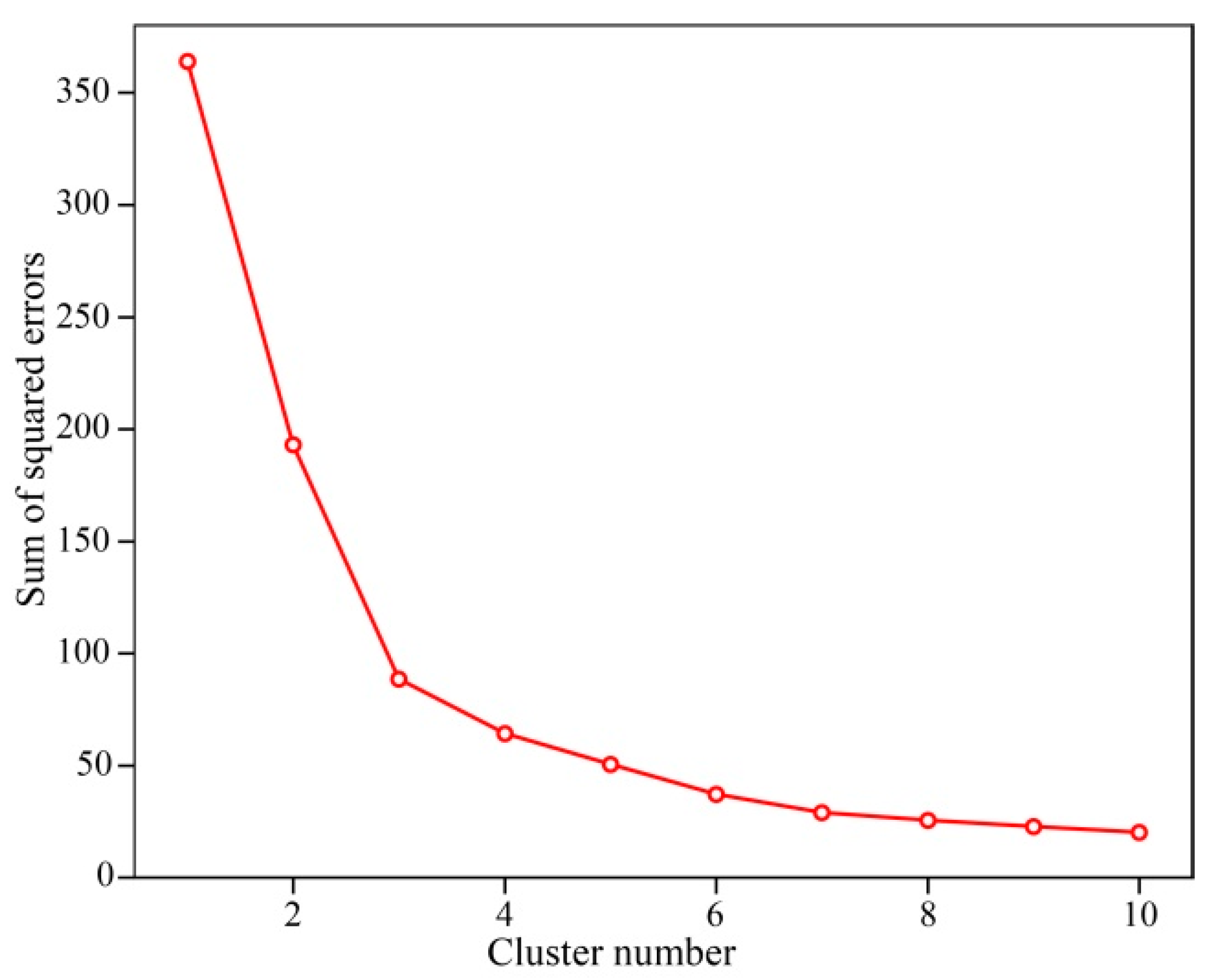
Calculating the sum of squared errors (SSE), $D$, which reflects the distortion degree of clustering, according to Equation (14):

$$D={\displaystyle \sum _{j=1}^K{\displaystyle \sum _{}{(d(G_{lj},C_j))}^2}}$$

(14)

where $G_{lj}$ represents the principal component of the l-th $(l=1,2,\cdots ,n_j)$ ground motion in the j-th class, and $n_j$ represents the number of ground motions in the j-th class.

(5)

Calculating the mean values of the ground motions assigned to each class in step (3) according to Equation (15) and updating the cluster center for each class by using the mean values as the new centroid, then recalculating the sum of squared errors, $D$:

$$m_j=\frac{1}{n_j}{\displaystyle \sum G_{lj}}$$

(15)

where $m_j$ is the mean value of the ground motion data in the j-th class, and $n_j$ is the number of ground motions in the j-th class.

(6)

Performing step (2) to recalculate the Euclidean distance between each ground motion and the updated cluster center in step (5), we then perform step (3) to reclassify each ground motion. We then perform step (5) to update each cluster center point and calculate the sum of squared errors, $D$. We repeat this process until the sum of squared errors has not changed for two consecutive iterations, then terminate the algorithm and output the final cluster analysis results.

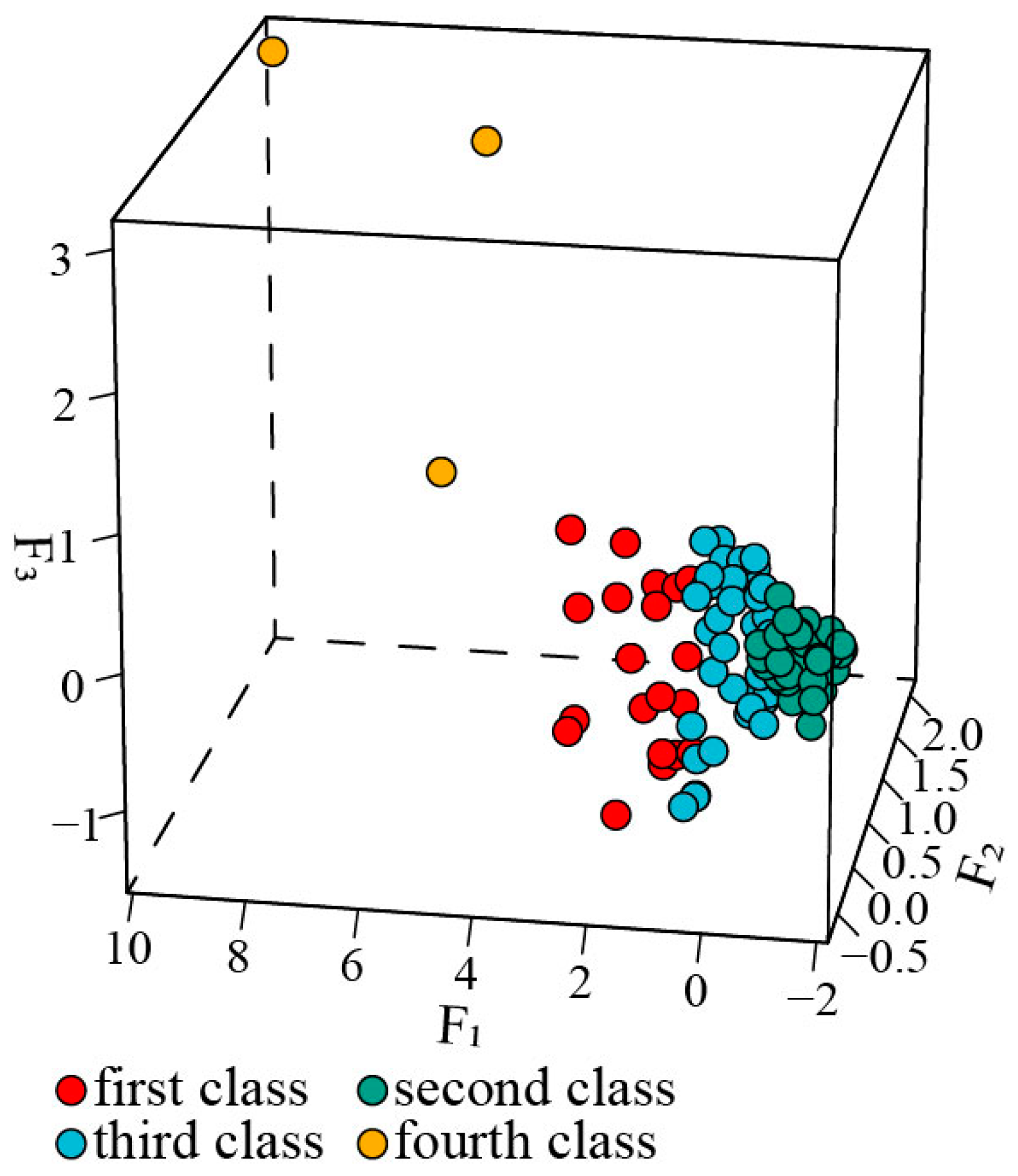
5.2. Pulse-like Ground Motion Clustering Analysis

As shown in Section 5.1, the number of clusters, K, is a crucial problem for the K-means clustering algorithm and directly impacts the final clustering effect. Therefore, an exploratory approach is employed to determine the reasonable number of clusters, K, in this study. Firstly, according to the calculation procedure of the K-means clustering algorithm described in Section 5.1, the initial selected 100 pulse-like ground motions are clustered and analyzed, based on the cluster number K of 1, 2, …, 10, respectively, and the sum of the squared error value, $D$, of each cluster number is calculated. Then, the curve of the relationship between the cluster number and the sum of squared errors is plotted, as shown in Figure 12. The optimal number of clusters for the K-means clustering algorithm is determined by identifying the cluster number corresponding to the point where the slope of the curve changes suddenly from large to small and thereafter changes gradually.

As shown in Figure 12, the slope of the relationship curve decreases significantly once the number of clusters reaches 4, and the rate of change gradually slows down. Thus, the optimal cluster number, K, is determined to be 4; following the analysis steps of the K-means clustering algorithm in Section 5.1, the initial selected pulse-like ground motions are clustered via a K-means clustering algorithm. The clustering analysis results are shown in Figure 13. Meanwhile, it can be seen from Figure 13 that the numbers of pulse-like ground motions in the first class, second class, third class, and fourth class are 20, 38, 39, and 3, respectively. Moreover, the dispersion between each ground motion in the fourth class is relatively large, while the ground motions of the fourth class are obviously far from the ground motions of the other three classes; therefore, it can be classified into one class. Furthermore, the ground motions in the first class, second class, and third class are clustered into cluster shapes, demonstrating the effectiveness of the classification results. It can thus be seen that utilizing the first three principal components of seismic IMs as clustering indices and applying the K-means clustering algorithm for the clustering analysis of pulse-like ground motions can yield highly accurate classification results.

6. Seismic Fragility Analysis of a High-Pier Bridge

6.1. Probability Seismic Fragility Analysis Model

As mentioned earlier, the probabilistic seismic fragility analysis model can reflect the likelihood of a predefined engineering demand parameter (EDP) reaching or exceeding a specific limited stage capacity (LS) for a given seismic IM [33]. Thus, the probabilistic seismic fragility analysis model can be represented as:

$$F_R(x)=P(EDP\ge LS\left|IM\right.)$$

(16)

Based on the assumption of lognormal distribution made by Cornell et al. [34], the damage probability can be calculated as:

$$P(EDP\ge LS\left|IM\right.)=1-\mathsf{\Phi }\left(\frac{\ln (LS)-\ln (EDP)}{{\beta }_{{}_{EDP\left|IM\right.}}}\right)$$

(17)

where $\mathsf{\Phi }(·)$ represents the standard normal cumulative distribution function, and ${\beta }_{{}_{EDP\left|IM\right.}}$ is the conditional logarithmic standard deviation of the engineering demand parameter $EDP$ for the seismic IM.

Meanwhile, the median EDP and the given IM can be calculated approximately, using the following exponential form [34]:

$$\overline{EDP}=a{\left(IM\right)}^b$$

(18)

where $\overline{EDP}$ is the median value of EDP; a and b are the regression coefficients calculated via the least-squares fitting method.

Thus, through logarithmic linear regression, based on the least-squares fitting method, the probabilistic seismic demand model (PSDM) can be represented in the following form:

$$\ln \left(\overline{EDP}\right)=a+b\ln \left(IM\right)$$

(19)

The conditional logarithmic standard deviation ${\beta }_{{}_{EDP\left|IM\right.}}$ can be obtained, as follows:

$${\beta }_{{}_{EDP\left|IM\right.}}=\sqrt{\frac{{\displaystyle \sum _{i=1}^n{\left(\ln (ED{P}_i)-\ln (aI{M}^b)\right)}^2}}{n-2}}$$

(20)

where $n$ is the total number of ground motions.

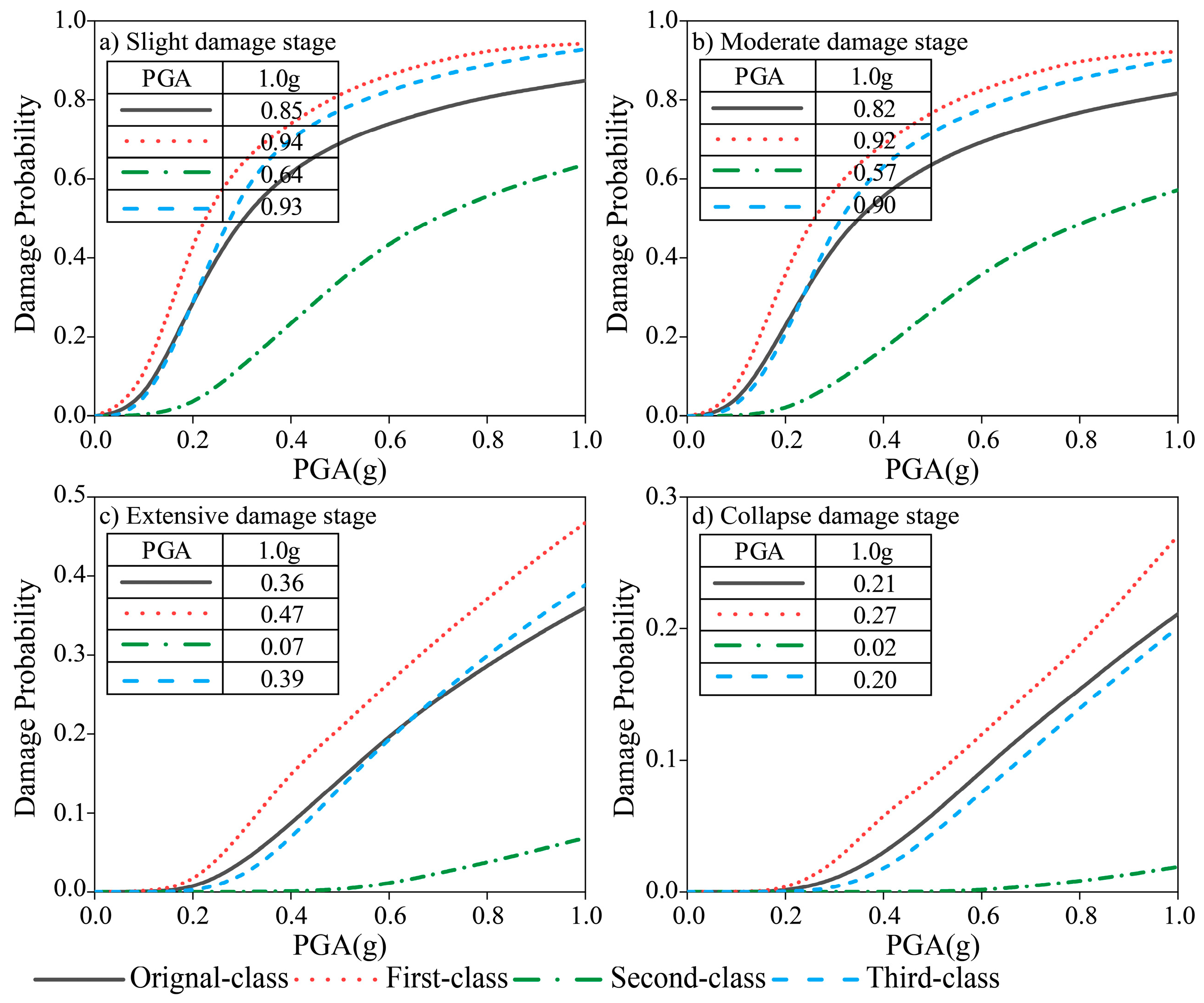
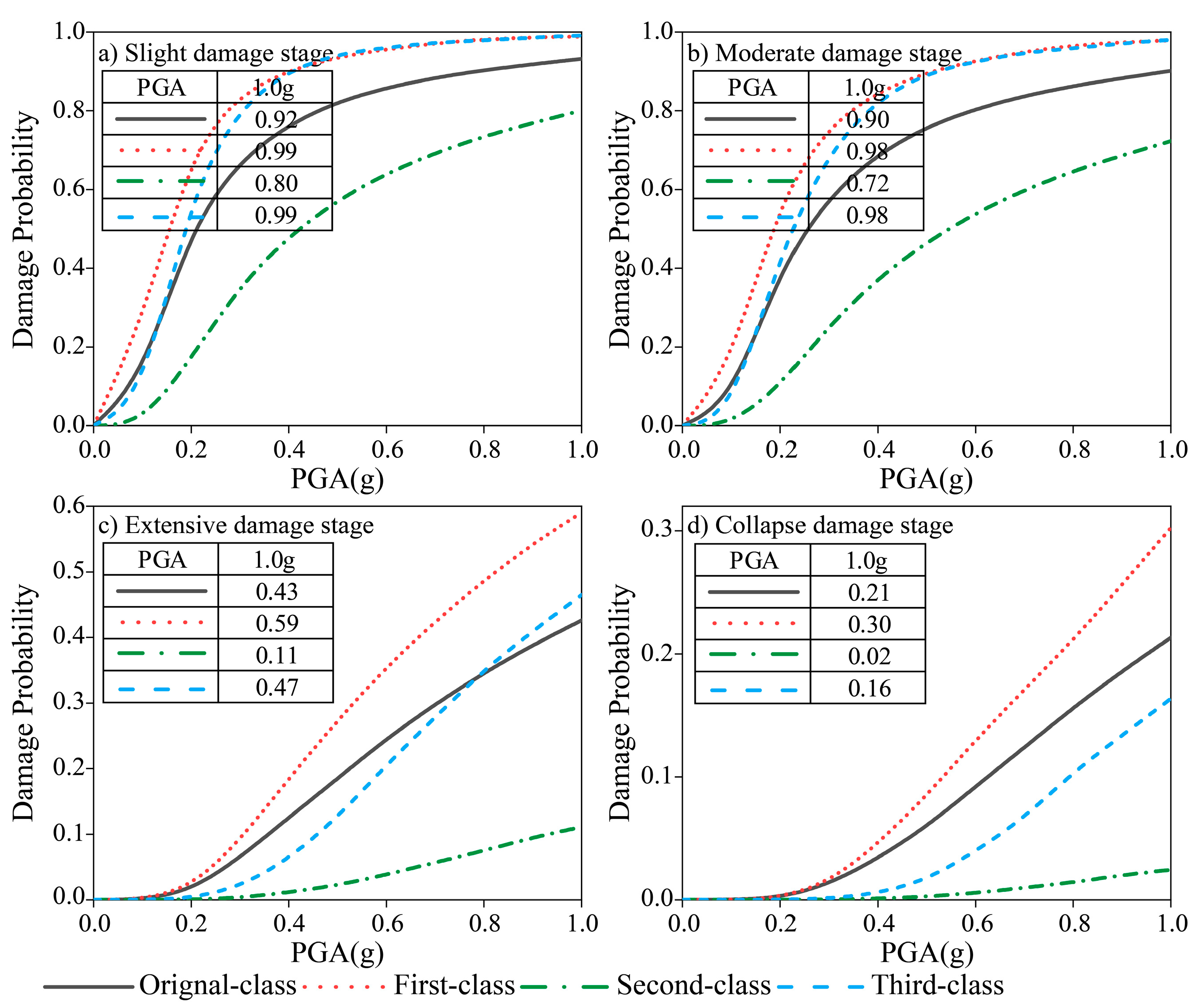
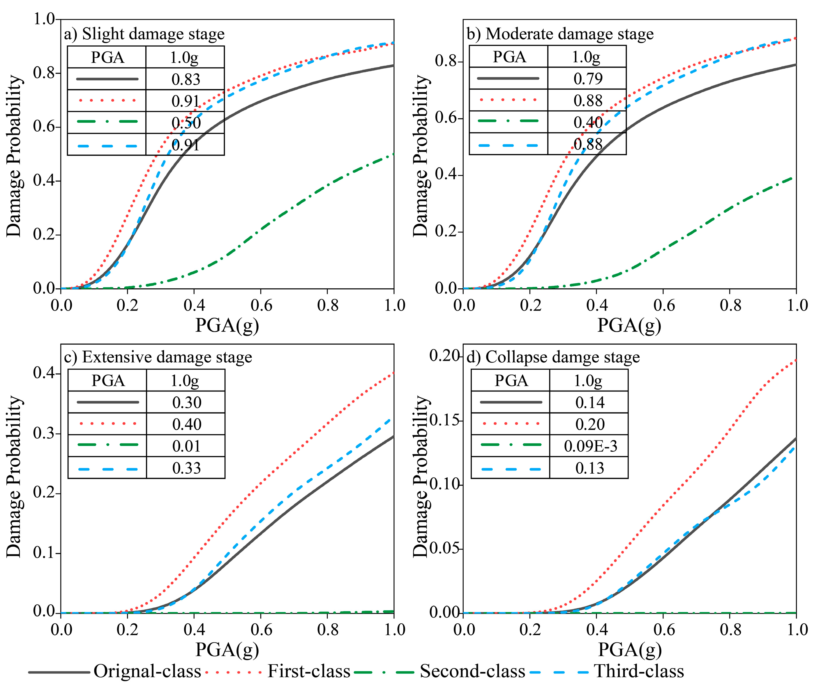
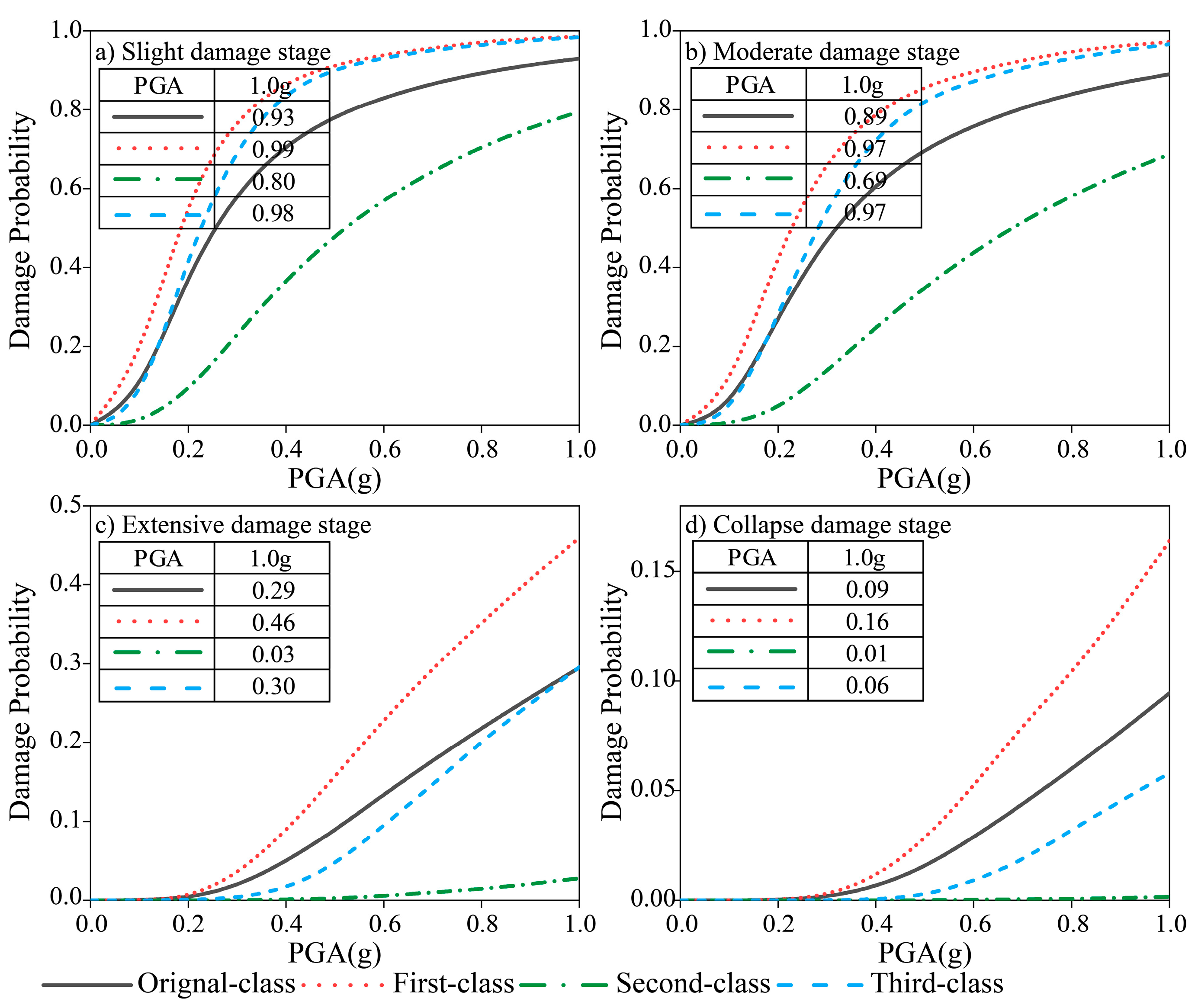
6.2. Seismic Fragility Analysis of the High-Pier Bridge

It can be seen from Equations (16) to (20) that probability seismic fragility analysis is primarily dependent upon the parameters of limited stage capacity, LS, the engineering demand parameter, EDP, and the seismic intensity measure, IM. Previous studies (such as those by the authors of [35]) have shown that there is no synchronous relationship between the curvature of the bottom cross-section and the displacement of the top cross-section for high piers under seismic loading, and the position of the contraflexure point is unstable. It can be seen that the displacement and displacement ductility ratio are not suitable for utilization as LS for assessing the damage characteristics of high piers. Therefore, the cross-sectional curvature is selected as the LS, in order to assess the damage stage of the high piers in this study. The damage stages of high piers are classified into four damage stages, namely, slight, moderate, extensive, and collapsed damage stages, based on the damage stage division standard and the criteria proposed by Zhao et al. [25].

Nowadays, there are two main methods by which to establish the relationship between EDP and IM through nonlinear dynamic time-history analyses (NDTHA) and the probability of the seismic fragility analysis of structures [15,33], namely, the incremental dynamic analysis (IDA) method and the cloud-based analysis method [20,36]. The IDA method requires the selection of a series of ground motions, which are then scaled to generate a range of ground motions with specified intensity levels. Structural finite element models are then subjected to NDTHA under the influence of these scaled ground motions [37,38]. However, unlike the IDA method, the cloud method does not require the scaling of the selected ground motions. Instead, the selected ground motions should demonstrate a wide range of intensity levels and good aleatory uncertainty. As a result, the cloud method can significantly reduce the necessary computational time, compared to the IDA method, as it only requires a few NDTHA runs under the influence of the selected unscaled ground motions [39]. However, to ensure the fitting accuracy of the exponential equation of EDP and IM (as in Equation (18)), the cloud method requires a substantial number of unscaled ground motions to be selected [15]. As shown in Section 5.2, the numbers of the first class, second class, third class, and fourth class of pulse-like ground motions are 20, 38, 39, and 3, respectively. It can be seen that there are only three pulse-like ground motions in the fourth class. Therefore, the pulse-like ground motions in the fourth class should not be used for seismic fragility analysis due to their insufficient number. Meanwhile, the first class consists of only 20 pulse-like ground motions, which is insufficient to meet the requirements of the cloud method. However, 10 to 20 ground motions are sufficient to provide the required accuracy for the IDA method [38]. It can be deduced that the first class, second class, and third class pulse-like ground motions all satisfy the quantity requirement of the IDA method. Moreover, the study published by Zhang and Huo [36] indicates that the IDA method is more accurate than the cloud method in terms of the seismic fragility analysis of bridge structures. Therefore, in this study, we used the IDA method to perform seismic fragility analysis for a five-span high-pier continuous rigid-frame bridge undergoing the original selected 100 pulse-like ground motions (original class), as well as the first class, second class, and third class pulse-like ground motions, respectively.

As shown in Section 4.2, the correlation coefficient values of PGA exhibit a minimum mean value and greater dispersion, indicating that PGA is not the most suitable ground motion intensity measure for the seismic fragility analysis of high-pier bridges. However, due to the ease of obtaining peak ground acceleration values, PGA is one of the earliest and most commonly used indicators for characterizing the intensity of ground motions in seismic studies. Furthermore, as previously mentioned, this study utilized the IDA method to conduct seismic fragility analysis for the research bridge, necessitating the scaling of ground motions to encompass the various levels of specified IM. The ground motion intensity measure, PGA, is commonly selected as the specified IM, and a series of ground motions within a wide range of intensity levels are generated by scaling the PGA values. NDTHA is then conducted at various intensity levels. PGA was identified as the optimum IM by Padgett et al. [40] for performing the seismic fragility analysis of bridge structures. Many studies utilize PGA as the ground motion intensity measure when performing seismic fragility analysis for bridge structures, as in the studies by Zhang and Huo [36] and Chen et al. [41]. Elsewhere, Chen et al. [35] also investigated the variable characteristics of seismic damage probability for a high-pier bridge under various PGA levels. As the primary objective of this study was to investigate and establish the need for utilizing the PCA-K-means method to cluster ground motions and conduct seismic fragility analysis, PGA was chosen as the ground motion IM for analyzing the seismic fragility analysis of the research object, a five-span, high-pier, continuous rigid-framed bridge.

Selecting the bottom cross-sections of Pier 1# and Pier 2# (cross-sections 1-1 and 6-6) and the top cross-sections of Pier 1# and Pier 2# (cross-sections 5-5 and 10-10) as the research cross-sections (as shown in Figure 3), seismic fragility analysis was performed for each research cross-section, subject to the original class and the first class, second class, and third class pulse-like ground motions along the longitudinal direction. The fragility curves for each research cross-section were derived by following the main procedural steps, as follows.

Step 1: Establish the finite element model of the five-span, high-pier, continuous rigid-frame bridge, following the modeling methodology outlined in Section 2.2.

Step 2: The original class, first class, second class, and third class pulse-like ground motions are scaled using PGA and ranging from 0.1 g to 1.0 g, with 0.1 g increments.

Step 3: Perform NDTHA of the finite element model by inputting each class of ground motions along the longitudinal direction to obtain the corresponding maximum cross-sectional curvature values of each research cross-section.

Step 4: Using the Xtract software to calculate the critical curvature values of each damage stage for each research cross-section along the longitudinal direction. The critical cross-sectional curvature values of each research cross-section are shown in the literature [42].

Step 5: According to Equations (17)–(20), the conditional damage probability of each damage stage of each cross-section is calculated, using different PGA levels.

Step 6: Draw the seismic fragility curves for each cross-section along the longitudinal direction, using PGA as the horizontal axis and the conditional damage probability as the vertical axis.

The seismic fragility curves of each damage stage for each research cross-section are shown in Figure 14, Figure 15, Figure 16 and Figure 17.

It can be seen from Figure 14 and Figure 15 that the damage probability to cross-sections 1-1 and 5-5 at each damage stage increased with increasing PGA for each of the original class, first class, second class, and third class pulse-like ground motions. For the bottom cross-section of Pier 1# (cross-section 1-1), when the PGA value reached 1.0 g, the damage probabilities of the slight and moderate damage stages undergoing the first class of ground motions reached maximum values of 0.94 and 0.92, while the damage probabilities of the third class pulse-like ground motions were 0.93 and 0.90. Thus, the fragility curves of the slight and moderate damage stages under the first class and third class ground motions were generally consistent with the increase in PGA, while the damage probability values were larger than the original class pulse-like ground motions. Meanwhile, the damage probability values of the extensive damage stage under the original class and third class pulse-like ground motions eventually reached 0.36 and 0.39, while the damage probabilities of the original class and third class pulse-like ground motions in the collapse damage stage were 0.21 and 0.20 when the PGA value reached 1.0 g. Therefore, in the extensive damage and collapse damage stages, the fragility curves of the original class and third class pulse-like ground motions were basically identical and were all smaller than the damage probability under the first class pulse-like ground motions. In addition, the maximum damage probabilities of the various damage stages under the second class pulse-like ground motions were 0.64, 0.57, 0.07, and 0.02, respectively, while the fragility curves of the second class pulse-like ground motions were lowest among the various classes of pulse-like ground motions.

Meanwhile, as shown in Figure 15, for the top cross-section of Pier 1# (cross-section 5-5), the fragility curves of the slight and moderate damage stages under the first class and the third class pulse-like ground motions were basically identical, and the maximum damage probability values of the first class and the third class pulse-like ground motions in the slight and moderate damage stages were all 0.99 and 0.98, respectively. In the extensive damage stage, the fragility curves of the original class and the third class pulse-like ground motions were also basically identical. The maximum damage probability values of the original class and the third class pulse-like ground motions were 0.43 and 0.47, respectively. Meanwhile, the fragility curves of the original class pulse-like ground motions were larger than the third class ground motions in the collapse damage stage, which is different from that of cross-section 1-1. Moreover, in the extensive and collapse damage stages, the damage probabilities of the first class pulse-like ground motions were the largest among the various classes of pulse-like ground motions. The damage probability values of cross-section 5-5 under the second class pulse-like ground motions were the smallest throughout the four classes of pulse-like ground motions.

Comparing Figure 14 and Figure 15, it can be seen that the relationship between the fragility curves of cross-sections 6-6 and 10-10 under various class pulse-like ground motions was similar to the fragility curves of cross-sections 1-1 and 5-5. For the slight and moderate damage stages, the maximum damage probability values under the influence of the first class ground motions of the bottom cross-section of Pier 2# (cross-section 6-6) were 0.91 and 0.88, respectively. Similarly, under the third class ground motions, the maximum damage probability values were also 0.91 and 0.88, respectively. Meanwhile, for the top cross-section of Pier 2# (cross-section 10-10), the maximum damage probabilities under the first class and third class ground motions in the slight damage stage were 0.99 and 0.98, respectively. In addition, the maximum damage probabilities under the first class and third class ground motions in the moderate damage stage were all 0.97. Therefore, the fragility curves of the first class pulse-like ground motions were almost equal to the third class pulse-like ground motions in the slight and moderate damage stages for cross-sections 6-6 and 10-10. Meanwhile, the fragility curves of the original class pulse-like ground motions were essentially similar to the third class ground motions in the extensive and collapse damage stages for cross-section 6-6 and in the extensive damage stage for cross-section 10-10; in the collapsed damage stage of cross-section 10-10, the fragility curves of the original class pulse-like ground motions were larger than the third class ground motions. The damage probabilities for cross-sections 6-6 and 10-10 under the first class pulse-like ground motions were all the largest among the various classes of pulse-like ground motions in the extensive and collapse damage stages. Otherwise, the fragility curves of the second class pulse-like ground motions were the smallest among the four classes of pulse-like ground motions, similar to cross-sections 1-1 and 5-5. The maximum damage probabilities under the second class pulse-like ground motions of various damage stages for cross-section 6-6 were 0.50, 0.40, 0.01, and 0.09E-3, respectively. For cross-section 10-10, the maximum damage probabilities under the second class pulse-like ground motions of various damage stages were 0.80, 0.69, 0.03, and 0.01, respectively.

Apart from the aforementioned relationships between the fragility curves under the original class, first class, second class, and third class pulse-like ground motions, it can be observed that there are still some other relationships between the damage probability values of various class pulse-like ground motions when comparing Figure 14 to Figure 17. For instance, in the slight, moderate, extensive, and collapse damage stages, the damage probabilities when undergoing the original class, first class, second class, and third class ground motions for the pier top cross-section (cross-sections 5-5 and 10-10) were all greater than for the pier bottom cross-section (cross-sections 1-1 and 6-6). Meanwhile, it could also be observed that the damage probability values under the various classes of pulse-like ground motions for Pier 1# (lower pier) were larger than for Pier 2# (higher pier), which means that the lower piers are all more likely to fail under the influence of original class, first class, second class, and third class ground motions. Therefore, the lower pier structure should be paid closer attention in the seismic-related design of multi-span high-pier continuous rigid-frame bridges.

7. Conclusions

In this study, a seismic fragility analysis method, composed of PCA and a K-means clustering algorithm, has been developed for the damage probability assessment of high-pier bridges under pulse-like ground motions. Meanwhile, the correlation coefficient and the condition number have been adopted as judgment indices to identify those IMs with weak correlation and multicollinearity. A comprehensive system has been established to determine the optimal combination of IMs that meets the requirements for the PCA method. Based on this system, an optimal combination of IMs, without weak correlation and multicollinearity, was obtained from the 29 initial candidate seismic IMs. Meanwhile, using a PCA algorithm, the principal components of the optimal combination of IMs were calculated. Then, the K-means clustering algorithm was applied to classify the original group of selected 100 pulse-like ground motions into four classes, based on the first three principal components. After that, the original class, first class, second class, and third class pulse-like ground motions were scaled using PGA, ranging from 0.1 g to 1.0 g, with a 0.1 g increment. Furthermore, by establishing a 3D finite element model of the exemplar high-pier bridge via the OpenSees platform, the increment nonlinear dynamic time-history analyses of the exemplary high-pier bridge were conducted to record the maximum cross-section curvatures of high piers under the various scale classes of pulse-like ground motions. Finally, according to the IDA method’s analysis procedures, the seismic fragility curves of the exemplar high-pier bridge under various classes of pulse-like ground motions were developed and compared. The results show that the fragility curves of the slight and moderate damage stages under the first class and the third class pulse-like ground motions were basically identical, and the damage probability values were all larger than those of the original class pulse-like ground motions; in the extensive and collapse damage stages, the fragility curves of the original class pulse-like ground motions were almost equal to the third class pulse-like ground motions, and all were smaller than the damage probability under the first class pulse-like ground motions, apart from the collapse damage stage of the pier top cross-sections (cross-sections 5-5 and 10-10); the fragility curves of the second class pulse-like ground motions were the smallest of the various class pulse-like ground motions. It can be seen that the selection of pulse-like ground motions has a significant impact on the calculation of the damage probability of high-pier bridges. Therefore, it is important to utilize the PCA and K-means approach to classify the selected ground motions, which can also improve the analytical precision and accuracy of damage probability calculations.

Moreover, the damage probabilities under various classes of ground motions for the high-pier top cross-section were all greater than the high-pier bottom cross-section. In addition, the lower pier was more prone to failure, compared to the higher pier under original class, first class, second class, and third class ground motions. Therefore, the high-pier top cross-section and the lower pier should be considered more closely in the seismic design of multi-span high-pier continuous rigid-frame bridges.

However, this study applies the IDA method to perform seismic fragility analysis for the case study of a high-pier bridge, which requires scaling the selected ground motions and increasing the computational effort. Therefore, further research will be focused on combining machine-learning methods, which offer good small-sample prediction capability, with the PCA and K-means approach to develop a new seismic fragility analysis method that can reduce the computational effort needed, while ensuring calculation accuracy.

References

1. Housner, G.W.; Hudson, D.E. The Port Hueneme earthquake of March 18, 1957. Bull. Seismol. Soc. Am. 1958, 48, 163–168. [Google Scholar] [CrossRef]
2. Liu, Q.F.; Yuan, Y.F.; Jin, X.; Ding, H.P. Basic characteristics of near-fault ground motion. Earthq. Eng. Eng. Vib. 2006, 26, 1–10. (In Chinese) [Google Scholar] [CrossRef]
3. Wang, G.Q.; Zhou, X.Y.; Zhang, P.Z.; Igel, H. Characteristic of amplitude and duration for near fault strong ground motion from the 1999 Chi-Chi, Taiwan Earthquake. Soil Dyn. Earthq. Eng. 2002, 22, 73–96. [Google Scholar] [CrossRef]
4. Khakzand, L.; Jalali, R.S.; Veisi, M. Near-fault ground motion effects on pounding and unseating using an example of a three-span, simply supported bridge. Earthq. Eng. Resil. 2022, 1, 164–195. [Google Scholar] [CrossRef]
5. Liao, W.I.; Loh, C.H.; Wan, S. Earthquake response of RC moment frames subjected to near-fault ground motions. Struct. Des. Tall Build. 2001, 10, 219–229. [Google Scholar] [CrossRef]
6. Liao, W.I.; Loh, C.H.; Wan, S.; Jean, W.Y.; Chai, J.F. Dynamic responses of bridges subjected to near-fault ground motions. J. Chin. Inst. Eng. 2000, 23, 455–464. [Google Scholar] [CrossRef]
7. Geng, P.; Zeng, G.X.; Guo, X.Y.; He, Y.; Ding, T.; He, C. Seismic response of tunnel structures passing through fault zone under near-field pulsed earthquakes. China J. Highw. Transp. 2020, 33, 122–131. (In Chinese) [Google Scholar] [CrossRef]
8. Li, B.X.; Liao, Q.; Zeng, X.L.; Chen, B. Effects on earthquake intensity and peak of near-fault velocity pulse on seismic response of the simply supported slab bridge. Adv. Eng. Sci. 2018, 50, 1–7. (In Chinese) [Google Scholar] [CrossRef]
9. Zhao, J.G.; Jia, H.Y.; Zhan, Y.L. Seismic vulnerability analysis of multi-main-span high pier continuous rigid-frame bridge in terms of cloud method. KSCE J. Civ. Eng. 2023, 27, 2519–2534. [Google Scholar] [CrossRef]
10. Jia, H.Y.; Zhang, D.Y.; Zheng, S.X.; Xie, W.C.; Pandey, M.D. Local site effects on a high-pier railway bridge under tridirectional spatial excitations: Nonstationary stochastic analysis. Soil Dyn. Earthq. Eng. 2013, 52, 55–69. [Google Scholar] [CrossRef]
11. JTG/T 2231-01-2020; Specifications for Seismic Design of Highway Bridges. People’s Republic of China Ministry of Transportation: Beijing, China, 2020.
12. Whitman, R.V.; Biggs, J.M.; Brennan, J.E.; Cornell, C.A.; de Neufville, R.L.; Vanmarcke, E.H. Seismic design decision analysis. ASCE J. Struct. Div. 1975, 101, 1067–1084. [Google Scholar] [CrossRef]
13. Mosleh, A.; Jara, J.; Razzaghi, M.S.; Varum, H. Probabilistic seismic performance analysis of RC Bridges. J. Earthq. Eng. 2018, 24, 1704–1728. [Google Scholar] [CrossRef]
14. Mackie, K.; Stojadinovic, B. Seismic Demands for Performance-Based Design of Bridges; PEER Report No. 2003/16; Pacific Earthquake Engineering Research Center, University of California: Berkeley, CA, USA, 2003. [Google Scholar]
15. Zhuang, L.J.; Yin, P.C.; Pang, Y.T. E-Cloud: Efficient seismic fragility assessment of structures based on enhanced cloud analysis. Earthq. Spectra 2022, 38, 2994–3016. [Google Scholar] [CrossRef]
16. Lu, D.G.; Liu, Y.; Yu, X.H.; Huang, M.G. Probabilistic seismic demand models and fragility analysis of RC continuous girder bridges. In Proceedings of the Symposium on Reliability of Engineering System (SRES’2015), Hangzhou, China, 15–17 October 2015. [Google Scholar]
17. Billah, A.H.M.M.; Alam, M.S. Seismic fragility assessment of highway bridges: A state-of-the-art review. Struct. Infrastruct. Eng. 2015, 11, 804–832. [Google Scholar] [CrossRef]
18. Franchini, A.; Sebastian, W.; D’Ayala, D. Surrogate-based fragility analysis and probabilistic optimisation of cable-stayed bridges subject to seismic loads. Eng. Struct. 2022, 256, 113949. [Google Scholar] [CrossRef]
19. Karim, K.R.; Yamazaki, F. Effect of earthquake ground motions on fragility curves of highway bridge piers based on numerical simulation. Earthq. Eng. Struct. Dyn. 2001, 30, 1839–1856. [Google Scholar] [CrossRef]
20. Billah, A.H.M.M.; Alam, M.S.; Bhuiyan, A.R. Fragility analysis of retrofitted multi-column bridge bent subjected to near fault and far field ground motion. J. Bridge Eng. 2013, 18, 992–1004. [Google Scholar] [CrossRef]
21. Mogheisi, M.; Tavakoli, H.; Peyghaleh, E. Fragility curve development of highway bridges using probabilistic evaluation (case study: Tehran City). Asian J. Civ. Eng. 2023, 24, 1783–1800. [Google Scholar] [CrossRef]
22. Zhong, J.; Pang, Y.T.; Jeon, J.S.; DesRoches, R.; Yuan, W.C. Seismic fragility assessment of long-span cable-stayed bridges in China. Adv. Struct. Eng. 2016, 19, 1797–1812. [Google Scholar] [CrossRef]
23. Chen, X. System fragility assessment of tall-pier bridges subjected to near-fault ground motions. J. Bridge Eng. 2020, 25, 04019143. [Google Scholar] [CrossRef]
24. Wu, F.W.; Zhou, J.W.; Zhao, Y.Y.; Wang, G.; Tang, W.; Luo, J.; Meng, Y. Performance-Based Seismic Fragility and Risk Assessment of Five-Span Continuous Rigid Frame Bridges. Adv. Civ. Eng. 2021, 2021, 6657663. [Google Scholar] [CrossRef]
25. Zhao, J.G.; Jia, H.Y.; Zhan, Y.L.; Xiang, Z.; Zheng, S.; Bi, K. Combination of LS-SVM algorithm and JC method for fragility analysis of deep-water high piers subjected to near-field ground motions. Structures 2020, 24, 282–295. [Google Scholar] [CrossRef]
26. Cao, X.Y.; Feng, D.C.; Beer, M. Consistent seismic hazard and fragility analysis considering combined capacity-demand uncertainties via probability density evolution method. Struct. Saf. 2023, 103, 102330. [Google Scholar] [CrossRef]
27. Baker, J.W. Quantitative classification of near-fault ground motions using wavelet analysis. Bull. Seismol. Soc. Am. 2007, 97, 1486–1501. [Google Scholar] [CrossRef]
28. Zhao, J.G.; Du, B.; Zhan, Y.L.; Zhao, K. Comparison of constitutive concrete models in OpenSees for hysteretic behavior of structures. J. Guilin Univ. Technol. 2017, 37, 59–67. (In Chinese) [Google Scholar]
29. Pearson, K. On lines and planes of closest fit to systems of points in space. Philos. Mag. 1901, 11, 559–572. [Google Scholar] [CrossRef] [Green Version]
30. Hotelling, H. Analysis of a complex of statistical variables into principal components, Part 1. J. Educ. Psychol. 1933, 24, 417–441. [Google Scholar] [CrossRef]
31. GB 50011-2010; Code for Seismic Design of Buildings. China Architecture & Building Press: Beijing, China, 2016.
32. He, X.Q.; Liu, W.Q. Applied Regression Analysis, 5th ed.; China Renmin University Press: Beijing, China, 2019. (In Chinese) [Google Scholar]
33. Mackie, K.; Stojadinovic, B. Fragility curves for reinforced concrete highway overpass bridges. In Proceedings of the 13th World Conference on Earthquake Engineering, Vancouver, BC, Canada, 1–6 August 2004. [Google Scholar]
34. Cornell, C.A.; Jalayer, F.; Hamburger, R.O.; Foutch, D.A. Probabilistic basis for 2000 SAC federal emergency management agency steel moment frame guidelines. J. Struct. Eng. 2002, 128, 526–533. [Google Scholar] [CrossRef] [Green Version]
35. Chen, F.; Gu, X.Y.; Shan, D.S.; Dong, J.; Li, Q. Seismic fragility analysis of irregular continuous rigid frame girder bridge. Cogent Eng. 2018, 5, 1545741. [Google Scholar] [CrossRef]
36. Zhang, J.; Huo, Y.L. Evaluating effectiveness and optimum design of isolation devices for highway bridges using the fragility function method. Eng. Struct. 2009, 31, 1640–1648. [Google Scholar] [CrossRef]
37. Vamvatsikos, D.; Cornell, C.A. Incremental dynamic analysis. Earthq. Eng. Struct. Dyn. 2002, 31, 491–514. [Google Scholar] [CrossRef]
38. Vamvatsikos, D.; Cornell, C.A. Applied incremental dynamic analysis. Earthq. Spectra 2004, 20, 523–553. [Google Scholar] [CrossRef]
39. Pang, Y.; Wang, X. Cloud-IDA-MSA conversion of fragility curves for efficient and high-fidelity resilience assessment. J. Struct. Eng. 2021, 147, 04021049. [Google Scholar] [CrossRef]
40. Padgett, J.; Nielson, B.; DesRoches, R. Selection of optimal intensity measures in probabilistic seismic demand models of highway bridge portfolios. Earthq. Eng. Struct. Dyn. 2008, 37, 711–725. [Google Scholar] [CrossRef]
41. Chen, L.B.; Huang, C.G.; Chen, H.Q.; Zheng, Z.F. Seismic fragility models of a bridge system based on copula method. Earthq. Spectra 2022, 38, 1417–1437. [Google Scholar] [CrossRef]
42. Zhao, J.G.; Jia, H.Y.; Zhan, Y.L. Effects of near-field rotating seismic waves on seismic waves on seismic vulnerability of multi-span high-pier continuous rigid frame bridge. J. Vib. Shock. 2023, 42, 154–167. (In Chinese) [Google Scholar] [CrossRef]
Figure 1. Diagram of the peak ground acceleration, PGA-Tp-Vp-Rrup.
Applsci 13 08721 g001
Figure 2. Response spectra of the selected pulse-like ground motions.
Applsci 13 08721 g002
Figure 3. Diagram of the configuration and the finite element model of the bridge. Note: 1# represents No. 1, and so on.
Applsci 13 08721 g003
Figure 4. Schematic diagram of the Concrete02 and Steel02 models.
Applsci 13 08721 g004
Figure 5. Schematic diagram of the abutment model.
Applsci 13 08721 g005
Figure 6. Bubble chart of the correlation coefficients of the 29 initial candidate IMs.
Applsci 13 08721 g006
Figure 7. Statistical diagram of the correlation coefficients between IMs and sectional curvatures.
Applsci 13 08721 g007
Figure 8. Bubble chart of the correlation coefficients of 14 IMs.
Applsci 13 08721 g008
Figure 9. Condition numbers of the final 11 selected IMs.
Applsci 13 08721 g009
Figure 10. Bubble chart of the correlation coefficients of the final 11 selected IMs.
Applsci 13 08721 g010
Figure 11. Accumulated contribution rate of the principal components.
Applsci 13 08721 g011
Figure 12. Relationship curve between the cluster number and SSE.
Applsci 13 08721 g012
Figure 13. Clustering diagram of the selected pulse-like ground motions.
Applsci 13 08721 g013
Figure 14. Fragility curves of cross-section 1-1.
Applsci 13 08721 g014
Figure 15. Fragility curves of cross-section 5-5.
Applsci 13 08721 g015
Figure 16. Fragility curves of cross-section 6-6.
Applsci 13 08721 g016
Figure 17. Fragility curves of cross-section 10-10.
Applsci 13 08721 g017