Abstract
This paper presents a numerical solution for the 2D acoustic wave equation, considering heterogeneous media. It has been developed through a software in Fortran 90 that uses a second-order finite difference approximation. This program generates a set of patterns to detect the presence of oil in the subsurface. The algorithm is based on a geological domain where the sources (shots) and receivers are located. Each process takes care of a subset of sources and returns to the primary method patterns and seismograms corresponding to its group of sources. In the end, an image of the resulting seismogram is shown along the analyzed geologic profile. Stability and convergence tests were performed to ensure the reliability of the results. These tests were performed using a geological profile 100,000 m long and 17,400 m deep, divided into strata. For the execution of the software, a cluster of 16 processors was used as a computational platform.
1. Introduction
1.1. Formulation of the Problem
Oil exploitation is essential in many Latin American countries since the region has significant oil and natural gas reserves [1]. The oil industry has been a critical driver of economic development in some countries, such as Venezuela, Mexico, Brazil, Colombia, Argentina, and Ecuador.
Oil exploration in Ecuador began in the coastal region, with the discovery of large oil reserves, proven by drilling the exploratory well Ancón-1 in 1911. It would be the beginning of oil exploitation in Ecuador [2]. In the 1940s, Shell explored the eastern basin and drilled several wells. In the 1960s, the country entered an intense campaign to search for hydrocarbons in the Ecuadorian Eastern Basin, where it discovered large oil reserves. The drilling of the first exploratory well, called Vuano-1, proved the existence of heavy crude oil. In March 1967, the drilling of the Lago Agrio-1 exploratory well, at a depth of 10,171 feet, yielded 2610 barrels per day of light crude oil; the oil reserves found have been exploited since the 1970s to the present day [3]. With the seismic information presented in 2D, an infinity of structural maps of the subsoil is obtained, corresponding to the different geological levels where the hydrocarbon reserves are located, which shows the oilfields discovered year after year. These maps show the areas responsible for these works and the available information necessary to recommend the drilling of exploratory wells.
To detect the existence of crude oil, exploratory drilling is the only way to know whether there is oil in the subsoil. Suppose the results of the exploratory drilling are positive. In that case, a program of drilling advanced wells that delimit the structure geologically is initiated. Then, the development wells are drilled, which exploits the field by extracting the oil [4].
Detecting oil requires a knowledge of the geology of the subsoil. Part of this knowledge is obtained through seismic experiments, which generate seismic waves whose echoes, recorded on the surface, provide information about the Earth’s interior. In this case, the numerical modeling of seismic data has been used to support the interpretations of a dataset from these experiments [5].
Several numerical techniques have been developed to model wave propagation, Including, among others, finite difference, finite element, Fourier, or pseudo-spectral methods. Finite difference techniques are widely used and particularly attractive for complex subsurface geometries due to the easy computational implementation of boundary conditions [6].
This paper uses the finite difference method to approximate the two-dimensional acoustic wave equation for heterogeneous media using second-order differences of accuracy that are solved iteratively by spatial and temporal discretizations. To obtain more realistic information about the subsurface, signal-emitting sources are placed in different horizontal locations, which involves a high computational cost since, for extensive geological profiles, many sources would be needed to create a seismogram associated with each emitter [7] and the final seismogram is obtained by superimposing each of the placed sources. In this sense, splitting the set of sources and using a cluster of 16 computers to obtain the resulting seismogram along the profile is proposed.
Hui-Zhu [8] developed a numerical simulation of elastic wave propagation in azimuthally anisotropic media using a multi-level finite difference method. Sabino [9] employed a GPU-based cluster environment for the development of scalable solvers for a 3D wave-propagation problem with finite difference methods. Bliyeva [10] presented an algorithm for the numerical solution of an initial-boundary value problem for a symmetric t-hyperbolic system of partial differential equations, which describes the propagation of seismic waves in a poroelastic medium saturated with a fluid. Chao [11] developed a fourth-order finite difference scheme for the numerical modeling of elastic waves in the frequency domain, which can provide a stable numerical solution with fewer grid points per wavelength. These papers demonstrate the potential of finite difference methods for simulating wave propagation in oil exploration. In addition, other authors contribute significantly to oil exploitation studies, using simulation methods that facilitate the understanding of the associated variables and their behavior in situ. Liu [12] discusses using the finite difference method in the numerical simulation of stress wave propagation in the drill string and how factors, such as temperature and material properties, affect stress wave propagation characteristics. Han-Don [13] utilizes a higher-order, step-grid finite difference method to simulate seismic wave propagation and thereby analyzes the correct identification of low-level faults to detect the distribution of remnant oil. Kakavas-Papaniaros [14] proposes the use of the finite difference method to investigate stress wave interactions in fractured rocks for petroleum extraction goals. Finally, Ming [15] uses the finite difference method to simulate the propagation of seismic waves and establishes a nonlinear model using a neural network to predict geological information. Altogether, these results indicate that the finite difference method is a valuable tool for simulating wave propagation in oil exploration. Moreover, it can be effectively employed to examine the influence of different factors on wave propagation characteristics.
1.2. Literature Review
The authors presented an exhaustive and critical review of the available documentation on finite difference simulation for oil extraction [16], where guidelines were given for reservoir simulations that aimed to improve and reactivate oilfields. In addition, other authors, such as those cited in [17], applied the exploiting reflectors technique that used the acoustic wave equation using the finite difference method. Likewise, authors, such as those mentioned in [18], developed simulations through finite difference mesh refinement, achieving typical oilfield structures.
The authors used other methods, such as those presented in [19], including the finite volume method. This method allows the discretization and numerical resolution of reservoirs’ heat and fluid flow. Other authors [20] analyzed failure theories in oil reservoirs contemplating the dynamic effects and applications of finite element formulations. Further investigations [21] used the finite element method to simulate different scenarios of an oil pipeline section, considering the pipeline’s operating conditions (internal pressure) and variations in diameters, thicknesses, and temperatures. The analysis results showed the stresses and deformations in the pipeline, having optimal working and safety conditions.
The contour element simulation method was used in reference [22]; the researchers used the boundary element simulation method to determine the state of stresses acting on cement in an oil well at a given depth. The combined material model was appropriate in obtaining Von Misses stresses at the interface; although, it did not provide displacements. Several methods address oilfield situations, allowing companies to optimize maintenance, reactivation, and improve oil extraction processes.
The research related to the topic of study is mainly available in Colombia and Venezuela, where there is a diversity of simulation methods applied to reservoir study. However, these simulations require extensive data processing and present considerable complexities in treating the information [23]. Some authors state that there are few works developed in computational simulations of oil exploitation [24].
After reviewing the literature, the researchers observed that seismic exploration studies lacked computational developments that could be utilized to optimize the acquisition parameters in prospective studies.
The research presented here is conducted with realistic elements and parameters, which can significantly contribute to improved oil-well activation, enabling a more reliable exploitation and recognition of oil in the subsurface based on the simulation results. The authors confirm that there are several reliable methods to conduct this study (Table 1); however, they have certain disadvantages compared to the finite difference method, especially in data processing and technical requirements.

Table 1.
Comparison of the optimization methods potentially applicable to the problem.
Table 1 presents a comprehensive range of methods to obtain a numerical solution for partial differential equations within a specific domain. This study, in particular, meticulously examines three prominent methods: the finite element method, the finite volume method, and the boundary element method.
The papers collectively suggest that finite difference methods are commonly used for wave propagation simulation in oil exploration due to their high precision, flexibility, and cost-effectiveness. However, the simulation of these phenomena demands a high computational cost and large amounts of available memory. To solve this problem, some researchers propose using GPU-based solvers for wave propagation problems [9,28]. Additionally, Ping [29] reviews finite difference methods for elastic wave motion modeling, discussing issues, such as finite schemes, source problems, boundary conditions, and numerical dispersion. Finally, Basabe [30] compares the accuracy of various monolithic methods for wave propagation in the presence of a fluid–solid interface, finding that a first-order velocity-stress formulation could be used to treat fluid–solid interfaces without necessarily using staggered grids. Overall, the papers highlight the importance of finite difference methods in wave propagation simulation for oil exploration, while also identifying unresolved problems, such as the high computational cost and incorporation of proper boundary conditions.
Further studies suggest that algorithms are available to simulate wave propagation in oil exploration. Xiong [31] proposes two wave propagation models based on deep neural networks that use seismic attributes and rock physical properties to estimate seismic properties. Serpa [32] suggests optimization strategies for a wave propagation model for many kernel systems, including improved cache utilization, vectorization, and locality in the memory hierarchy. Basir [33] proposes a reduced-order modeling method that uses modal forms of the model to decrease the computational cost of wave propagation modeling for applications such as inverse time migration. Hanindhito [34] proposes GAPS, a GPU-accelerated PDE solver for wavelet simulations that is efficient and scalable and uses hardware- and data-motion-aware algorithms to improve the performance by up to 84.15 times over CPU implementations and 1.84 times over basic GPU implementations on average. Overall, these works suggest that several algorithms exist for performing wave propagation simulations in oil drilling and that these algorithms can be optimized to improve the performance.
1.3. Acoustic Wave Equation
The acoustic wave equation is a mathematical equation that describes how sound waves propagate in an acoustic medium, such as air, water, or any other elastic medium [26]. This equation represents the law of energy conservation. It states that the sound pressure variation at a given point equals the rate at which the pressure changes and propagates in the acoustic medium. In other words, the acoustic wave equation describes how sound waves propagate in the medium and how they change over time [35,36].
The acoustic wave equation for heterogeneous media is derived using the Euler relation (1) and the continuity Equation (2) from the following, as stated in [6]:
where v represents the velocity of a particle, p is the sound pressure, (x, z) is the density, and c = c (x, c) is the velocity of the wave in the corresponding medium. Applying the divergence to Equation (1), it has:
Deriving Equation (2) concerning time, it has:
Clearing the first term of Equation (3) and substituting the one in (4) yields:
Equation (5) is the acoustic wave equation in terms of the pressure of the medium. Note that the equation includes the source of the right side of the equation. The Dirac delta function positions the source in space, and the function defines its characteristic shape in time [27]. In this paper, the Kronecker delta replaces the Dirac delta, which has a value of 1 at the location of the source and 0 at any other point in the region under study.
Using the properties of the Dirac and Kronecker delta values, it is possible to analyze the characteristics of the considered source. In this case, the source is of the discrete impulse type, representing an instantaneous peak. The Dirac delta function behaves as a function of the two variables, usually restricted to non-negative integers. For example, in a referential system, the horizontal axis, x, is a given value, and y is zero. For any other x value, the Kronecker delta function comes into play as a function of two variables, usually restricted to non-negative integers. It produces a value of 1 when the two variables are equal and 0 otherwise. The Kronecker delta function avoids using an “infinite impulse” as a source [28].
2. Materials and Methods
2.1. Description of the Model
The mesh was divided into Nx by N points. It defined ∆x and ∆z as the distance between the points or nodes of the mesh. If ∆t was the increment in time, then t = k∆t, where k was the step-in time with k = 1, 2, …, n. With this discretization, one can describe a scheme of infinite difference to approximate Equation (5) by rewriting it as follows:
The second derivative concerning time can be approximated using the equation in differences centered on the second-order [3]:
where p(i, j, k) = p (i∆x, j∆z, k∆t). Similarly, the spatial derivative is also approximated by an equation in finite differences:
Moreover, this is similar for the component in z, which is given by:
By substituting Equations (7)–(9) into (6), simplifying and taking the value (i ± 1/2, j) as the average value between two nodes, one has to solve it for future time steps:
When performing simulations that involve partial differential equations, it became evident that, aside from the rounding and truncation errors of the series (bearing in mind that the expressions of finite differences were derived from a second-order Taylor series development), there were errors inherent in the process due to the challenges of accurately adapting the physical model to describe the natural physical system and the limitations of the boundary conditions. Convergence and stability tests ensured that the finite difference approximations used in discretization tests were correct. There are ways to calculate the convergence of a code when analytical solutions are known. Once the value of Δx is known, the minimum number of nodes can be determined to present a numerical solution for this system. The Courant–Friedrichs–Lewy (CFL) condition is necessary to achieve a numerical solution for differential equations in partial derivatives’ convergence [20]. To study stability, it is sufficient that the solutions of the differential equations do not present oscillations (whether regular), mainly when the solutions depend on time. It is necessary to allow the physical variables p to evolve for a long time to verify that no irregular oscillations or peaks occur. For both cases, this time was 100 s.
The researchers conducted several runs of the code using both Dirichlet and Neumann conditions. They found that the most stable and optimal solutions consistently came from Dirichlet boundary conditions. For the results presented in the paper, they considered ions with equal zero-pressure values at all edges. The initial condition was determined by evaluating the inhomogeneous term of Equation (6) at time t = 0.
2.2. Implementation of the Optimization Algorithm
The optimization algorithm involves the following work sequences (Figure 1):
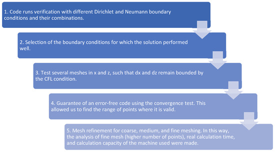
Figure 1.
Optimization algorithm employed.
- Definition of the geological model: defining the geological model that describes the characteristics of the reservoir rock and fluids, as well as their spatial distributions. The model is represented as a three-dimensional mesh of discrete points.
- Definition of the wave model: defining the wave model that describes the propagation of seismic waves in the reservoir. This model is discretized using the finite difference method to obtain a discretized wave equation.
- Definition of boundary conditions: defining the boundary conditions that limit the simulation domain. These conditions include reflection conditions, absorption conditions, and other relevant boundary conditions.
- Source signal generation: generating a source signal representing the seismic energy source used to excite seismic waves in the reservoir.
- Definition of simulation parameters: specifying simulation parameters, such as mesh size, simulation duration, sampling frequency, and source signal parameters.
- Simulation initialization: initializing pressure and velocity values at each grid point to zero at the initial time.
- Simulation iteration: performing simulation iterations using the finite difference method. The discretized wave equation updates the pressure and velocity values at each mesh point during each iteration, while boundary conditions limit the simulation domain.
- Solution evaluation: evaluating the simulation solution against the objectives of petroleum exploration. This evaluation may involve visualizing wave patterns, identifying zones of interest in the reservoir, and estimating reservoir properties, such as permeability and porosity.
- Optimization of simulation parameters: optimizing simulation parameters using an optimization algorithm. Parameters that can be optimized include energy source position and orientation, source signal frequency, and mesh parameters.
- Simulation re-run: repeating the simulation with newly optimized parameters. The new solution is evaluated and the optimization process is repeated iteratively until the desired objective is achieved.
3. Results
Indeed, when simulations involving partial differential equations were performed, apart from the errors of rounding and truncation of the series (remember that the finite difference expressions were derived from a Taylor series development to the second order), there were errors associated with the limitations of adapting the physical model to accurately describe the realistic physical system and the limitations of the boundary conditions. However, convergence and stability tests ensured that the finite difference approximations used in the discretization were correct.
There are ways to calculate the convergence of a code when the analytical solutions are known. For example, by knowing the value of Δx, the minimum number of nodes required to find a numerical solution for Equation (5) could be determined. Furthermore, the Courant–Friedrichs–Lewy (CFL) condition was necessary for converging the numerical solution of partial differential equations in partial derivatives.
To study the stability, it was sufficient that the solutions of the differential equations did not present oscillations (are regular), considering that the solutions depended on time. Let the physical variables p and ρ evolve over a long period of time to verify that they do not present oscillations or jagged peaks. This was performed for a time of 30 s. Figure 2 shows the evolution of the acoustic pressure as a function of time for different meshes Δx. The development remained smooth without showing irregular behaviors during this evolution.
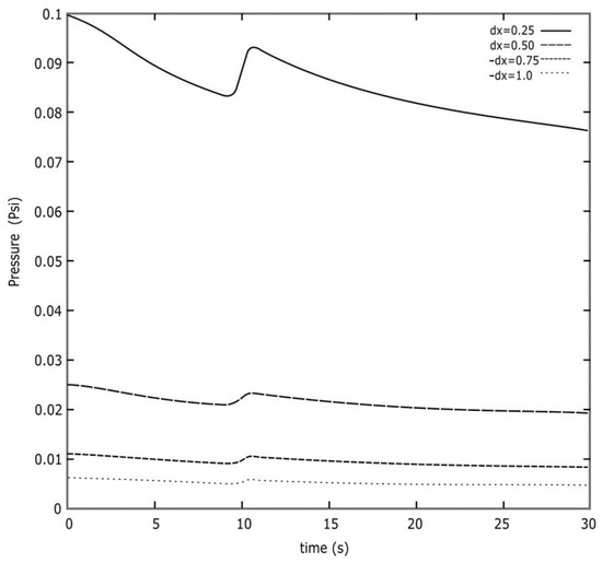
Figure 2.
Acoustic pressure behavior as a function of time for different meshes Δx. The development remains smooth without showing irregular behaviors during the transition.
In Figure 2, the peak observed around 10 s occurs when the wave passes from the first to the second layer. We attempted to mitigate this effect by employing a highly refined mesh (consisting of many points). However, due to the limitations of the machine, some code runs could not effectively smooth out these peaks.
Figure 3 shows the density behavior as a function of distance x for different meshes Δx. The density shows a typical behavior during the simulation for different x values.

Figure 3.
Density behavior as a function of distance x for different meshes Δx. The density shows a typical behavior during the simulation for different values of x and remains smooth without showing irregular behavior.
In some cases, when the analytical solution was not known, one way to perform the convergence was to take as the analytical solution the numerical value of the first iteration of the program and compare it with the numerical value of the second iteration. Then, the value of the second iteration was taken as the analytical solution and compared with the numerical value of the third iteration, and so on.
The convergence consisted of checking how close the numerical solution obtained was to a known analytical solution.
To perform the convergence of the code implemented in Fortran 90, we proceeded as follows: because the finite difference approximation method used in the Taylor series development was of a second order, the error was postulated to also be of the second order in ∆x.
Applying logarithm and its properties to both members of Equation (16):
Equation (16) presented the behavior of a straight slope line equal to two. Plotting Log(error) vs. Log(∆x) presented the error between a known analytical solution and the numerical solution for the acoustic wave equation. A slope approximately equal to two implied that the numerical solution converged with the analytical solution. In this case, a general expression for the convergence calculation, given by the L2 standard, was used for the convergence, provided by:
where fij represents the analytical acoustic pressure derived from the solution of the equation.
where C includes all the constants of Equation (5), and Fij is the numerical solution obtained from the numerical implementation of Equation (10), keeping only the dependence on the z coordinate (14). Making L2 = error, by plotting Log(error) vs. Log(Δx), changing the number of points in x, one has a straight line of slope 1.8, in agreement with the expected second order, as shown in Figure 4.
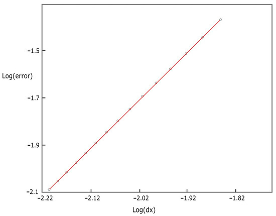
Figure 4.
Convergence for the numerical solution of the wave equation for acoustic pressure. The logarithm of the error, calculated with the L2 standard, is shown with the difference between the numerical and analytical solutions as a function of the logarithm of dx.
Backward and forward finite differences were also implemented in the developed software. In verifying the stability and convergence, it was observed that it was stable only when using centered differences.
A case of particular importance was when time-forward schemes were used as a numerical solution. Consequently, in many simulations, the time step had to be less than a characteristic value. Otherwise, the code may have been unstable and did not yield the correct results. The CFL condition is commonly related to the numerical propagation speed.
For the numerical solution to be stable, the following stability criterion for the standard second-order finite difference scheme for the wave equation is established, as reported in [9,10], and is given by (15):
At each time step, the wavefield propagated at the internal nodes according to Equation (10), and then propagated along the lateral and bottom boundaries employing the difference relations given in [10]. In this work, the relation max (∆x, ∆z) ≤ λ/4 was used, where λ represents the wavelength [11].
3.1. Algorithm
The sources were placed at a particular separation distance called (offset). The sources were assumed to be separated at the same distance to determine the number of shots fired. The integer division between the length of the profile from the location of the initial source (xsource) and the distance between the sources defined the total shots. This is expressed in the following equation:
Once the number of shots was known, they were distributed equally among the number of processors. Thus, the number of shots per processor were obtained from the integer division of the number of shots by the number of processes. The remainder of this division meant one more shot in the first process. In this way, each process generated the locations of its sources and executed the sequential code for each of them.
The authors used a simple geologic model to demonstrate the validity of the code application. The model (Figure 1) comprised three layers. The velocity for the first layer was set at 610 m/s (due to the limitations of the machine used), the second layer at 700 m/s velocity, and the last layer at 830 m/s velocity. Additionally, the authors set a constant density of 2.0 g/cm3 for all three layers.
Figure 5 shows the additional parameters used in the simulation. For this model, it took 98.10 s to place a source on the horizontal reference axis position. Using the data presented in Figure 5, the authors generated 87 horizontally placed sources, resulting in a sequential run time of 98.10 × 87 = 8534.7 s. As the complexity of the model increased and longer recording times were needed, the computational cost also increased.
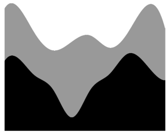
Figure 5.
The geological model was used in the simulation [31]. The depth is displayed, P(m), as a function of distance (m).
This paper demonstrated the validity of the code using a simple geologic model. The model (Figure 5) consisted of three layers. The authors set the velocity of the first layer at 610 m/s (due to limitations in the cluster used), the second layer at 700 m/s, and the last layer at 830 m/s. Additionally, they set a constant density of 2.0 g/cm3 for all three layers. The additional parameters are provided in Table 2.
Table 2.
Parameters considered in the simulation.
For this model, it took 98.10 s to place a source in a horizontal position. Based on the data presented in Figure 2, 87 sources were located horizontally in total. Consequently, firing each source sequentially would result in an execution time of 98.10 × 87 = 8534.7 s, equivalent to over two hours of execution. The computational cost increased if the model was more complex and required a longer recording time.
The code was implemented using a finite difference scheme on a cluster of 16 processors.
Distance (m) 0 2e + 04 4e + 04 6e + 04 8e + 04 10e + 04 P(m) 2.0
Table 2 shows the parameters used in the simulation, including aspects of the receivers’ position and sources.
Figure 6 shows the seismogram generated by propagating the acoustic wave equation on the model of Figure 4 and the parameters presented in Table 2.
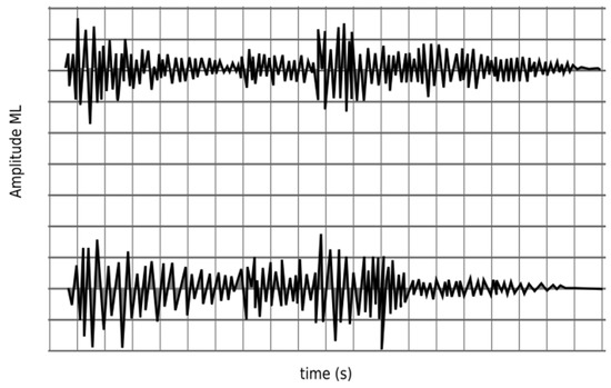
Figure 6.
Simulation seismograms for Nx = N = 10,000 (top) and Nx = N = 15,000 (low).
3.2. Test Dataset Description
During the study, the continuous monitoring of the behavior of the variables involved in the process, such as pressure, wave velocity, amplitude, and travel time, was performed during each iteration cycle to evaluate the behavior of these parameters in the acoustic analysis developed in the oilfield region. This technique allowed the comparison of data obtained in the field with those provided by the mathematical model, to make the appropriate adjustments in the mathematical model that fit the existing boundary conditions in the area of operation. As a result, these adjustments and refinement of the pseudocode allowed us to understand the behaviors of the wave dispersion in different subsurface geological conditions.
The geological conditions in the oil zones influenced the characterization of the geological variables that defined the mathematical model when considering the readings obtained in the measurement process conducted in the field and comparing it with the results obtained using the finite difference approximation method in the seismographic study of wave propagation in the oil zones.
3.3. Information System Architecture
For the development of the research, it was necessary to define a system that allowed globalizing the variables and input data required by the mathematical model in the geological analysis of wave propagation in the oilfields (Figure 7). Furthermore, it was necessary to delimit the domain of the selected region to implement the algorithm for the study of wave propagation in oil exploration. It should be noted that this delimitation allowed us to characterize the geological samples and their behavior in the presence of an oilfield, which constituted a fundamental part in the feeding of the variables of the pseudocode that allowed us to evaluate the behavior of the different geological layers of the subsoil. The system based on the fundamental characteristics of the analytical system of wave propagation in the presence of an incitation disturbance that was propagated in a geological domain was used to evaluate the presence of hydrocarbons in the subsoil.
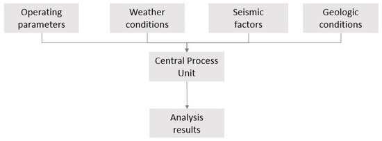
Figure 7.
The operational structure of the developed system.
3.4. Investigation of the Stability of the Generated Results
The researchers observed that the developed pseudocode analyzed and evaluated different oilfield geological samples within the selected domain. The programming simulator proposed in this study was adapted for all the proposed scenarios, producing a satisfactory response that adjusted to the geological behavior in the presence of hydrocarbons in the reservoirs. Notably, they evaluated the stability of the code in a realistic situation using ultrasound equipment for reservoir detection. The simulation software responded consistently to the wave propagation analysis on the oil surface, producing satisfactory results.
To test the stability of the solutions, the researchers subjected the pressure to prolonged durations, considering its time-dependent nature. As the pressure progressed over several units of computational time, its graph exhibited a smooth and consistent pattern throughout this evolution. The absence of unexpected peaks in the pressure graph during the progression was observed and ensured. For maintaining solution stability, calculating the interdependent mesh sizes (dx, dy, dz, and dt) required meticulous consideration to select the appropriate number of points for each mesh. A comprehensive examination of the meshes and spacings in the x, y, z, and t directions was conducted, ensuring their mutual dependence and adherence to the limits imposed by the CFL condition. The paper specified stability conditioned by the CFL condition (refer to Equation (15)), implying a specific relationship that must be fulfilled. Figure 1 illustrates the smooth evolution up to 150 s, with no occurrence of peaks.
3.5. Perspectives and Limitations
Among the study limitations, it can be mentioned that there were many finite difference schemes: backward, forward, and center, among others. The developed code was not stable for all of them. There were, in fact, previous studies where, according to the differential equation under study, it was determined that it was not stable for all cases. The scheme used in this paper was stable for several tests with fine meshes as far as it was possible using the available computers. The boundary conditions that made the code steady were the Dirichlet conditions.
4. Conclusions
According to the wave obtained in the seismogram, the experts determined whether there was oil in the subsoil. The algorithm presented in this paper showed a high efficiency when propagating the acoustic wave equation in a geological profile using a firing line. This algorithm can be used in real seismic exploration studies to refine the acquisition parameters in prospective studies.
The results allow us to conclude that, in a reasonable time, a set of experiments helps decision making regarding recording time, the separation of receivers, the separation of sources, and the maximum frequency range of the source for reliable oil exploration studies.
This algorithm can be used in real seismic exploration surveys to fine-tune acquisition parameters in the prospective surveys.
Different simulations were performed using different parameters, boundary conditions, and meshes. There are solutions better than the finite forward and backward differences for thick meshes with spatial discretizations. When the passage of time is considerably long, the answers are similar and deviate from the analytical solution. For depths greater than 17,400 ft, the code becomes unstable. More accurate results can be obtained using a cluster with more processors.
In the future research conducted in this field, improvements in computational efficiency should be implemented to explore the techniques to improve the computational efficiency of the finite difference simulation method. This study could investigate alternative numbering schemes, optimize code implementations, and use parallel computing techniques to reduce simulation times. In addition, a sensitivity analysis should be performed to assess the impact of various parameters on the simulation results. This research could involve studying the influence of factors, such as mesh size, time step, source frequency, and geological properties, on the accuracy and stability of the simulation.
Author Contributions
Conceptualization, F.S.-C. and L.R.-R.; methodology, F.S.-C.; software, L.R.-R.; validation, F.S.-C., L.R.-R. and J.S.; formal analysis, H.-F.M.-C.; investigation, H.E.V.-L. and O.F.-U.; writing—original draft preparation, F.S.-C. and P.A.-V.; writing—review and editing, F.S.-C. and P.A.-V. All authors have read and agreed to the published version of the manuscript.
Funding
The APC was funded by Universidad de las Américas, Quito, Ecuador.
Institutional Review Board Statement
Not applicable.
Informed Consent Statement
Not applicable.
Conflicts of Interest
The authors declare no conflict of interest.
References
- Clapp, F.G. Review of Present Knowledge Regarding the Petroleum Resources of South America. Trans. AIME 1917, 57, 914–967. [Google Scholar] [CrossRef]
- Herrera-Franco, G.; Montalván, F.J.; Velastegui-Montoya, A.; Caicedo-Potosí, J. Vulnerability in a Populated Coastal Zone and Its Influence by Oil Wells in Santa Elena, Ecuador. Resources 2022, 11, 70. [Google Scholar] [CrossRef]
- Maddela, N.R.; Scalvenzi, L.; Venkateswarlu, K. Microbial degradation of total petroleum hydrocarbons in crude oil: A field-scale study at the low-land rainforest of Ecuador. Environ. Technol. 2016, 38, 2543–2550. [Google Scholar] [CrossRef] [PubMed]
- Lukawski, M.Z.; Anderson, B.J.; Augustine, C.; Capuano, L.E.; Beckers, K.F.; Livesay, B.; Tester, J.W. Cost analysis of oil, gas, and geothermal well drilling. J. Pet. Sci. Eng. 2014, 118, 1–14. [Google Scholar] [CrossRef]
- Assaad, F.A. Surface Geophysical Petroleum Exploration Methods. In Field Methods for Petroleum Geologists; Springer: Berlin/Heidelberg, Germany, 2009; pp. 21–23. [Google Scholar] [CrossRef]
- Dai, N.; Vafidis, A.; Kanasewich, E.R. Wave propagation in heterogeneous, porous media: A velocity-stress, finite-difference method. Geophysics 1995, 60, 327–340. [Google Scholar] [CrossRef]
- Ramırez, J.L.; Larrazabal, G. Imagenología sísmica 3D post-apilamiento en exploración petrolera. In Proceedings of the Conference CIMENICS 2010, Mérida, Venezuela, 22–24 March 2010. [Google Scholar]
- Wang, Y.; Yang, H. Numerical simulation of elastic wave propagation in azimuthally anisotropic media using multi-level finite difference method. Qinghua Daxue Xuebao/J. Tsinghua Univ. 2006, 46, 293–296. [Google Scholar]
- Sabino, T.L.; Brandão, D.; Zamith, M.; Clua, E.; Montenegro, A.; Kischinhevsky, M.; Bulcão, A. Implementation Aspects of the 3D Wave Propagation in Semi-Infinite Domains Using the Finite Difference Method on a GPU Based Cluster; Lecture Notes in Computer Science (Including Subseries Lecture Notes in Artificial Intelligence and Lecture Notes in Bioinformatics); Springer: Berlin/Heidelberg, Germany, 2014; Volume 8584, pp. 426–439. [Google Scholar]
- Bliyeva, D.; Baigereyev, D.; Imomnazarov, K. Computer Simulation of the Seismic Wave Propagation in Poroelastic Medium. Symmetry 2022, 14, 1516. [Google Scholar] [CrossRef]
- Ma, C.; Gao, Y.; Lu, C. Numerical modeling of elastic wave in frequency-domain by using staggered grid fourth-order finite-difference scheme. Adv. Geo-Energy Res. 2019, 3, 410–423. [Google Scholar] [CrossRef]
- Liu, Y.; Guan, Z.; Li, Z.; Wang, Q. Experimental Study on Acoustic Propagation Characteristics in Drill-String. In Proceedings of the International Conference on Computational Intelligence and Communication Networks, Jabalpur, India, 12–14 December 2015. [Google Scholar]
- Huang, H.; LI, Q.; Liu, X.; Yanchao, W.; Liu, C. Low-level faults characteristics of the seismic wave field. Prog. Geophys. 2014, 29, 1298–1305. [Google Scholar]
- Kakavas-Papaniaros, P.A.; Kakavas, M. Stress Wave Interactions in Cracked Rocks for the Investigation of Oil Extraction. 2018. Available online: https://www.researchgate.net/publication/344378990 (accessed on 14 July 2023).
- Peng, M.; Wang, D.; Liu, L.; Liu, C.; Cuican, L. Intelligent recognition of layered geological body based on machine learning and seismic exploration. J. Eng. Geol. 2020, 28, 230–236. [Google Scholar]
- Borregales, M.; Jiménez, O.; Buitrago, S. Generación de mallas de cuadriláteros para yacimientos bidimensionales con fronteras internas complejas. In Proceedings of the VI Encuentro Colombia Venezuela de Estadística, Valencia, Venezuela, 25–29 October 2009. [Google Scholar] [CrossRef]
- Quintero, N.; Calvete, F. Desarrollo de un Modelo Computacional para Flujo Bifásico en tres Dimensiones Usando el Método de Volúmenes Finitos. 2017. Available online: earthdoc.org (accessed on 17 February 2023).
- Perira, J. Simulación computacional en la industria del gas y petróleo. Casos de aplicación. Atenea 2022, 9, 8–10. [Google Scholar]
- Dávila, V. Análisis y Simulación Numérica por MEF de los Esfuerzos y Deformaciones Sometidas a Cargas y Temperaturas en Ductos Terrestres para Transporte de Petróleo; Instituto Politécnico Nacional: Bogotá, Colombia, 2015. [Google Scholar]
- Martínez, M.; Insausti, D.; Corales, A. Análisis y Modelado de los Esfuerzos en una Sección de Cemento de un Pozo Petrolero Utilizando el Método de Elementos de Contorno (MEC). Mec. Comput. 2012, XXXI, 1065–1083. [Google Scholar]
- García, F.; Alarcón, E. Simulación numérica por el Método de los Elementos de Contorno. Utilización de elementos isoparamétricos parabólicos. In Proceedings of the de 1er. Simposium Nacional sobre Modelado y Simulación en la Industria y Servicios Públicos, Sevilla, Spain, 7–9 May 1980. [Google Scholar]
- Del Toro, Y.; Ortiz, J.; Pimienta, Y. Biblioteca Digital Personalizada sobre Simulación Numérica en la Industria Petrolera; Universidad de las Ciencias Informáticas: Havana, Cuba, 2010. [Google Scholar]
- Gao, K.; Fu, S.; Gibson, R.L.; Chung, E.T.; Efendiev, Y. Generalized Multiscale Finite-Element Method (GMsFEM) for elastic wave propagation in heterogeneous, anisotropic media. J. Comput. Phys. 2015, 295, 161–188. [Google Scholar] [CrossRef]
- Marcondes, F.; Sepehrnoori, K. An element-based finite-volume method approach for heterogeneous and anisotropic compositional reservoir simulation. J. Pet. Sci. Eng. 2010, 73, 99–106. [Google Scholar] [CrossRef]
- Blondel, P. Computer-assisted interpretation. In The Handbook of Sidescan Sonar; Praxis Publishing: Chichester, UK, 2009; pp. 249–276. [Google Scholar] [CrossRef]
- Noack, M.M.; Clark, S. Acoustic wave and eikonal equations in a transformed metric space for various types of anisotropy. Heliyon 2017, 3, e00260. [Google Scholar] [CrossRef] [PubMed]
- Mellor, J. The Dirac Delta Function. Medium, 25 de Abril de 2022. Available online: https://www.cantorsparadise.com/the-road-to-quantum-mechanics-part-7-the-dirac-delta-function-374540fae66e (accessed on 16 July 2023).
- Brandão, D.; Zamith, M.; Clua, E.; Montenegro, A.; Bulcão, A.; Madeira, D.; Kischinhevsky, M.; Leal-Toledo, R.C. Performance Evaluation of Optimized Implementations of Finite Difference Method for Wave Propagation Problems on GPU Architecture. In Proceedings of the 22nd International Symposium on Computer Architecture and High-Performance Computing Workshops, Petropolis, Brazil, 27–30 October 2010. [Google Scholar]
- Eftekhari, S. A note on mathematical treatment of the Dirac-delta function in the differential quadrature bending and forced vibration analysis of beams and rectangular plates subjected to concentrated loads. Appl. Math. Model. 2015, 39, 6223–6242. [Google Scholar] [CrossRef]
- De Basabe, J.D.; Sen, M.K. A comparison of finite-difference and spectral-element methods for elastic wave propagation in media with a fluid-solid interface. Geophys. J. Int. 2014, 200, 278–298. [Google Scholar] [CrossRef]
- Xiong, F.; Ba, J.; Gei, D.; Carcione, J. Data-Driven Design of Wave-Propagation Models for Shale-Oil Reservoirs Based on Machine Learning. JGR Solid Earth 2021, 126, e2021JB022665. [Google Scholar] [CrossRef]
- Serpa, M.S.; Cruz, E.H.; Diener, M.; Krause, A.M.; Farrés, A.; Rosas, C.; Panetta, J.; Hanzich, M.; Navaux, P. Strategies to Improve the Performance of a Geophysics Model for Different Manycore Systems. In Proceedings of the International Symposium on Computer Architecture and High-Performance Computing Workshops (SBAC-PADW), Campinas, Brazil, 17–20 October 2017. [Google Scholar]
- Basir, H.M.; Javaherian, A.; Shomali, Z.H.; Firouz-Abadi, R.D.; Gholamy, S.A. Acoustic wave propagation simulation by reduced order modelling. Explor. Geophys. 2018, 49, 386–397. [Google Scholar] [CrossRef]
- Hanindhito, B.; Gourounas, D.; Fathi, A.; Trenev, D.; Gerstlauer, A.; John, L.K. GAPS: GPU-acceleration of PDE solvers for wave simulation. In Proceedings of the International Conference on Supercomputing, Virtual Event, 28–30 June 2022; Volume 2022, pp. 1–13. [Google Scholar]
- Talebitooti, R.; Zarastvand, M.R. The effect of nature of porous material on diffuse field acoustic transmission of the sandwich aerospace composite doubly curved shell. Aerosp. Sci. Technol. 2018, 78, 157–170. [Google Scholar] [CrossRef]
- Wang, M.; Xu, S. Finite-difference time dispersion transforms for wave propagation. Geophysics 2015, 80, WD19–WD25. [Google Scholar] [CrossRef]


Disclaimer/Publisher’s Note: The statements, opinions and data contained in all publications are solely those of the individual author(s) and contributor(s) and not of MDPI and/or the editor(s). MDPI and/or the editor(s) disclaim responsibility for any injury to people or property resulting from any ideas, methods, instructions or products referred to in the content. |
© 2023 by the authors. Licensee MDPI, Basel, Switzerland. This article is an open access article distributed under the terms and conditions of the Creative Commons Attribution (CC BY) license (https://creativecommons.org/licenses/by/4.0/).