Dynamic Weight and Mapping Mutation Operation-Based Salp Swarm Algorithm for Global Optimization

Abstract

The salp swarm algorithm imitates the swarm behavior of salps during navigation and hunting that has been proven the superiority of search for best solution. However, although it has sufficient global search ability, it is still worth paying attention to problems of falling into local optima and lower convergence accuracy. This paper proposes some improvements to the salp swarm algorithm that are based on a nonlinear dynamic weight and the mapping mutation operation. Firstly, the nonlinear dynamic weight is helpful for further optimizing the transition from exploration to exploitation and alleviating the local optima stagnation phenomena. Secondly, utilizing a mapping mutation operation can increase the diversity of followers in algorithm, to avoid getting trapped into the local optima during the search and provide a better optimal solution. The proposed algorithm is characterized by a stronger global optimization capability and high convergence accuracy. Finally, to confirm the effectiveness of the proposed algorithm, comparative experiments based on other well-known swarm-based algorithms and each improvement for the original algorithm are conducted. The quantitative results and convergence curves among several algorithms demonstrate that the enhanced algorithm with the nonlinear dynamic weight and mapping mutation operation can outperform the original algorithm.

1. Introduction

Recently, metaheuristic optimization algorithms have surprisingly attracted the attention of many researchers due to the flexibility, nongradient mechanism, and ability to avoid local optima. Inspired by bionics and random phenomena in nature, these algorithms are optimization algorithms that combine random algorithms with other algorithms. According to different heuristic mechanisms, meta-heuristic optimization algorithms mainly categorize into two categories: evolutionary algorithms [1] and swarm optimization algorithms [2]. On the one hand, the evolutionary algorithms are based on biological evolutionary behaviors, and the evolutionary algorithm that is famous for imitating the concept of Darwinian theory of evolution is the genetic algorithm (GA) [3]. In addition, differential evolution (DE) [4], which uses crossover, mutation, and reproduction in genetics to design the genetic operations, is also a representative algorithm of these.

Otherwise, swarm-based optimization algorithms are proposed by mimicking the swarms and animals’ social behaviors. Among swarm optimization algorithms, either particle swarm optimization (PSO) [5] or ant colony optimization (ACO) [6] are the most representative. PSO imitates the collective social behavior of birds during flight and hunting, while ACO is proposed by imitating the social group behavior of ant colonies during the foraging process. There are some classic algorithms based on swarm intelligence optimization technology, for instance, dolphin echolocation (DEL) [7,8], firefly algorithm (FA) [9,10], and bat algorithm (BA) [11]. Furthermore, FA mimics the mating behavior of fireflies in nature, while DEL and BA simulate dolphins and navigating bats, respectively. Moreover, some latest developed and effective algorithms are electric fish optimization (EFO) [12], which simulates the predation and communication behaviors of electric fish, whale optimization algorithm (WOA) [13], which imitates the hunting process of humpback whales, and antlion optimizer (ALO) [14], which simulates the foraging of antlions in nature.

In 2017, Mirjalili released the salp swarm algorithm (SSA) [15], which mimics the salp swarm. Recently, SSA has received extensive attention from researchers in many fields, including the feature selection for image classification [16], the variable speed wind generators [17], and engineering optimization problems [18]. SSA mainly imitates the swarm behaviors of salp chains navigating and foraging in the ocean. The categories of salp chains are leaders and followers. Generally, leaders play the role of leading the salp chains in the swarm, and at the same time, leaders move towards the food source. Followers are guided by the leaders through their chained bahaviors to move. The salp chains utilize the interactive behavior of leaders and followers to prey quickly and accurately in the ocean space. To alleviate the local optimum stagnation and promote convergence accuracy, Zhang et al. [19] introduced the adaptive control parameter, and the best gray wolf algorithm dominates the position update stage of followers and the last stage of the population, respectively. The improved SSA enhances the local exploitative performance of the followers and helps the population search for the target faster. To solve the phenomena of local stagnation, Duan et al. [18] utilized chaotic initialization tactics and meristic accommodative population. In addition, a simulated annealing mechanism ground on meristic disturbance is utilized to improve the competence to escape from the local optimum. Zhuo et al. [20] primarily engineered an update mechanism for leaders over logistic mapping to boost the diversity of the population and exploited a dynamic learning dependent follower renewal mechanism to strengthen the global search capability of the algorithm. Hussien et al. [21] proposed a novel SSA called OBSSA, which relies on an opposition-based learning strategy to improve the capacity to circumvent local optima. The algorithm consists of two phases: in the first phase, OBL is used to augment the initialized population; in the second phase, OBL is applied to the population update process in each iteration. Ibrahim et al. [22] proposed a new algorithm named SSAPSO by mixing PSO with SSA, which enhanced the exploration and utilization efficiency of the algorithm. The base construction of the SSA algorithm is altered with the improvement of the update stage of the population location. This revision incorporates the update regime of PSO into the main construction of SSA. This consolidation creates more flexibility for SSA in exploring populations, ensuring that populations are diverse and can attain optimal values rapidly.

In light of the No Free Lunch (NFL) theorem [23,24], no algorithm can settle all optimization problems. Similar to other swarm optimization algorithms, SSA has local optima stagnation phenomena and low convergence accuracy. Although many researchers have made many improvements to the classic SSA, SSA can still be improved to enhance its ability to moderate the local optima stagnation and convergence accuracy. Therefore, this paper uses some improvements to boost the global search capacity and alleviate premature convergence.

In response to the above-mentioned problems suffered by traditional SSA, this presented paper proposes two methods for leaders and followers. First, the application of the nonlinear dynamic weight strategy to further optimize the transfer control parameter in leaders. In the optimization algorithms based on meta-heuristics, there are two key tasks, called exploration and exploitation [25,26]. In the exploration task, SSA uses the leaders’ behavior toward food sources to find the best areas. In the exploitation task, however, followers use their own information interaction and the leaders’ guidance to realize the behavior of searching for the first-rank solution in the most promising area. Traditional SSA uses nonlinear control strategy to achieve the transition from global exploration to local exploitation, and good results have been obtained. In this paper, a nonlinear control parameter, namely dynamic weight, is used to fine-tune the transfer control parameter to achieve the secondary control of the transition. Second, in order to increase the dimensionality of the followers during the position update and to avoid getting trapped into the local optima, a mapping mutation operation is introduced. When followers find that they cannot search for a better position during the search process, the mapping mutation operation can keep the algorithm from getting trapped into the local optima by providing a random jump. By implementing these two improvements to the traditional SSA, the improved SSA named WMSSA can more smoothly transfer from global exploration to local exploitation, and can make full use of the advantages brought by the mapping mutation operation, which can expand the population variety of followers and promote the algorithm to escape local optima. Finally, to validate the performance of the improved SSA, some comparative experiments based on several effective and classical swarm optimization algorithms and 10 benchmark functions are implemented. The statistics show that proposed WMSSA outperforms classical SSA and other swarm-based optimization algorithms.

This article is divided into sections. Section 2 shows the classical SSA and its literature review. The detailed mathematical type of the modified SSA is presented in Section 3. To assess the overall effectiveness of the modified SSA, various kinds of simulation experiments and analysis that compare the improved SSA with other four celebrated swarm-based optimization algorithms (containing the classical SSA) and compare classical SSA with the corresponding algorithms for each improvement are provided in Section 4. Section 5 shows the final conclusion and the future research direction.

2. Salp Swarm Algorithm

SSA is proposed by simulating the swarming behaviors of salps in the deep sea. In the living environment of salps, in order to achieve better movement and foraging through fast coordinated changes, salps usually form a chain-like special swarming behavior. Therefore, to mimic the chain behavior of salps, the population of SSA consists of two classes: leaders and followers. The leaders are led by the food source and guide the followers to move.

2.1. The Initialization of Population

Here, the population of salps is expressed as an N × D-dimensional matrix called $X_{N,D}$, as shown in Equation (1). In addition, suppose that there is a prey named F, used as the target of the optimization problem. Then, the population of SSA is randomly initialized to Equation (2):

$$X_{N,D}=\left[\begin{array}{cccc}{x}_{1,1}& x_{1,2}& \cdots & x_{1,D}\\ x_{2,1}& x_{2,2}& \cdots & x_{2,D}\\ ⋮& ⋮& \ddots & ⋮\\ x_{N,1}& x_{N,2}& \cdots & x_{N,D}\end{array}\right]$$

(1)

$$X_{N,D}=rand(N,D)\times (ub-lb)+lb$$

(2)

where $X_{N,D}$ contains the population information of N salps with dimension D, $rand(N,D)$ represents a N × D-dimensional matrix created by using a random function, $ub$ indicates the upper bound of the search space, and $lb$ indicates the lower bound of the search space.

2.2. The Position Update of Leaders

Salps form a chain-like structure and leaders are guided by the food source $F={[F_1,F_2,\cdots ,F_D]}^T$ to update their position adaptively. The position of leader equation is shown below:

$$X_{i,j}=\left\{\begin{array}{cc}{F}_j+c_1((u{b}_j-l{b}_j)c_2+l{b}_j),\hfill & c_3\ge 0.5\hfill \\ F_j-c_1((u{b}_j-l{b}_j)c_2+l{b}_j),\hfill & c_3<0.5\hfill \end{array}\right.$$

(3)

where $i=1,2,\cdots ,N/2$, $j=1,2,\cdots ,D$, and $X_{i,j}$ denotes the position of the i-th salp of leaders in the j-th dimension. Moreover, leaders are the top $N/2$ salps according to the objective function value. $F_j$ is the location of the prey in the j-th dimension. The random numbers $c_2$ and $c_3$ are evenly distributed within the boundary of [0, 1] at each iteration, and they control the step size and the next direction, respectively, for leaders.

Formula (3) shows that the leader’s position update is only related to the location of the food. In this paper, $c_1$ is the convergence factor in the optimization algorithm, which plays a role in balancing global exploration and local development, $c_1$ is a value that gradually decreases with the iteration of the algorithm (dynamic update step) and $c_1$ is a 2-0 decreasing function, l represents the current iteration number, and $l_{max}$ represents the maximum iteration number. The mathematical expression can be expressed as:

$$c_1=a\times e^{-{\left(\frac{b\times l}{l_{max}}\right)}^2}$$

(4)

where l represents the present iteration number and $l_{max}$ is the maximal iteration number. In SSA, a and b are invariables ($a=2$ and $b=4$).

2.3. The Position Update of Followers

In the process of moving and hunting, followers move sequentially in a chain without random movement. On the basis of Newton’s law, therefore, the equation for updating the location is utilized to indicate the movement distance of the follower:

$$S=\frac{1}{2}a{t}^2+v_{0}t$$

(5)

where S denotes the movement distance, t is time, $v_0$ is the original velocity, and a represents the acceleration of movement. For an optimization problem, $t=1$, $v_0=0$ and $a=\frac{v-v_0}{t}$ in each iteration. In addition, because the follower moves closely following the previous salp, the speed $v=\frac{X_{i-1,j}^l-X_{i,j}^l}{t}$. Then, Equation (5) can be expressed as:

$$S=\frac{1}{2}(X_{i-1,j}^l-X_{i,j}^l)$$

(6)

According to the above explanation, the followers’ location update formula is as follows:

$$X_{i,j}^{l+1}=X_{i,j}^l+S=\frac{1}{2}(X_{i,j}^l+X_{i-1,j}^l)$$

(7)

where $i>N/2$, $X_{i,j}^{l+1}$ and $X_{i,j}^l$ are the positions of the i-th salp of followers in the j-th space at iteration $(l+1)$ and l, respectively. The flow diagram of the original SSA is presented in Figure 1.

As shown in Figure 1, the classic SSA can be improved in the following aspects, such as the population initialization stage, the control parameter $c_1$, the position update formula of leaders, the position update formula of followers, and the last stage of the population. In order to ease to fall into local optimum and low convergence accuracy, Zhao et al. [23] introduced the adaptive control parameter and the elite gray wolf domination strategy into the position update stage of followers.

3. Improved Salp Swarm Algorithm

Although, the SSA can accomplish a smooth balance among the exploration and exploitation, it still causes the algorithm to premature convergence and reduce the quality of the optimal solution due to the lack of diversity of followers. Furthermore, facing the improved SSA, the transition parameter used in the classic SSA need to be fine-tuned to adapt to better algorithm performance. Meanwhile, to enhance further the performance of the algorithm, a dynamic weight is introduced to more accurately control the transition parameter. Therefore, the following developments are utilized to improve its performance, according to an in-depth study of the SSA.

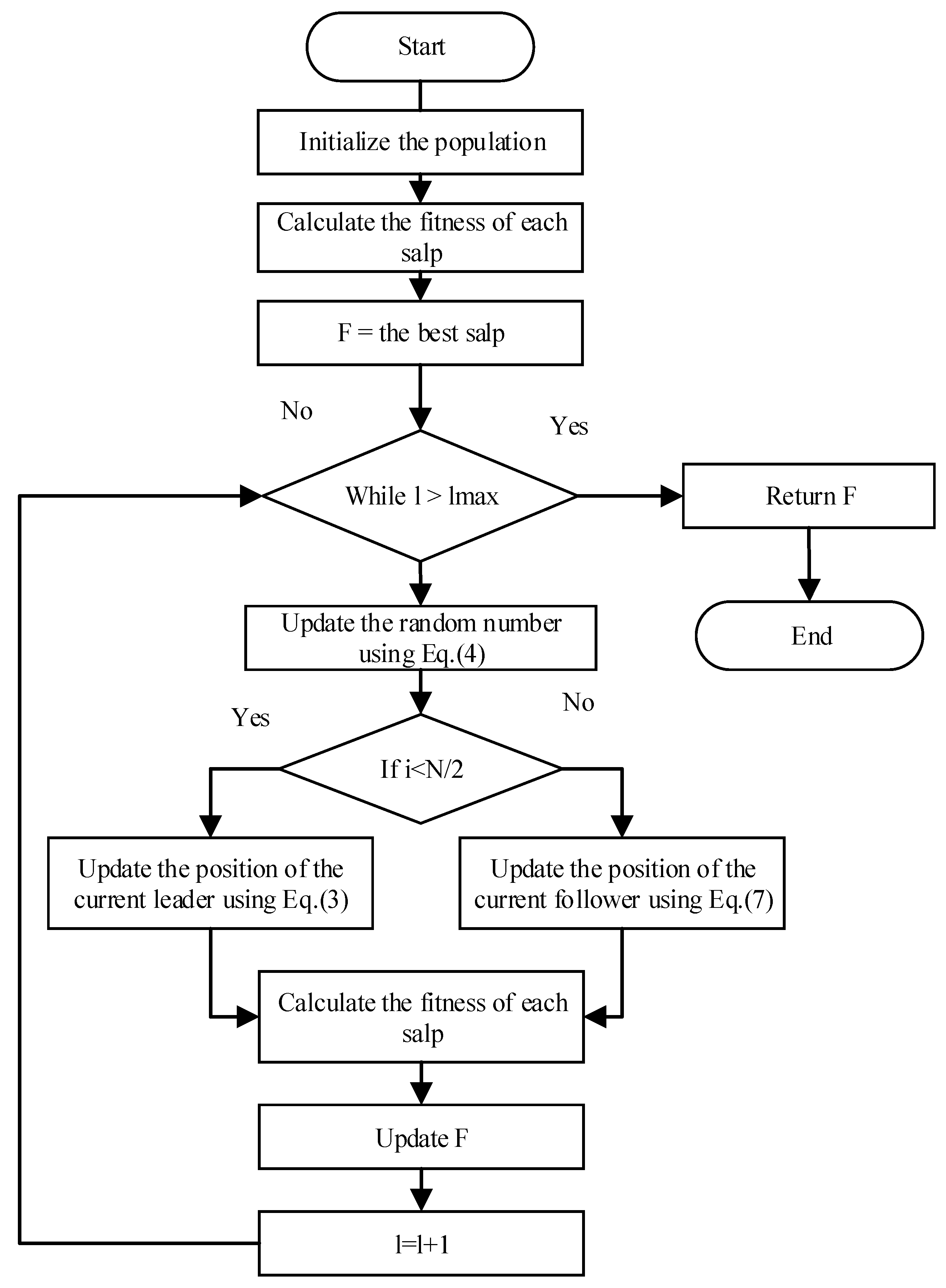
As shown in Figure 1, after updating all members of the population in the leader and follower stages of the SSA algorithm, the algorithm iteration is completed, and the new values, objective functions, and the best proposed solutions of the population members are determined. The algorithm then proceeds to the next iteration and continues to update the population members according to Formulas (3) through (7) until the last iteration of the algorithm is reached. After the SSA is fully implemented, the best proposed solution obtained during the algorithm iteration is taken as the quasi-optimal solution for the given optimization problem.

3.1. The Mapping Mutation Operation for Followers

As shown in the SSA, followers use Equation (7) to update their current position, which shows a classic movement ground on the Newton’s law. However, this kind of movement also leads to the single movement of followers and low population diversity. Therefore, a mapping mutation operation, which is adopted in the improved SSA called MOSSA, is given by:

$$X_{i,j}^{l+1}=\left\{\begin{array}{cc}{X}_{i,j}^l\times (1+G\left(\beta \right)),\hfill & c_4\ge 0.5\hfill \\ l{b}_j+\beta \times (u{b}_j-l{b}_j),\hfill & c_4<0.5\hfill \end{array}\right.$$

(8)

where $c_4$ is a stochastic number from the boundary [0, 1], Suppose the probability density of continuous random variable $\beta$ is $G\left(\beta \right)$, and it can be seen from the characteristics of normal distribution that Gaussian variation is also focused on searching a local region near the original individual. Formula (8) $G\left(\beta \right)$ is a Gaussian mutation operation [27] and $\beta$ is a stochastic number produced by the Tent chaotic map [28].

In the MOSSA, the density function of the normal distribution, which is utilized to advance the variety of followers during the search course, is shown as follows:

$$G\left(\beta \right)=\frac{1}{\sigma \sqrt{2\pi }}{e}^{-\frac{{(\beta -\mu )}^2}{2{\sigma }^2}}$$

(9)

where $\mu$ ($\mu$ = 0) is a mean and ${\sigma }^2$ (${\sigma }^2$ = 1) is the variance of candidate measure. Hence, the Gaussian mutation operation used to obtain a new position of follower is calculated as follows:

$$X_{i,j}^{l+1}=X_{i,j}^l\times (1+G\left(\beta \right))$$

(10)

Due to the traversal and nonrepeatability of the chaos, it can achieve a more effective search process than the random search. Thus, MOSSA uses the Tent chaotic mapping to generate a stochastic number, which can boost the search capacity of the algorithm. The particular expression is as follows:

$${\beta }_{k+1}=c_5\times {\beta }_k\times (1-{\beta }_k)$$

(11)

where $c_5$ is control parameter (default = 4) [26]. Figure 2 shows the random number distribution generated by Tent Chaos after 200 iterations. In the optimization algorithm, the more evenly the initialized population is distributed in the search space, the more beneficial it is to improve the optimization efficiency and solving accuracy of the algorithm. The chaotic sequence generated by Tent mapping has the following advantages.

• Strong randomness: Tent chaos has a high degree of randomness and unpredictability, and can generate sequences with good randomness. This randomness can help the swarm intelligence algorithm to better explore the solution space in the search process and avoid falling into the local optimal solution.
• Wide area search ability: Tent Chaos has a wide area search ability, which can carry out more uniform and comprehensive search in the solution space. This helps the swarm intelligence algorithm to fully explore the solution space in the search process and improve the global search ability of the algorithm.
• Easy to implement and calculate: The calculation of Tent Chaos is simple, as only a simple mathematical operation is required. This makes Tent Chaos easy to implement and calculate, and can be easily integrated into swarm intelligence algorithms.
• Adjustability: The Tent Chaos function has one parameter, the chaos control parameter. By adjusting this parameter, you can adjust the degree of chaos and random property of Tent chaos, and then affect the search behavior of the algorithm. This adjustability makes Tent Chaos suitable for different types of optimization problems and algorithmic requirements.

Combining the Gaussian mutation operation and the Tent chaotic map, when followers cannot produce a better solution, the MOSSA can generate a new solution. By making use of the strengths of the chaotic mapping and mutation operation, they promote the search capacity and enhance the diversity of the population for followers.

3.2. A Dynamic Weight for Leaders

There is a control parameter $c_1$ in SSA, which can effectively balance the transition from the global exploration to the local exploitation. Thus, $c_1$ can also be called a transition parameter. Through the observation of Equation (4), the result shows that $c_1$ adopts a nonlinear model, and it adaptively attenuates from the constant 2 to 0 with the increase of iterations. When the transition parameter is greater than 1, the algorithm performs the global exploration to find the desired search area; when it is less than 1, the algorithm starts to exploit the local area to obtain an accurate estimate. However, after the use of the mapping mutation operation for followers, we observed that the transition parameter $c_1$ used in the classic SSA is not too suitable for the algorithm. Therefore, the fine-tuned transition parameter $c_1$ is specifically expressed as:

$$c_1=a\times 3^{-{\left(\frac{b\times l}{l_{max}}\right)}^2}$$

(12)

where a ($default=2$) and b ($default=5$) are constants. Besides, the algorithm that uses the mapping mutation operation and the fine-tuned transition parameter can be called IMOSSA.

Even though SSA has improved, as mentioned above, a lot of problems still require more precise nonlinear changes to avoid the locally optimal solution. Therefore, this paper proposes to use a nonlinear dynamic weight to adaptively control the transition parameter $c_1$, which is inspired by the inertia weight in the particle swarm optimization [29]. The dynamic weight is as follows:

$$\omega ={\omega }_{max}-({\omega }_{max}-{\omega }_{min})\times {\left(\frac{l}{l_{max}}\right)}^{(1/l)}$$

(13)

where ${\omega }_{max}$ and ${\omega }_{min}$ are expressed as the upper bound and lower bound of the dynamic weight $\omega$, respectively. Furthermore, ${\omega }_{max}$ and ${\omega }_{min}$ are constant values (${\omega }_{max}$ = 1, ${\omega }_{min}$ = 0.0001).

Therefore, according to Equations (12) and (13), the improved position update of leaders is defined as:

$$X_{i,j}=\left\{\begin{array}{cc}{F}_j+\omega ·c_1((u{b}_j-l{b}_j)c_2+l{b}_j),\hfill & c_3\ge 0.5\hfill \\ F_j-\omega ·c_1((u{b}_j-l{b}_j)c_2+l{b}_j),\hfill & c_3<0.5\hfill \end{array}\right.$$

(14)

Based on the dynamic weight strategy, the algorithm has a larger dynamic weight at initial stage of the search and increases the global exploration capacity; at a later stage, the dynamic weight is smaller and heightens the local exploitation capacity of the algorithm. By precisely controlling the fine-tuned transition parameter $c_1$ again, the improved algorithm not only improves the transition effect from the exploration to exploitation, but also accelerates the rate of convergence. The comparison of the fine-tuned transition parameter and the dynamic weight with the original transition parameter $c_1$ is presented in Figure 3.

Equation (12) and Figure 3 show that compared with the original control parameter, the fine-tuned transition parameter still presents a smooth transition from the exploration to exploitation as a whole, but the curve will transfer from the exploration to exploitation at a faster rate of convergence. In addition, according to Equation (13), the attenuation curve in Figure 3 shows that initially, the value of the dynamic weight is high and after a few iterations, its value decreases in a nonlinear tendency to a smaller value. The tendency of nonlinear transition is beneficial to promote the algorithm to transfer from the global exploration to local exploitation. The implementation of the improved algorithm called WMSSA ground on all above proposed tactics is presented in Figure 4.

After adding nonlinear dynamic weights in the exploration phase and mapping variation operations in the development phase of the SSA algorithm, as shown in Figure 4, Formulas (12)–(14) updates the leader and Formulas (7) and (8) updates the follower until the last iteration of the algorithm is reached.

3.3. Complexity Analysis

In this section, the computational complexity of the proposed SSA algorithm is analyzed. The computational complexity initialized by the SSA algorithm is equal to $O\left(N\right)$, where N is the number of population members of SSA. It is known that in SSA, in each iteration, each member of the population is updated in two stages, namely leader and follower, and its objective function is evaluated, after which the computational complexity of the update process is equal to $O\left(2l_{max}\times N\times D\right)$, where Imax is the maximum number of iterations and D is the number of problem variables. Therefore, the computational complexity of the proposed SSA algorithm is equal to $O\left(N\times \left(1+2l_{max}\times D\right)\right)$.

4. Experimental Results and Analysis

To verify the superior effectiveness of the proposed WMSSA, three experiments are conducted.

Experiment 1 is executed to adjust the parameters of the devised algorithm. In the algorithms ground on the swarm optimization, either population size N or maximum number of iterations $l_{max}$ play important roles. Appropriate parameters can not only exert the effectiveness of the algorithm, but promote the execution efficiency of the algorithm.

Experiment 2 contains the estimation of the proposed WMSSA and its contrast with some variants based on the developments of this paper on fixed-dimensional benchmark test issues. The benchmark test, which contain two types, i.e., the unimodal functions and the multimodal functions, was selected from the literature [15]. The mathematical formulas of the issues are outlined in

Table 1. Description of the benchmark test functions.

Function	Dim	Range	${\mathit{f}}_{\mathbf{min}}$
$F1\left(x\right)={\displaystyle \sum _{i=1}^n}{x}_i^2$	30	[−100, 100]	0
$F2\left(x\right)={\displaystyle \sum _{i=1}^n}|x_i|+{\displaystyle \prod _{i=1}^n}|x_i|$	10	[−10, 10]	0
$F3\left(x\right)={\displaystyle \sum _{i=1}^n}{\left({\displaystyle \sum _{j=1}^i}{x}_j\right)}^2$	10	[−100, 100]	0
$F4\left(x\right)=\underset{i}{max}\left\{|x_i|,1\le i\le n\right\}$	10	[−100, 100]	0
$F5\left(x\right)={\displaystyle \sum _{i=1}^n}\left(\right|x_i+0.5{\left|\right)}^2$	10	[−100, 100]	0
$F6\left(x\right)={\displaystyle \sum _{i=1}^n}-x_{i}sin\left(\sqrt{|x_i|}\right)$	10	[−500, 500]	−418.9829 × n
$F7\left(x\right)={\displaystyle \sum _{i=1}^n}[x_i^2-10cos\left(2\pi x_i\right)+10]$	10	[−5.12, 5.12]	0
$F8\left(x\right)=-20exp(-0.2\sqrt{\frac{1}{n}{\displaystyle \sum _{i=1}^n}{x}_i^2})-exp(\frac{1}{n}{\displaystyle \sum _{i=1}^n}cos\left(2\pi x_i\right))$	10	[−32, 32]	0
$+20+e$
$F9\left(x\right)=\frac{\pi }{n}\{10sin\left(\pi y_1\right)+{\displaystyle \sum _{i=1}^{n-1}}{(y_i-1)}^2[1+10{sin}^2\left(\pi y_{i+1}\right)]$	10	[−50, 50]	0
$+{(y_n-1)}^2\}$$+{\displaystyle \sum _{i=1}^n}u(x_i,10,100,4)$
$y_i=1+\frac{x_i+1}{4}$
$u(x_i,a,k,m)=\left\{\begin{array}{cc}k{(x_i-a)}^m\hfill & x_i>a\hfill \\ 0\hfill & -a<x_i<a\hfill \\ k{(-x_i-a)}^m\hfill & x_i<-a\hfill \end{array}\right.$
$F10\left(x\right)=0.1\{{sin}^2\left(3\pi x_1\right)+{\displaystyle \sum _{i=1}^n}{(x_i-1)}^2[1+{sin}^2(3\pi x_i+1)]$	10	[−50, 50]	0
$+{(x_n-1)}^2[1+{sin}^2\left(2\pi x_n\right)]\}+{\displaystyle \sum _{i=1}^n}u(x_i,5,100,4)$

. All test functions between F1 and F5 are unimodal problems and F6–F10 are multimodal problems. The contrast is established on several statistics include standard deviation of the function, maximum, minimum, and mean. To reduce random errors, the data are recorded 30 times.

Experiment 3 details other swarm-based optimization algorithms using the same benchmark test problems and the number of trials as Experiment 1. However, this contrasts the ground on mean, criterion deviation, and convergence behaviors of algorithms. The experimental environment used for Experiment 1, 2, and 3 is presented in

Table 2. The configuration of the experimental computer.

Name	Setting
Hardware
CPU	Intel Core I i5 processor
Frequency	2.5 GHz
RAM	8 GB
Hard drive	1 TB
Operating system	Windows 10
Language	MATLAB R2017b

.

4.1. Experiment 1

In the WMSSA, different parameter values from the population size or the maximum iteration times $l_{max}$ can affect the performance of the algorithm. First, in terms of the parameter $l_{max}$, this section conducts a comparative experiment of 10 test functions based on the minimum and maximum values for different $l_{max}$ values. Furthermore, the experiment is repeated 30 iterations independently to guarantee the robustness of the algorithm results. In Figure 5, since some function-based results are presented in semi-logarithmic coordinates, the zero values corresponding to functions 6 and 7 are not reflected. It can be seen from the minimum value that when the parameter $l_{max}$ is $l_{max}=1000$ and $l_{max}=1500$, the experimental results have similar results, and the results are also better than the case of the parameter $l_{max}=100$ and $l_{max}=500$. In addition, according to the comparison results based on the maximum value, although the maximum values have a slight deviation, when the number of iterations of the swarm optimization algorithm increase, the running speed of the algorithm will be greatly affected under the same convergence accuracy. Therefore, the parameter $l_{max}$ is set to the fixed value $l_{max}=1000$. Second, the parameter N in the algorithm WMSSA is analyzed. The experiment is achieved when N is equal to 10, 30, 50, and 100 separately. Furthermore, it will contrast the convergence results of different population sizes under $l_{max}=1000$. As is shown in Figure 6, the convergence curve can reach the similar optimal value when the population magnitude is set as 50 and 100. Therefore, the parameters $N=30$ and $l_{max}=1000$ are selected.

4.2. Experiment 2

In this subsection, the effectiveness of the WMSSA compared with some changes of the SSA, which are mentioned in this paper for further studying the improvements of each development to the classic SSA. The numerical results, which are evaluated by metaheuristic algorithms on 10 benchmark test problems, can be seen in

Table 3. Comparison of results obtained by the proposed WMSSA and other variants based on classic SSA.

Fun	Algorithm	Max	Min	Mean	Std
F1	SSA	1.70 × 10${}^{-08}$	7.03 × 10${}^{-09}$	1.27 × 10${}^{-08}$	2.49 × 10${}^{-09}$
	MOSSA	2.03 × 10${}^{-08}$	1.07 × 10${}^{-09}$	1.33 × 10${}^{-08}$	4.23 × 10${}^{-09}$
	IMOSSA	2.72 × 10${}^{-17}$	1.47 × 10${}^{-18}$	6.38 × 10${}^{-18}$	6.19 × 10${}^{-18}$
	OBSSA	1.70 × 10${}^{-08}$	5.68 × 10${}^{-09}$	1.14 × 10${}^{-08}$	2.67 × 10${}^{-09}$
	WMSSA	3.96 × 10${}^{-\mathbf{21}}$	4.10 × 10${}^{-\mathbf{26}}$	1.76 × 10${}^{-\mathbf{22}}$	7.22 × 10${}^{-\mathbf{22}}$
F2	SSA	4.90 × 10${}^{-03}$	4.89 × 10${}^{-06}$	1.73 × 10${}^{-04}$	9.00 × 10${}^{-04}$
	MOSSA	1.04 × 10${}^{-05}$	5.00 × 10${}^{-06}$	7.51 × 10${}^{-06}$	1.39 × 10${}^{-06}$
	IMOSSA	1.33 × 10${}^{-07}$	6.52 × 10${}^{-11}$	4.56 × 10${}^{-09}$	2.43 × 10${}^{-08}$
	OBSSA	1.41 × 10${}^{-05}$	3.30 × 10${}^{-06}$	7.45 × 10${}^{-05}$	2.32 × 10${}^{-06}$
	WMSSA	2.89 × 10${}^{-\mathbf{13}}$	6.83 × 10${}^{-\mathbf{15}}$	2.02 × 10${}^{-\mathbf{14}}$	5.09 × 10${}^{-\mathbf{14}}$
F3	SSA	4.60 × 10${}^{-09}$	2.55 × 10${}^{-10}$	2.05 × 10${}^{-09}$	9.87 × 10${}^{-10}$
	MOSSA	3.62 × 10${}^{-09}$	1.05 × 10${}^{-09}$	1.96 × 10${}^{-09}$	6.00 × 10${}^{-10}$
	IMOSSA	2.87 × 10${}^{-15}$	2.08 × 10${}^{-19}$	1.18 × 10${}^{-16}$	5.23 × 10${}^{-16}$
	OBSSA	3.76 × 10${}^{-09}$	7.22 × 10${}^{-10}$	1.89 × 10${}^{-09}$	9.10 × 10${}^{-10}$
	WMSSA	7.60 × 10${}^{-\mathbf{20}}$	8.29 × 10${}^{-\mathbf{27}}$	5.27 × 10${}^{-\mathbf{21}}$	1.62 × 10${}^{-\mathbf{20}}$
F4	SSA	2.34 × 10${}^{-05}$	8.07 × 10${}^{-06}$	1.58 × 10${}^{-05}$	3.69 × 10${}^{-06}$
	MOSSA	2.30 × 10${}^{-05}$	5.27 × 10${}^{-06}$	1.66 × 10${}^{-05}$	4.14 × 10${}^{-06}$
	IMOSSA	3.22 × 10${}^{-10}$	1.02 × 10${}^{-10}$	2.02 × 10${}^{-10}$	5.33 × 10${}^{-11}$
	OBSSA	2.07 × 10${}^{-05}$	6.83 × 10${}^{-06}$	1.49 × 10${}^{-05}$	3.23 × 10${}^{-06}$
	WMSSA	3.60 × 10${}^{-\mathbf{14}}$	1.15 × 10${}^{-\mathbf{14}}$	2.22 × 10${}^{-\mathbf{14}}$	5.96 × 10${}^{-\mathbf{15}}$
F5	SSA	1.11 × 10${}^{-09}$	1.57 × 10${}^{-10}$	5.17 × 10${}^{-10}$	2.08 × 10${}^{-10}$
	MOSSA	1.41 × 10${}^{-09}$	3.38 × 10${}^{-10}$	8.51 × 10${}^{-10}$	2.55 × 10${}^{-10}$
	IMOSSA	1.99 × 10${}^{-19}$	4.80 × 10${}^{-20}$	1.09 × 10${}^{-19}$	3.66 × 10${}^{-20}$
	OBSSA	1.00 × 10${}^{-09}$	3.04 × 10${}^{-10}$	6.09 × 10${}^{-10}$	1.65 × 10${}^{-10}$
	WMSSA	2.17 × 10${}^{-\mathbf{27}}$	3.22 × 10${}^{-\mathbf{28}}$	1.22 × 10${}^{-\mathbf{27}}$	4.31 × 10${}^{-\mathbf{28}}$
F6	SSA	−2.21 × 10${}^{+03}$	−3.42 × 10${}^{+03}$	−2.78 × 10${}^{+03}$	3.51 × 10${}^{+02}$
	MOSSA	−4.19 × 10${}^{+\mathbf{03}}$	−4.19 × 10${}^{+03}$	−4.19 × 10${}^{+03}$	7.58 × 10${}^{-10}$
	IMOSSA	−4.19 × 10${}^{+\mathbf{03}}$	−4.19 × 10${}^{+03}$	−4.19 × 10${}^{+03}$	2.01 × 10${}^{-12}$
	OBSSA	−2.39 × 10${}^{+03}$	−3.59 × 10${}^{+03}$	−2.81 × 10${}^{+03}$	2.82 × 10${}^{+02}$
	WMSSA	−4.19 × 10${}^{+\mathbf{03}}$	−4.19 × 10${}^{+\mathbf{03}}$	−4.19 × 10${}^{+\mathbf{03}}$	1.95 × 10${}^{-\mathbf{12}}$
F7	SSA	2.89 × 10${}^{+01}$	4.97 × 10${}^{+00}$	1.66 × 10${}^{+01}$	6.19 × 10${}^{+00}$
	MOSSA	5.45 × 10${}^{-10}$	1.42 × 10${}^{-14}$	2.80 × 10${}^{-10}$	1.96 × 10${}^{-10}$
	IMOSSA	1.42 × 10${}^{-14}$	0.00 × 10${}^{+00}$	4.74 × 10${}^{-16}$	2.59 × 10${}^{-15}$
	OBSSA	2.59 × 10${}^{+01}$	3.98 × 10${}^{+00}$	1.40 × 10${}^{+01}$	5.8 × 10${}^{+00}$
	WMSSA	1.42 × 10${}^{-\mathbf{14}}$	0.00 × 10${}^{+\mathbf{00}}$	4.74 × 10${}^{-\mathbf{16}}$	2.59 × 10${}^{-\mathbf{15}}$
F8	SSA	2.58 × 10${}^{+00}$	7.61 × 10${}^{-06}$	7.34 × 10${}^{-01}$	9.40 × 10${}^{-01}$
	MOSSA	1.47 × 10${}^{-05}$	4.05 × 10${}^{-07}$	1.09 × 10${}^{-05}$	3.17 × 10${}^{-06}$
	IMOSSA	1.73 × 10${}^{-10}$	8.04 × 10${}^{-11}$	1.34 × 10${}^{-10}$	2.50 × 10${}^{-11}$
	OBSSA	2.01 × 10${}^{+00}$	6.97 × 10${}^{-06}$	6.96 × 10${}^{-01}$	7.52 × 10${}^{-01}$
	WMSSA	2.22 × 10${}^{-\mathbf{14}}$	7.99 × 10${}^{-\mathbf{15}}$	1.39 × 10${}^{-\mathbf{14}}$	2.69 × 10${}^{-\mathbf{15}}$
F9	SSA	1.64 × 10${}^{+00}$	4.94 × 10${}^{-12}$	2.18 × 10${}^{-01}$	4.17 × 10${}^{-01}$
	MOSSA	3.51 × 10${}^{-11}$	4.23 × 10${}^{-12}$	1.25 × 10${}^{-11}$	7.23 × 10${}^{-12}$
	IMOSSA	6.91 × 10${}^{-21}$	7.00 × 10${}^{-22}$	2.82 × 10${}^{-21}$	1.50 × 10${}^{-21}$
	OBSSA	1.85 × 10${}^{-11}$	2.33 × 10${}^{-12}$	1.04 × 10${}^{-11}$	4.70 × 10${}^{-12}$
	WMSSA	3.10 × 10${}^{-\mathbf{28}}$	7.64 × 10${}^{-\mathbf{30}}$	5.96 × 10${}^{-\mathbf{29}}$	5.83 × 10${}^{-\mathbf{29}}$
F10	SSA	1.10 × 10${}^{-02}$	2.60 × 10${}^{-11}$	7.32 × 10${}^{-04}$	2.80 × 10${}^{-03}$
	MOSSA	1.38 × 10${}^{-10}$	2.72 × 10${}^{-11}$	6.24 × 10${}^{-11}$	2.57 × 10${}^{-11}$
	IMOSSA	3.16 × 10${}^{-20}$	5.50 × 10${}^{-21}$	1.32 × 10${}^{-20}$	7.60 × 10${}^{-21}$
	OBSSA	1.10 × 10${}^{-02}$	1.17 × 10${}^{-11}$	7.32 × 10${}^{-04}$	2.80 × 10${}^{-03}$
	WMSSA	9.21 × 10${}^{-\mathbf{28}}$	4.54 × 10${}^{-\mathbf{29}}$	2.27 × 10${}^{-\mathbf{28}}$	1.78 × 10${}^{-\mathbf{28}}$

. Thirty population size and 1000 iterations are used to conduct the 30 independent trials of algorithms. The maximum, minimum, mean, and criterion deviation of the functions are shown in the table.

Since the functions F1–F5 are unimodal functions, just one optimal named global optimal is presented in the functions. The test problems F6–F10 are multimodal problems with lots of optima and can be utilized for checking the exploration, the ability of alleviate premature convergence.

MOSSA—This variant of the SSA is based on the mapping mutation operation for followers with the aim to increase the diversity of followers and to offer an excellent move, which is a superior search direction.

IMOSSA—This variant of the SSA is developed to enhance MOSSA’s ability to transfer from the global exploration to local exploitation using the fine-tuned transition parameter. The transition parameter after fine-tuning makes MOSSA more suitable for solving benchmark test problems.

OBSSA—This variant of the SSA is depends on opposition-based learning strategy to improve the ability of evade local optima. The proposed algorithm consists of two stages: in the first stage, OBL is used to enhance the initialization stage, and in the second stage, OBL is used in the updating process of the population in every iteration.

From Table 3, in addition to F6 and F7, the proposed WMSSA has outperformed other variants based on each development, especially the classic SSA. Moreover, F6 and F7, the proposed WMSSA and IMOSSA, have similar results, but the results are still better than the overall results of SSA.

Compared with the SSA, OBSSA and MOSSA’s result is similar to the optimal solution obtained by SSA in the F1 to F5 test functions. Out of the multimodal functions, in four functions, namely, F7, F8, F9, and F10, the proposed WMSSA has gained the better optimal solution, while the result of SSA is still slightly worse than the MOSSA for F6. Therefore, from the results obtained based on the multimodal functions, it can be seen that, due to the use of the mapping mutation operation, the MOSSA can effectively alleviate premature convergence.

Because the fine-tuned transition parameter is introduced into the MOSSA, IMOSSA has achieved leading results for most test functions. For the MOSSA that introduces the mapping mutation operation, the IMOSSA is able to more effectively adapt to the transition of MOSSA during the exploration and exploitation due to the change of the algorithm by using the fine-tuned transition parameter.

The WMSSA takes the advantage of the dynamic weight, which can adjust the transition parameter to enable the leaders to find more desirable search areas, and introduces it into IMOSSA. Moreover, WMSSA can be implemented, which provides better optimal solutions than when IMOSSA is implemented.

4.3. Experiment 3

In this subsection, the benchmark functions in Experiment 2 are reused. The parameter setting is adopted, consistent with Experiment 2 (i.e., 30 population size and 1000 iterations). The properties of the proposed WMSSA are compared against other based-swarm optimization algorithms, namely the antlion optimizer (ALO) [14], moth-flame optimization (MFO) [30], and the grasshopper optimization algorithm (GOA) [31]. The numerical results for several statistics, e.g., mean and criterion deviation of objective functions, are collected in

Table 4. Comparison with other swarm-based optimization algorithms.

Fun	Result	SSA	MFO	GOA	ALO	WMSSA
F1	Mean	1.27 × 10${}^{-08}$	2.67 × 10${}^{+03}$	9.41 × 10${}^{+01}$	9.18 × 10${}^{-06}$	1.76 × 10${}^{-\mathbf{22}}$
	Std	2.49 × 10${}^{-09}$	5.83 × 10${}^{+03}$	9.79 × 10${}^{+01}$	8.37 × 10${}^{-06}$	7.22 × 10${}^{-\mathbf{22}}$
F2	Mean	1.73 × 10${}^{-04}$	1.00 × 10${}^{+00}$	2.28 × 10${}^{+00}$	1.17 × 10${}^{-01}$	2.02 × 10${}^{-\mathbf{14}}$
	Std	9.00 × 10${}^{-04}$	3.05 × 10${}^{+00}$	6.63 × 10${}^{+00}$	5.05 × 10${}^{-01}$	5.09 × 10${}^{-\mathbf{14}}$
F3	Mean	2.05 × 10${}^{-09}$	1.67 × 10${}^{+02}$	4.63 × 10${}^{-02}$	7.84 × 10${}^{-06}$	5.27 × 10${}^{-\mathbf{21}}$
	Std	9.87 × 10${}^{-10}$	9.13 × 10${}^{+02}$	9.24 × 10${}^{-02}$	1.02 × 10${}^{-05}$	1.62 × 10${}^{-\mathbf{20}}$
F4	Mean	1.58 × 10${}^{-05}$	5.84 × 10${}^{-01}$	6.50 × 10${}^{-03}$	1.18 × 10${}^{-04}$	2.22 × 10${}^{-\mathbf{14}}$
	Std	3.69 × 10${}^{-06}$	1.87 × 10${}^{+00}$	1.73 × 10${}^{-02}$	1.36 × 10${}^{-04}$	5.96 × 10${}^{-\mathbf{15}}$
F5	Mean	5.17 × 10${}^{-10}$	1.23 × 10${}^{-\mathbf{30}}$	1.89 × 10${}^{-08}$	2.57 × 10${}^{-09}$	1.22 × 10${}^{-27}$
	Std	2.08 × 10${}^{-10}$	2.38 × 10${}^{-\mathbf{30}}$	9.99 × 10${}^{-09}$	9.10 × 10${}^{-10}$	4.31 × 10${}^{-28}$
F6	Mean	−2.78 × 10${}^{+03}$	−3.21 × 10${}^{+03}$	−2.54 × 10${}^{+03}$	−2.30 × 10${}^{+03}$	−4.19 × 10${}^{+\mathbf{03}}$
	Std	3.51 × 10${}^{+02}$	3.57 × 10${}^{+02}$	3.89 × 10${}^{+02}$	3.48 × 10${}^{+02}$	1.95 × 10${}^{-\mathbf{12}}$
F7	Mean	1.66 × 10${}^{+01}$	2.16 × 10${}^{+01}$	4.54 × 10${}^{+01}$	2.16 × 10${}^{+01}$	4.74 × 10${}^{-\mathbf{16}}$
	Std	6.19 × 10${}^{+00}$	1.41 × 10${}^{+01}$	2.31 × 10${}^{+01}$	1.03 × 10${}^{+01}$	2.59 × 10${}^{-\mathbf{15}}$
F8	Mean	7.34 × 10${}^{-01}$	1.95 × 10${}^{+00}$	1.85 × 10${}^{+00}$	1.32 × 10${}^{-01}$	1.39 × 10${}^{-\mathbf{14}}$
	Std	9.40 × 10${}^{-01}$	5.66 × 10${}^{+00}$	4.43 × 10${}^{+00}$	4.09 × 10${}^{-01}$	2.69 × 10${}^{-\mathbf{15}}$
F9	Mean	2.18 × 10${}^{-01}$	1.66 × 10${}^{-01}$	2.19 × 10${}^{-01}$	7.46 × 10${}^{-01}$	5.96 × 10${}^{-\mathbf{29}}$
	Std	4.17 × 10${}^{-01}$	2.91 × 10${}^{-01}$	4.34 × 10${}^{-01}$	1.23 × 10${}^{+00}$	5.83 × 10${}^{-\mathbf{29}}$
F10	Mean	7.32 × 10${}^{-04}$	1.50 × 10${}^{-03}$	2.90 × 10${}^{-03}$	1.10 × 10${}^{-03}$	2.27 × 10${}^{-\mathbf{28}}$
	Std	2.80 × 10${}^{-03}$	3.80 × 10${}^{-03}$	5.60 × 10${}^{-03}$	3.40 × 10${}^{-03}$	1.78 × 10${}^{-\mathbf{28}}$

. A comparison among the proposed WMSSA, classic SSA, MFO, GOA, and ALO for the convergence speed of the optimum obtained method is illustrated in Figure 7.

The result of the objective functions ground on average and criterion deviation are exhibited in Table 4. The table demonstrated that for the unimodal and multimodal functions, the mentioned WMSSA is beyond all other algorithms (including the classic SSA, although excluding MFO in problem F5). Although the WMSSA and other swarm optimization algorithms have similar mean values, WMSSA is still superior to other algorithms for F6. The analysis of the standard deviation also demonstrates the better efficiency and stability of the WMSSA. Especially for multimodal functions (F6 to F10), it can also be noticed from the table that the WMSSA has a dramatic improvement to local optima avoidance capacity.

Compared with the classic SSA, the aforementioned WMSSA has significant advantages, as shown in Table 4. In addition, for multimodal functions with massive number of optima, it is capable of exploring the entire search area and avoid falling into the local optima by implementing WMSSA.

Figure 7 indicates that the proposed WMSSA exceeds other algorithms in accordance to the convergence speed on functions F1, F3–F4, F6–F7, and F9–F10. On the test functions F2, F5, and F8, although the WMSSA is slightly worse than the MFO, it is still significantly better than the SSA. Besides, in accordance with Table 4, the results show that the proposed WMSSA has stronger stability than the MFO. Due to the complexity the multimodal function F6, though the consequences of the comparison algorithms are similar, the linear coordinates show that the proposed WMSSA can obtain preferable optimal solution. The proposed WMSSA encounters a lack of convergence curve at about 700 iterations on function F7. However, this phenomenon is because the WMSSA converges to zero, so the curve cannot be displayed. Moreover, this phenomenon just proves that the WMSSA has a higher convergence accuracy.

The convergence curves based on the comparison algorithms presented in Figure 7 are mainly used to highlight the superior performance of the proposed WMSSA. The mapping mutation operation introduces the SSA to expedite the convergence rate of the algorithm in the search process. Furthermore, the advantage of the dynamic weight can make the SSA require a better optimal solution. More importantly, the WMSSA shows better performance due to the introduction of these two developments, including escape from the local optimum and higher convergence accuracy.

5. Conclusions

In this article, a strengthened version of SSA, namely WMSSA, was designed by integrating two main different tactics, i.e., the mapping mutation operation and a dynamic weight. Moreover, a fine-tuned transition parameter introduces the improved SSA to promote the algorithm’s equilibrium among exploration and exploitation. The search course of followers in the classic SSA showed a relatively single search way due to the lower population diversity, and therefore, in the WMSSA, the Tent chaotic map and Gaussian mutation were utilized to increase the variety of followers. To further advance the convergence accuracy of SSA, the WMSSA was able to more accurately control the transition parameter and ensured the algorithm more effectively transferred from global exploration to local exploitation by using the dynamic weight. The experimental validation was accessed by 10 benchmark test functions, including the unimodal functions and multimodal functions. The properties of the WMSSA were compared with the classic SSA, variants of the SSA, and some other swarm-based algorithms. The experimental results were evaluated by using the maximum, minimum, mean, standard deviation, and convergence curve. The numerical results demonstrated that the introduced methods are effective to facilitate the properties of the SSA and contribute to find the best solution to solve the issues.

In this study, the WMSSA was mentioned to resolve single-objective optimization issues, whereas in the real world, most optimization issues make up multiple objective values and discrete decision variables; therefore, in future work, the WMSSA will be used to deal with multi-objective and discrete optimization issues.