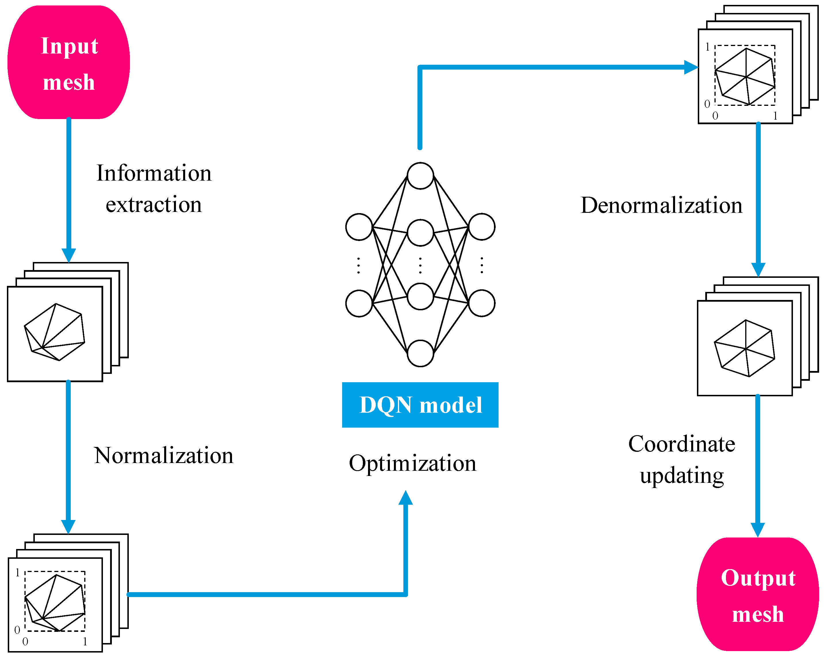
Figure 1.
Flow chart of the unconstrained DQN smoothing method.
Figure 1.
Flow chart of the unconstrained DQN smoothing method.
Figure 2.
Impact of the central node moving position on node quality. (a) Case 1, where the central node moves near the polygon boundary; (b) Case 1, where the central node moves near the polygon boundary; (c) Case 2, where the central node moves near the center of the polygon; (d) Case 2, where the central node moves near the center of the polygon.
Figure 3.
The construction process of the inner polygon. (a) The initial state of a polygon; (b) rotation angle and updated central node; (c) updated scatters; (d) convex hull processing for scattered points falling inside the polygon; and (e) the inner polygon constructed.
Figure 3.
The construction process of the inner polygon. (a) The initial state of a polygon; (b) rotation angle and updated central node; (c) updated scatters; (d) convex hull processing for scattered points falling inside the polygon; and (e) the inner polygon constructed.
Figure 4.
Workflow of the proposed angle and a deep Q-network-based mesh smoothing.
Figure 4.
Workflow of the proposed angle and a deep Q-network-based mesh smoothing.
Figure 5.
The data structure of mesh data information.
Figure 5.
The data structure of mesh data information.
Figure 6.
Changes in the size and position of the inner polygon. (a) The inner polygon when the center node is close to the polygon boundary; (b) The inner polygon when the central node moves towards the central region; (c) The inner polygon when the central node is close to the central region; (d) The inner polygon when the center node is located at the centroid of the polygon.
Figure 7.
Different types of polygons. (a) k = 3; (b) k = 4; (c) k = 5; (d) k = 6; (e) k = 7; (f) k = 8; (g) k = 9.
Figure 7.
Different types of polygons. (a) k = 3; (b) k = 4; (c) k = 5; (d) k = 6; (e) k = 7; (f) k = 8; (g) k = 9.
Figure 8.
Neural network performance analysis chart. (a) The growth curve of average Q-value with training epochs; (b) the growth curve of average reward with training epochs.
Figure 8.
Neural network performance analysis chart. (a) The growth curve of average Q-value with training epochs; (b) the growth curve of average reward with training epochs.
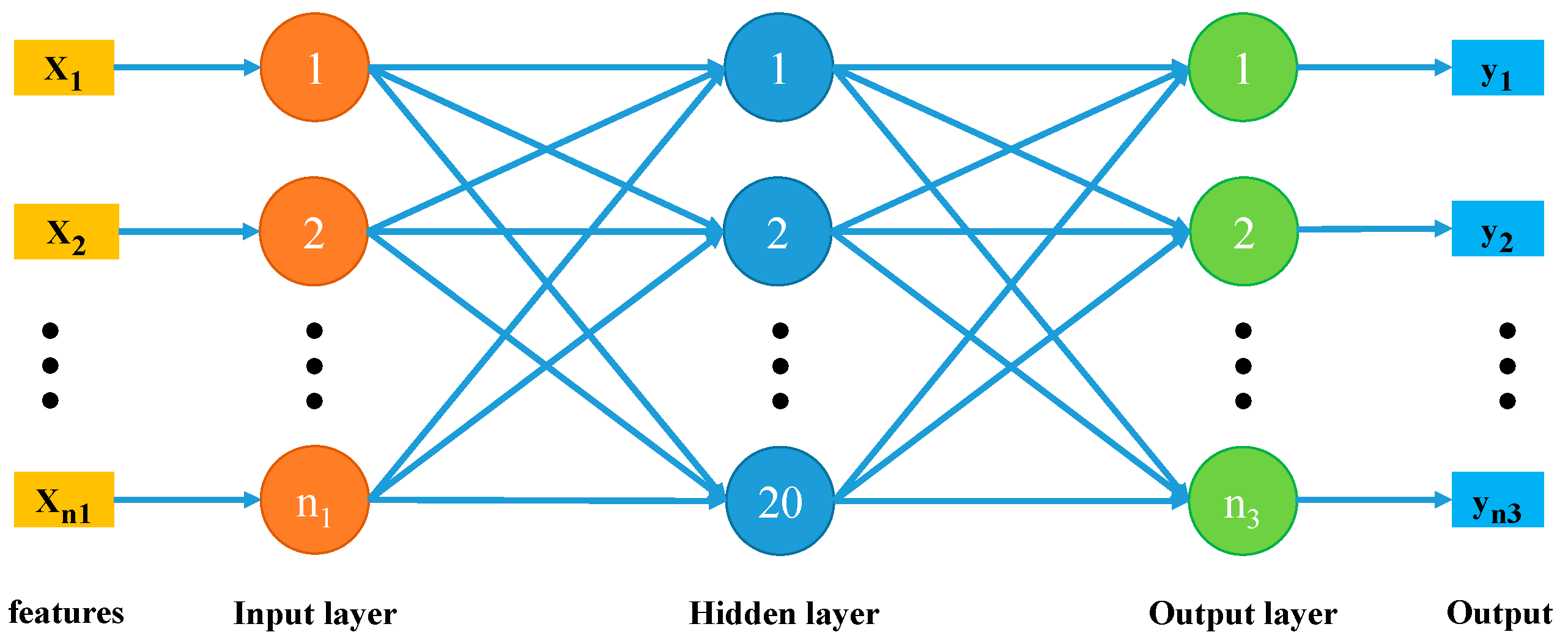
Figure 9.
Schematic diagram of neural network structure.
Figure 9.
Schematic diagram of neural network structure.
Figure 10.
Example 1 smoothing front-back diagram. (a) Before smoothing; (b) after smoothing.
Figure 10.
Example 1 smoothing front-back diagram. (a) Before smoothing; (b) after smoothing.
Figure 11.
Node quality convergence graph.
Figure 11.
Node quality convergence graph.
Figure 12.
Inner polygon convergence graph.
Figure 12.
Inner polygon convergence graph.
Figure 13.
Effectiveness of Example 2 comparison before and after smoothing. (a) Before smoothing; (b) after smoothing.
Figure 13.
Effectiveness of Example 2 comparison before and after smoothing. (a) Before smoothing; (b) after smoothing.
Figure 14.
Effectiveness of Example 3 comparison before and after smoothing. (a) Before smoothing; (b) after smoothing.
Figure 14.
Effectiveness of Example 3 comparison before and after smoothing. (a) Before smoothing; (b) after smoothing.
Figure 15.
Effectiveness of Example 4 comparison before and after smoothing. (a) Before smoothing; (b) after smoothing.
Figure 15.
Effectiveness of Example 4 comparison before and after smoothing. (a) Before smoothing; (b) after smoothing.
Figure 16.
Generalizability analysis of constrained DQN models. (a) Minimum angle contrast; (b) maximum angle contrast; (c) minimum quality contrast; (d) and average quality contrast.
Figure 16.
Generalizability analysis of constrained DQN models. (a) Minimum angle contrast; (b) maximum angle contrast; (c) minimum quality contrast; (d) and average quality contrast.
Figure 17.
Model generalization analysis chart.
Figure 17.
Model generalization analysis chart.
Figure 18.
Initial mesh. (a) Example 1; (b) Example 2; (c) Example 3; and (d) Example 4.
Figure 18.
Initial mesh. (a) Example 1; (b) Example 2; (c) Example 3; and (d) Example 4.
Figure 19.
The mesh after smoothing using the method in this paper. (a) Example 1; (b) Example 2; (c) Example 3; (d) and Example 4.
Figure 19.
The mesh after smoothing using the method in this paper. (a) Example 1; (b) Example 2; (c) Example 3; (d) and Example 4.
Figure 20.
Example 1—local comparison of each method after smoothing. (a) Laplacian; (b) angle-based; (c) ODT; (d) CVT; (e) unconstrained DQN; and (f) constrained DQN.
Figure 20.
Example 1—local comparison of each method after smoothing. (a) Laplacian; (b) angle-based; (c) ODT; (d) CVT; (e) unconstrained DQN; and (f) constrained DQN.
Figure 21.
Example 2—local comparison of each method after smoothing. (a) Laplacian; (b) angle-based; (c) ODT; (d) CVT; (e) unconstrained DQN; and (f) constrained DQN.
Figure 21.
Example 2—local comparison of each method after smoothing. (a) Laplacian; (b) angle-based; (c) ODT; (d) CVT; (e) unconstrained DQN; and (f) constrained DQN.
Figure 22.
Example 3—local comparison of each method after smoothing. (a) Laplacian; (b) angle-based; (c) ODT; (d) CVT; (e) unconstrained DQN; and (f) constrained DQN.
Figure 22.
Example 3—local comparison of each method after smoothing. (a) Laplacian; (b) angle-based; (c) ODT; (d) CVT; (e) unconstrained DQN; and (f) constrained DQN.
Figure 23.
Example 4—local comparison of each method after smoothing. (a) Laplacian; (b) angle-based; (c) ODT; (d) CVT; (e) unconstrained DQN; and (f) constrained DQN.
Figure 23.
Example 4—local comparison of each method after smoothing. (a) Laplacian; (b) angle-based; (c) ODT; (d) CVT; (e) unconstrained DQN; and (f) constrained DQN.
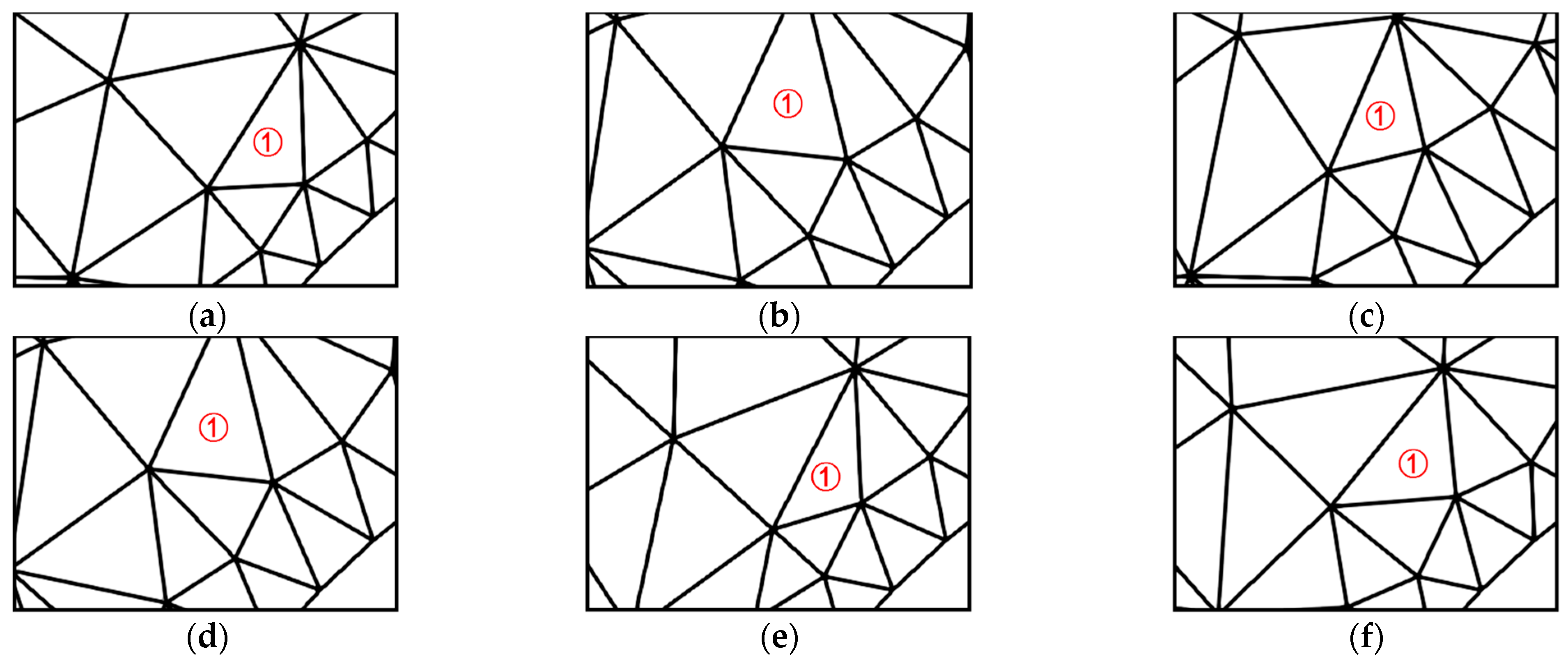
Figure 24.
Distribution of quality between 0.5 and 0.8.
Figure 24.
Distribution of quality between 0.5 and 0.8.
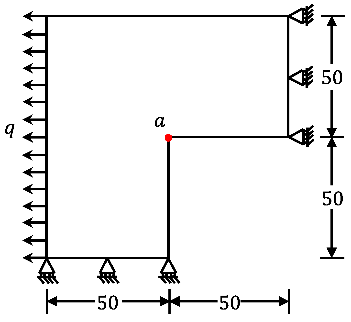
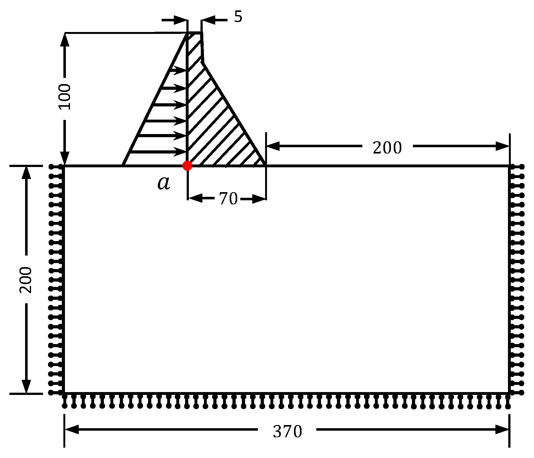
Figure 25.
L-shaped flat plate.
Figure 25.
L-shaped flat plate.
Figure 26.
Initial mesh, overall refined mesh, and optimized mesh. (a) Before smoothing; (b) refined mesh; and (c) after smoothing.
Figure 26.
Initial mesh, overall refined mesh, and optimized mesh. (a) Before smoothing; (b) refined mesh; and (c) after smoothing.
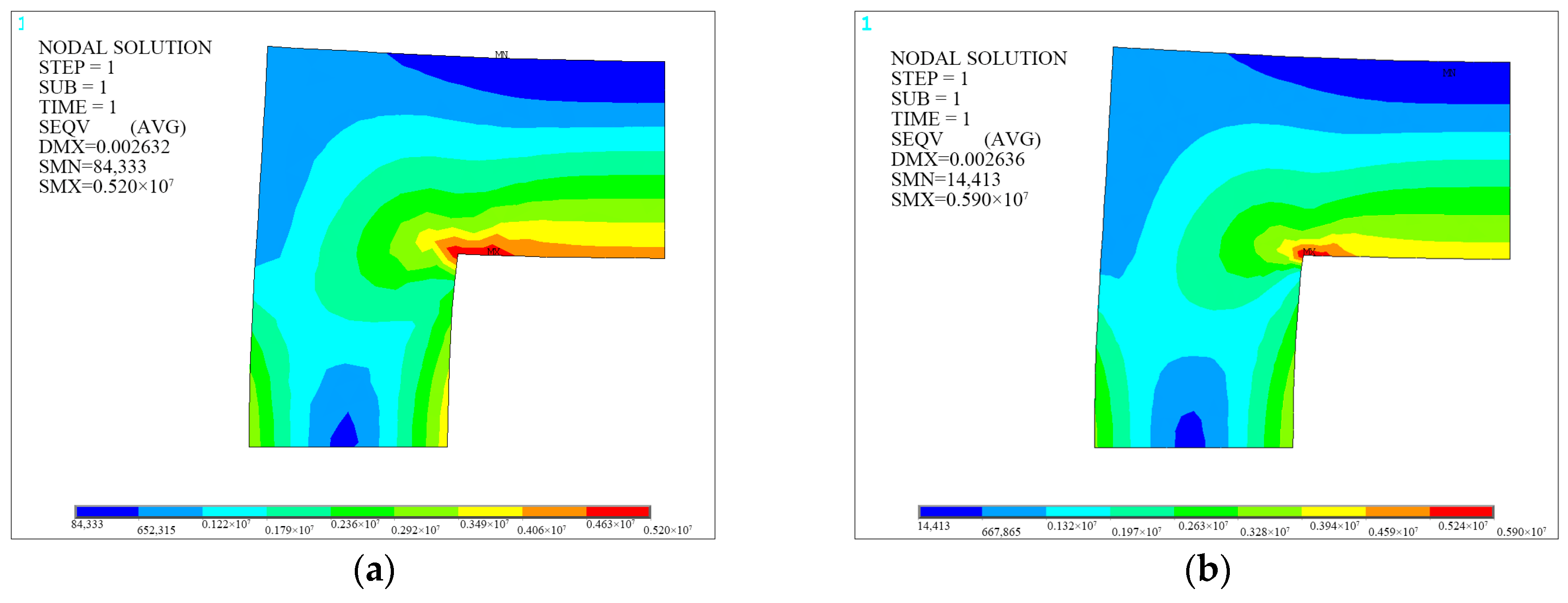
Figure 27.
Finite element calculation results of Example 1. (a) Initial mesh; (b) refined mesh.
Figure 27.
Finite element calculation results of Example 1. (a) Initial mesh; (b) refined mesh.
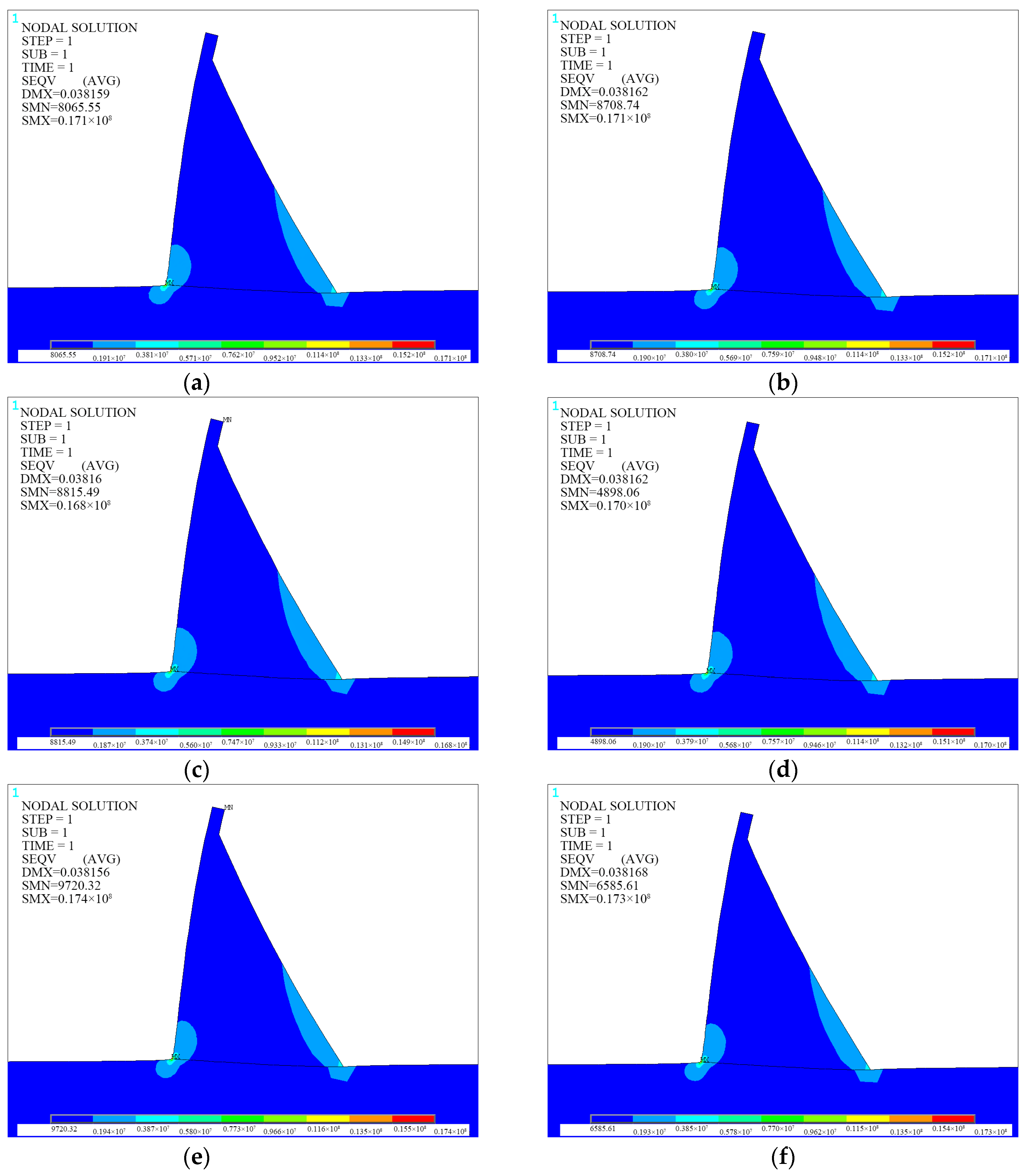
Figure 28.
Example 1: finite element calculation results after smoothing for each optimization method. (a) Laplacian; (b) angle-based; (c) ODT; (d) CVT; (e) unconstrained DQN; and (f) constrained DQN.
Figure 28.
Example 1: finite element calculation results after smoothing for each optimization method. (a) Laplacian; (b) angle-based; (c) ODT; (d) CVT; (e) unconstrained DQN; and (f) constrained DQN.
Figure 30.
Example 2—comparison before and after smoothing. (a) Before smoothing; (b) after smoothing.
Figure 30.
Example 2—comparison before and after smoothing. (a) Before smoothing; (b) after smoothing.
Figure 31.
Finite element calculation results of the initial mesh. (a) Global; (b) local.
Figure 31.
Finite element calculation results of the initial mesh. (a) Global; (b) local.
Figure 32.
Example 2: finite element calculation results after smoothing for each optimization method. (a) Laplacian; (b) angle-based; (c) ODT; (d) CVT; (e) unconstrained DQN; and (f) constrained DQN.
Figure 32.
Example 2: finite element calculation results after smoothing for each optimization method. (a) Laplacian; (b) angle-based; (c) ODT; (d) CVT; (e) unconstrained DQN; and (f) constrained DQN.
Table 1.
Reward function setting for DQN model.
Table 1.
Reward function setting for DQN model.
| State | Reward Function |
|---|
| Normal | |
| Node quality exceeds the threshold | 10 |
| The agent moves out of the inner polygon | −10 |
| The agent moves out of the polygon | −100 |
Table 2.
Table of parameter setting for neural networks.
Table 2.
Table of parameter setting for neural networks.
| Parameter | Symbol | Value |
|---|
| learning rate | | 0.01 |
| decay rate | | 0.9 |
| epsilon | | 0.9 |
| number of times experience pool D starts to replay | | 500 |
| batch size | | 32 |
| number of intervals for updating objective function | | 300 |
| maximum number of steps in a single round | | 200 |
| maximum number of rounds | | 1000 |
| optimizer | RMSProp |
| activation function | ReLU |
Table 3.
Table of comparison before and after mesh smoothing.
Table 3.
Table of comparison before and after mesh smoothing.
| Mesh | State | Nodes | Min. θ | Max. θ | Min. q | Avg. q |
|---|
| 2 | Before smoothing | 619 | 18.3706 | 129.4545 | 0.4802 | 0.8632 |
| After smoothing | 34.1760 | 99.4288 | 0.7810 | 0.9279 |
| 3 | Before smoothing | 426 | 17.8954 | 128.0146 | 0.5009 | 0.7906 |
| After smoothing | 34.9065 | 93.8188 | 0.8173 | 0.9361 |
| 4 | Before smoothing | 426 | 33.1073 | 98.6044 | 0.7962 | 0.9677 |
| After smoothing | 37.6581 | 91.6064 | 0.8517 | 0.9629 |
Table 4.
Comparison table of the experimental results.
Table 4.
Comparison table of the experimental results.
| Mesh | Method | Time/(s) | Nodes | Min. θ | Max. θ | (a) | (b) | Min. q | Avg. q |
|---|
| 1 | Initial | / | | 17.62 | 130.12 | 1434 | 1115 | 0.5001 | 0.7715 |
| Laplacian | 0.2886 | | 26.86 | 110.70 | 3 | 14 | 0.6495 | 0.9608 |
| Angle-based | 0.4520 | | 26.29 | 105.47 | 2 | 7 | 0.6840 | 0.9537 |
| ODT | 0.3890 | 2027 | 19.00 | 126.50 | 42 | 54 | 0.5125 | 0.9109 |
| CVT | 0.3390 | | 27.90 | 106.34 | 6 | 12 | 0.7249 | 0.9308 |
| Unconstrained DQN | 1.5944 | | 25.78 | 114.74 | 24 | 37 | 0.6479 | 0.9185 |
| Constrained DQN | 1.6218 | | 32.499 | 96.28 | 0 | 0 | 0.7944 | 0.9426 |
| 2 | Initial | / | | 10.49 | 146.45 | 158 | 117 | 0.2902 | 0.8481 |
| Laplacian | 0.1172 | | 28.05 | 110.21 | 6 | 7 | 0.6713 | 0.9239 |
| Angle-based | 0.1461 | | 21.67 | 106.68 | 28 | 11 | 0.5972 | 0.9096 |
| ODT | 0.1367 | 926 | 22.70 | 124.73 | 26 | 30 | 0.5517 | 0.9019 |
| CVT | 0.1211 | | 27.14805 | 114.34 | 4 | 12 | 0.6454 | 0.9154 |
| Unconstrained DQN | 0.3721 | | 26.05 | 104.54 | 2 | 6 | 0.6871 | 0.9179 |
| Constrained DQN | 0.3986 | | 29.25 | 100.25 | 1 | 1 | 0.7249 | 0.9208 |
| 3 | Initial | / | | 33.31 | 101.55 | 0 | 3 | 0.7713 | 0.9499 |
| Laplacian | 0.3666 | | 30.27 | 102.95 | 0 | 8 | 0.7166 | 0.9563 |
| Angle-based | 0.7174 | | 25.05 | 120.23 | 13 | 11 | 0.5888 | 0.9474 |
| ODT | 0.5078 | 2987 | 33.07 | 101.55 | 0 | 2 | 0.7713 | 0.9481 |
| CVT | 0.4544 | | 32.15 | 99.94 | 0 | 0 | 0.7850 | 0.9492 |
| Unconstrained DQN | 2.2742 | | 34.68 | 98.56 | 0 | 0 | 0.7978 | 0.9487 |
| Constrained DQN | 2.3175 | | 36.18 | 94.92 | 0 | 0 | 0.8229 | 0.9496 |
| 4 | Initial | / | | 17.67 | 130.17 | 3789 | 2908 | 0.5001 | 0.7686 |
| Laplacian | 1.1419 | | 26.00 | 109.88 | 3 | 14 | 0.6560 | 0.9630 |
| Angle-based | 1.6108 | | 23.23 | 103.44 | 16 | 17 | 0.6196 | 0.9560 |
| ODT | 1.5983 | 5115 | 19.56 | 128.79 | 64 | 69 | 0.5041 | 0.9367 |
| CVT | 1.4202 | | 24.03 | 105.90 | 11 | 24 | 0.6490 | 0.9486 |
| Unconstrained DQN | 3.6788 | | 23.97 | 117.88 | 29 | 41 | 0.6365 | 0.9127 |
| Constrained DQN | 3.7988 | | 32.31 | 100.77 | 0 | 2 | 0.7539 | 0.9465 |
Table 5.
Comparison table of the experimental results.
Table 5.
Comparison table of the experimental results.
| Mesh | Method | Time/(s) | Nodes | Min. θ | Max. θ | (a) | (b) | Min. q | Avg. q |
|---|
| 2 | Initial | / | | 26.93 | 108.78 | 45 | 86 | 0.7003 | 0.8635 |
| Laplacian | 0.1024 | | 28.62 | 102.80 | 3 | 2 | 0.7139 | 0.9417 |
| Angle-based | 0.2045 | | 28.82 | 100.26 | 2 | 1 | 0.7517 | 0.9475 |
| ODT | 0.1377 | 788 | 28.62 | 104.52 | 3 | 7 | 0.7139 | 0.9401 |
| CVT | 0.1249 | | 28.62 | 99.80 | 3 | 0 | 0.7139 | 0.9478 |
| Unconstrained DQN | 0.3175 | | 30.06 | 103.39 | 0 | 3 | 0.7403 | 0.9262 |
| Constrained DQN | 0.3261 | | 33.03 | 98.44 | 0 | 0 | 0.7954 | 0.9357 |
Table 6.
Errors in maximum stress of different optimized meshes.
Table 6.
Errors in maximum stress of different optimized meshes.
| Method | Nodes | Elements | Stress (Mpa) | Error (%) |
|---|
| Initial | | | 5.1531 | 12.5939 |
| Laplacian | | | 5.4915 | 6.8524 |
| Angle-based | | | 5.5006 | 6.6984 |
| ODT | 435 | 788 | 5.5068 | 6.5934 |
| CVT | | | 5.4987 | 6.7310 |
| Unconstrained DQN | | | 5.4453 | 7.6354 |
| Constrained DQN | | | 5.5564 | 5.7523 |
| Refinement | 804 | 1496 | 5.8955 | / |
Table 7.
Comparison table of the experimental results.
Table 7.
Comparison table of the experimental results.
| Mesh | Method | Time/(s) | Nodes | Min. θ | Max. θ | (a) | (b) | Min. q | Avg. q |
|---|
| 2 | Initial | / | | 8.32 | 153.96 | 1562 | 1095 | 0.2190 | 0.7312 |
| Laplacian | 0.6207 | | 26.52 | 111.37 | 12 | 24 | 0.6683 | 0.9507 |
| Angle-based | 0.6969 | | 26.52 | 111.32 | 11 | 21 | 0.6679 | 0.9411 |
| ODT | 0.7397 | 1665 | 14.30 | 148.60 | 27 | 40 | 0.3159 | 0.9336 |
| CVT | 0.8148 | | 16.93 | 135.92 | 25 | 32 | 0.6355 | 0.9437 |
| Unconstrained DQN | 1.2549 | | 27.09 | 127.17 | 33 | 30 | 0.5264 | 0.9188 |
| Constrained DQN | 1.3166 | | 31.01 | 108.64 | 0 | 2 | 0.6814 | 0.9372 |
Table 8.
Comparison table of finite element calculation results.
Table 8.
Comparison table of finite element calculation results.
| Method | Nodes | Element | Stress (x) | Error (x) | Stress (x) | Error (y) | Mean Error |
|---|
| Initial | 1665 | 3178 | 9.6259 | 30.25 | 10.2441 | 30.03 | 30.14 |
| Laplacian | 9.9706 | 27.75 | 10.9232 | 22.34 | 25.04 |
| Angle-based | 9.8940 | 28.30 | 10.9515 | 25.19 | 26.75 |
| ODT | 9.7165 | 29.59 | 10.6509 | 27.25 | 28.42 |
| CVT | 9.7404 | 29.42 | 10.8809 | 25.68 | 27.55 |
| Unconstrained DQN | 10.0845 | 26.92 | 11.2019 | 23.48 | 25.20 |
| Constrained DQN | 10.6940 | 22.51 | 11.8218 | 19.25 | 20.88 |
| Reference [30] | 8263 | 10,270 | 13.8000 | / | 14.6400 | / | / |


