1. Introduction
The COVID-19 pandemic has stimulated the growth of the e-commerce market, which is projected to exceed US
$6.388 trillion in 2024 with an annual growth rate of approximately 13.5% [
1]. In addition, the number of people who have used online shopping services has significantly increased, reaching 3 billion people in 2018, and this growth has further accelerated due to the challenges of pandemics [
2]. Last-mile logistics are a key point for addressing these bottlenecks. However, last-mile activities are costly and environmentally polluting, accounting for 13–75% of overall logistics costs [
3]. According to a report by Forum [
4], the number of delivery vehicles used is expected to increase by 36%, but effective solutions can lead to a 30% reduction in waste emissions and a nearly 25% decrease in total logistics costs. Logistics companies aim to offer diverse services along with faster deliveries to enhance customer satisfaction and reduce operating costs. Environmental concerns, such as noise and air pollution, prompt them to invest in and implement alternative systems [
5].
To effectively address environmental concerns, there is a growing trend to replace fuel-consuming vehicles with those powered by sustainable and renewable energy sources. Electric vehicles (EVs) are widely recognized as one of the cleanest transportation means for both private and commercial purposes that generate no local greenhouse gas (GHG) emissions and help reduce noise pollution. Therefore, logistics companies such as DHL, Amazon, and FedEx have already implemented fleets of EVs into their logistics networks. From the perspective of operation research, the use of EVs in last-mile delivery networks to serve customers is studied by ref. [
6], which establishes a more sustainable delivery network. Variants of the electric vehicle routing problem (EVRP) have been developed and extended over the past decade. Keskin and Çatay [
7] investigate recharge policies to tackle the limitations of battery capacities with shorter recharging durations, named the electric vehicle routing problem with time windows and partial recharges (EVRPTW-PR).
The conventional last-mile delivery method (i.e., home delivery method) faces various challenges in serving customers within the limitations of time windows and dealing with the possibility of customers being unavailable. Moreover, the problem of urban traffic congestion further causes delays in delivery. These factors contribute to a significant risk of delivery failures, resulting in increased air pollution and logistics costs and decreased customer satisfaction levels. Consequently, logistics companies investigate alternative delivery methods to overcome these challenges. One of the potential alternatives is the self-pickup method, wherein couriers drop customers’ parcels at assigned parcel lockers, allowing customers to conveniently retrieve their packages at any time. In practice, parcel locker systems used for delivery have been successfully installed and implemented in more than 20 countries, such as the U.S., UK, Germany, and Canada, which ensure reliable, responsive, and professional delivery experiences [
8]. In addition, this delivery method proves particularly suitable during a pandemic as it eliminates the need for direct customer interactions [
9].
From the perspective of operations research, we study the integration of parcel lockers into sustainable last-mile delivery networks so as to provide routing plans while minimizing logistics costs, called the electric vehicle routing problem with time windows, partial recharges, and parcel lockers (EVRPTW-PR-PL). While the concept of our study has also been explored by ref. [
10], our proposed network differs from them in two features: (1) the locations of parcel lockers and recharging stations (CSs) are distinguished, and (2) each customer is associated only with a designated parcel locker if the self-pickup method is offered. To sum up, our main contributions are highlighted as follows.
We study the implementation of parcel lockers based on the concepts of EVRPTW-PR, called the Electric Vehicle Routing Problem with Time Windows, Partial Recharges, and Parcel Lockers (EVRPTW-PR-PL).
We formulate a mixed-integer programming (MIP) model and design an adaptive large neighborhood search (ALNS) for solving both EVRPTW-PR and EVRPTW-PR-PL.
The performance of the proposed ALNS is shown by solving the EVRPTW-PR benchmark instances.
We provide some managerial insights from the implementation of parcel lockers.
The remaining parts of this study are structured as follows.
Section 2 reviews papers related to EVRPTW-PR and the implementation of parcel lockers.
Section 3 formulates MILP to solve EVRPTW-PR-PL along with a formal description.
Section 4 presents an ALNS algorithm that incorporates operators designed for addressing parcel lockers in the network.
Section 5 conducts numerical experiments related to ALNS performance and the implementation of parcel lockers.
Section 6 discusses the effects of parcel lockers on the problems. Finally, we give some conclusions and potential research in
Section 7.
3. Problem Description and Mathematical Model
With the presence of parcel lockers, there are two delivery methods offered, including (1) home delivery and (2) self-pickup at parcel lockers. With these delivery methods, we propose three types of customers for our problem. The first type is home delivery customers (H), who are required to directly receive parcels at their home locations. The second type is self-pickup customers (S), who come to the designated parcel lockers to pick up parcels. Each self-pickup customer is allowed to select a preferred parcel locker, which is convenient for collecting parcels. The last type is flexible customers (F), who are willing to be served by either home delivery or self-pickup methods. Note that the preferred delivery method for each customer is known in advance.
Let be a set of all customers (i.e., consisting of three subsets of home delivery, self-pickup, and flexible customers, respectively), P denotes a set of parcel lockers, F denotes the set of recharging stations (CSs), and is the origin and destination depots. We define EVRPTW-PR-PL as a directed graph , where the set of nodes N can be separated into subsets as . Note that set includes set F and its copies of each CS to allow multiple visits to CSs. For later formal expressions, we denote subsets , , , and . The set of arcs A is defined by . For each arc , travel cost and travel time are defined by and , respectively.
All customers are served by a homogeneous fleet of EVs (denoted by set K) with a load capacity of Q, battery capacity of B, and electric consumption rate of r. Each utilized EV starts at the depot with a fully charged battery and ends at the depot. During transportation, each EV is allowed to recharge its battery at CSs with a charging rate of g. Note that each CS may serve EVs multiple times. Furthermore, each parcel locker with a capacity limited by the number of customers (denoted by ) may serve several self-pickup and flexible customers and can be visited by one or more vehicles. Let denote the designated parcel locker of customer . Consequently, each parcel locker has a subset of associated customers , which represents the possible connection between the parcel locker and customers in the subset. Each customer has a predefined time window , a non-negative demand , and a service time . Demand and service time of the remaining vertices (i.e., parcel lockers and CSs) are set to 0, while their time windows are denoted by , with as the maximum duration of the routing plan.
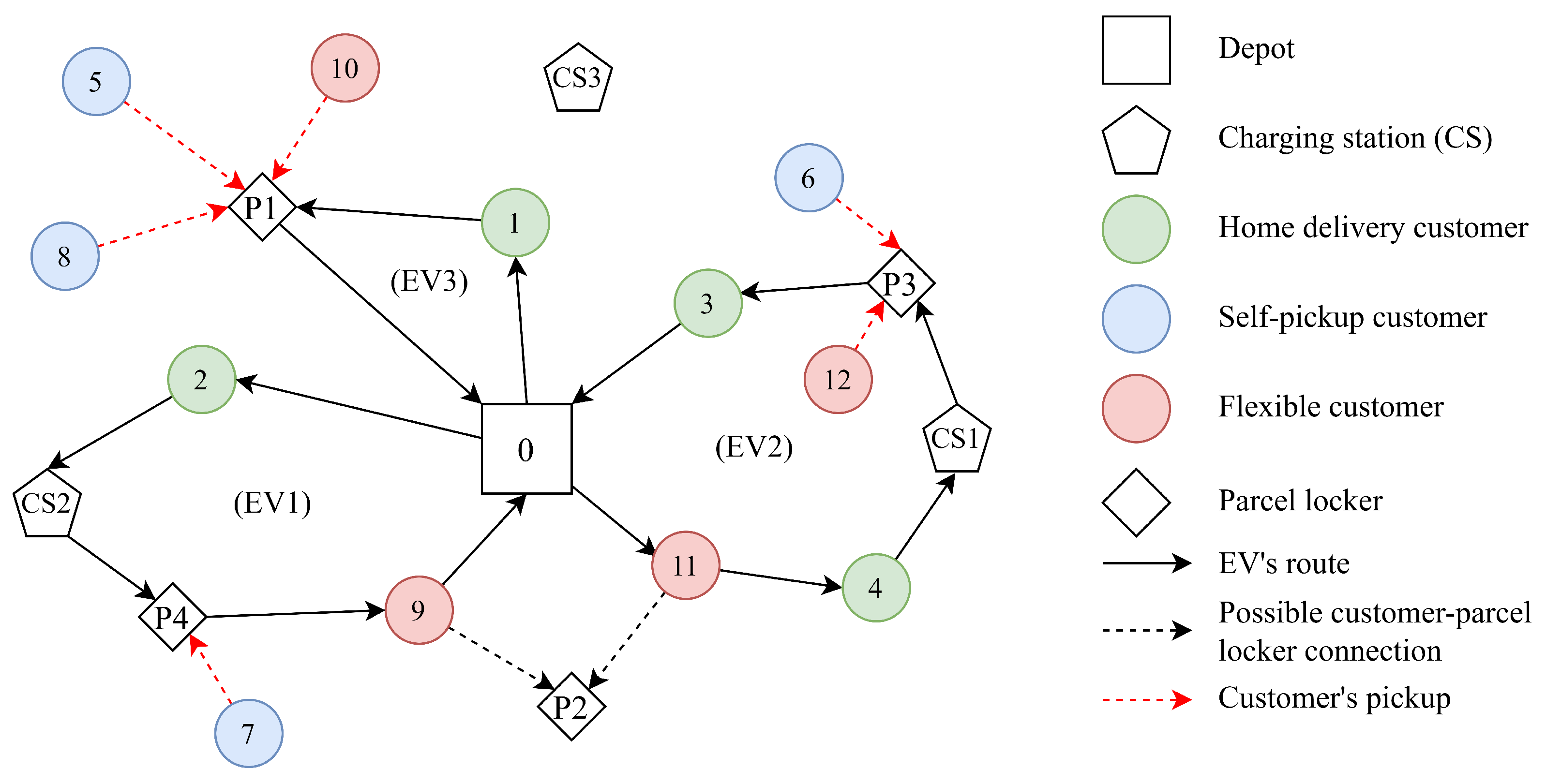
Figure 1 presents an illustrative network including 4 home delivery customers (1–4), 4 self-pickup customers (5–8), 4 flexible customers (9–12), 4 parcel lockers (P1–P4), 3 recharging stations (CS1–CS3), and depot 0. Regarding the self-pickup method, the sets of possible connections for parcel lockers are
,
,
, and
(see hash lines in
Figure 1). The figure depicts a routing plan for serving all customers along with their corresponding delivery methods by using three EVs. All home delivery customers have their parcels delivered to their homes, while self-pickup customers receive their parcels at parcel lockers (see red hashed lines in
Figure 1). Flexible customers 9 and 11 are not assigned to the self-pickup method (see black hashed lines in
Figure 1), while customers 10 and 12 take their orders from the parcel lockers. In particular, route 1 visits parcel locker P4 to drop off parcels for customer 7. Similarly, route 2 delivers parcels from customers 6 and 12 to parcel locker P3. Finally, route 3 involves a visit to parcel locker P1, where customers 5, 8, and 10 retrieve their parcels. Some CSs are also visited by EVs to recharge their batteries.
For seeking the routing plans on EVRPTW-PR-PL, the model uses the following decision variables: binary variable is equal to 1 if arc is traversed and 0 otherwise. Let for all be a binary variable equal to 1 if the self-pickup method is chosen for customer i and 0 otherwise (indicating the home delivery method). The non-negative variable for all then determines the total parcels delivered to the parcel locker i. Regarding the battery level, non-negative variables and present the battery state when coming to and departing from vertex , respectively. Finally, non-negative variables and track the service starting time and current load when the EV arrives at vertex .
The objective function (
1) minimizes the total travel distance of the EVs.
Constraints (
2) and (
3) enforce the associated delivery methods for all customers. Constraint (
4) addresses arc connectivity related to CSs. Constraint (
5) ensures that the parcel locker must be visited by vehicles if it keeps parcels for at least one customer. Constraint (
6) conserves EV’s flows at each node within routes. Constraint (
7) limits the number of used electric vehicles.
Constraints (
8) and (
9) track the starting time for serving at each node. Constraints (
10) and (
11) impose that vehicles can only visit nodes within their predefined time windows. The current loading of EVs at each node is recorded by constraints (
12) and (
13). Constraint (
14) guarantees that a vehicle’s total load does not exceed its capacity. Constraint (
15) states that the actual demand of each parcel locker equals the total demand from customers picking up their parcels at that specific parcel locker. Constraint (
16) limits that the number of customers assigned to each parcel locker does not exceed the parcel locker’s capacity. Constraint (
17) imposes that each self-pickup customer must be assigned to the self-pickup method.
Constraints (
18) and (
19) track the remaining battery capacity when the EVs visit CSs and the remaining nodes, respectively. Constraint (
20) ensures that the battery state of charge does not exceed its capacity at CSs.
4. Solution Method
To solve EVRPTW-PR-PL, we propose an ALNS algorithm that has successfully solved a broad range of routing problems, such as pickup and delivery problems [
48], the two-echelon vehicle routing problem (2E-VRP) [
49], VRP with handling uncertainty [
50], EVRP variants [
7,
51,
52], and VRP with delivery options (VRPDO) [
40]. Schiffer and Walther [
52] derive a set of functions to efficiently check the feasibility of EV routes in
time complexity. The efficient operators for handling delivery options described in one study [
40] are also utilized in our problem.
A solution of EVRPTW-PR-PL is represented by two arrays. Array 1 represents a set of sequences that include served customers who may visit some CSs in order. Array 2 is associated with array 1, which reports the delivery methods for customers. In particular, if a customer within array 1 is assigned to the self-pickup method, then the designated parcel locker is placed in the corresponding position of the customer in array 1; otherwise, the remaining positions are copied from array 1. Based on this representation, the preferred delivery methods are always ensured for all customers, and the total demand for parcel lockers is also guaranteed. However, it is possible for infeasible solutions to arise that can violate time window, battery, and load violations, resulting in penalties (see
Section 1). We note that total cost and penalties are determined based on the second array (see
Section 4.4).
Figure 2 presents the solution of the illustrative example (as shown in
Figure 1). With array 1, white cells represent home delivery customers and CSs, while blue and red cells represent self-pickup and flexible customers, respectively. Array 2 is then associated with array 1, where all blue cells must be replaced by the designated parcel lockers of self-pickup customers, and red cells can represent either the customers themselves or the designated parcel lockers. For example, route 2 is represented as
, where the flexible customer 11 is assigned to the home delivery method, while another flexible customer 12 is assigned to the self-pickup method at parcel locker 3 (as indicated in array 2). In addition, when two consecutive parcel lockers are the same on a route, we can combine them when updating the routes.
4.1. Construction Algorithm
Based on the structure of a solution representation, an initial solution for ALNS is generated by using a modified nearest neighborhood algorithm that includes two stages. In the first stage, we iteratively select the customer in the set of unassigned customers with the lowest cost increment (i.e.,
) and then insert it into the solution. The first stage terminates when all customers are served. In the second stage, an attempt is then made to reduce the battery violation by implementing the station insertion operator (see
Section 4.4.3).
To find the best insertion, all customers are tested to be inserted into all positions in the incomplete solution. The customer who results in the lowest cost increment is selected. It is important to note that the three types of customers are considered in different ways: (1) For home delivery customers: the customer locations are taken into account when evaluating cost increments; (2) For self-pickup customers: the designated parcel lockers are considered when evaluating cost increments; and (3) For flexible customers: both the aforementioned cases (i.e., home delivery and self-pickup) are considered when evaluating cost increments, resulting in a lower cost increment.
4.2. Evaluation of Penalties
To extend the search space, we accept infeasible solutions in terms of time windows, battery consumption, and vehicle loading, along with adding penalty costs [
53]. Let
denote a solution consisting of a set of
n routes. The generalized cost function of a solution
is denoted by
as follows. Next, the total cost function (
1) is generalized by taking into account three penalty terms related to time windows, battery, and vehicle load, as shown in the following expression.
Here,
is equivalent to the total cost (
1). Values
,
, and
denote the time window, battery, and load penalties, respectively. These penalties are included in the generalized total cost with associated weights
and
, which are initialized with
,
, and
. These weights are adjusted during the ALNS procedure with the ranges
, and
. Based on [
53], lower bounds are set as 0.5, and upper bounds are set as the objective value of the initial solution.
It is worth noting that dynamic penalty weights are used to reduce the occurrence of infeasible solutions during the execution of our ALNS procedure. More specifically, the penalty weights are increased to prevent infeasible solutions when the algorithm keeps failing to explore feasible solutions. This concept has been successfully implemented to solve EVRP variants such as [
52,
53,
54].
Load penalty
is easily determined in
time complexity [
55]. Battery and time window penalties are more challenging, but Schiffer and Walther [
52] propose an efficient approach by introducing a set of forward and backward variables. For the sake of calculations, all variables mentioned in this section are used in the same unit as travel time. We also introduce some supported parameters; i.e.,
denotes the recharge time with enough energy to traverse an arc
, and
denotes the time for recharging a full battery capacity. All variables are applied to concatenation operators for evaluating these penalties in
time complexity. In more detail, forward and backward functions are explained as follows.
4.2.1. Forward Functions
We introduce a set of variables for propagating from node
i to node
j. In particular, variable
(resp.
) denotes the earliest allowed arrival time adding the minimum required (resp. the maximum possible) charging time at previous CSs. Variables
and
replace
and
, respectively, when penalties occur in order to avoid over-penalization. In addition, slack time due to the waiting time before node
j is served results in the available time for charging, denoted by
. Variable
tracks the inverse residual battery capacity at node
j. Finally, variable
determines the minimum charging time in order to reach from node
i to node
j. Forward equations derived from [
52] are shown as follows. To shorten forward and backward functions, values
also involve service time at node
i.
At the starting depot 0, all values (i.e.,
,
,
,
, and
) are initialized as 0. Based on the above-mentioned variables, forward battery
and time window
penalties for each route
r are computed as follows.
4.2.2. Backward Functions
The backward variables consisting of
,
,
, as well as
and
are similarly used with the same terminology to update backward penalties. By considering an arc
, the backward variables are updated backwardly from node
j to node
i as the following equations.
4.2.3. Concatenation Operators
By utilizing forward and backward variables, concatenation operators allow us to obtain the penalties in
time complexity for two cases: (1) when inserting a node into a route, and (2) when removing a node from a route. However, when route segments (i.e., at least two vertices) are inserted, either forward or backward penalties have to be updated for the route segment first before implementing the two above-mentioned cases. (1) Insert a node
v into a route
V, expressed as
. There are two partial routes partitioned by node
v; i.e.,
and
. Forward and backward variables at node
v are calculated by Equations (
22)–(
28) and Equations (
31)–(
37), respectively. Time window violation (
) and battery violation (
) are then obtained as follows.
(2) Removing a node
v from a route
V, we obtain two partial routes
and
. First, forward variables at node
y are extended by Equations (
22)–(
28). Second, Equations (
42) and (
43) are derived to calculate the time windows and battery violations, respectively.
These operators never underestimate the total time window and battery violations, although the equations do not provide exact penalty values for each component.
4.3. Adaptive Large Neighborhood Search
Algorithm 1 presents our proposed ALNS, adopted by ref. [
52]. ALNS is an individual-based algorithm, which works on a current solution
initialized by the construction algorithm (see
Section 4.1). We set the current best solution
as
. While
accepts an infeasible solution,
records the current best feasible solutions. During the ALNS procedure, we utilize a temporary solution
to execute removal and insertion operators. The algorithm terminates when either of the two following conditions is met: (1) the algorithm reaches
iterations or (2) no improved solution is found after
iterations.
| Algorithm 1 ALNS pseudocode |
- 1:
- 2:
- 3:
if isFeasible then - 4:
- 5:
while do - 6:
- 7:
if random(0,1) < then - 8:
- 9:
- 10:
if then - 11:
- 12:
if then - 13:
- 14:
if isFeasible() then - 15:
- 16:
- 17:
else - 18:
- 19:
acceptanceWorse ▹ mentioned in Section 4.5 - 20:
if then - 21:
updatePenaltyWeights() - 22:
if then - 23:
updateSelectionProb() - 24:
- 25:
return
|
Each iteration starts by implementing
customerRemovalInsertion() into the temporary solution and then applying
lockerRemovalInsertion() with a probability of
. After that,
stationremovalinsertion() is executed to complete the removal and insertion phases. The obtained temporary solution
is then compared with the updated solutions in ALNS: (1)
replaces
if
is better than
, (2)
also replaces
if
is better than
, and (3) if a better feasible solution is obtained, then
is updated with
. These conditions govern the updating process at each iteration. However, we still accept a worse solution
to be
with a probability based on the temperature
T, denoted by
acceptanceWorse (see
Section 4.5).
Dynamic parameters are then updated based on the performance of operators. The penalty weights are updated (
updatePenaltyWeights()) based on the following. If no violation occurs within
iterations, then the associated penalty weight is divided by a constant
; otherwise, the penalty weight is multiplied by
. Similarly, the probability of removal and insertion operators is updated (
updateSelectionProb()) after
consecutive iterations (see
Section 4.4). Before proceeding to the next iteration, the temperature of the acceptance criteria is updated with a cooling rate of
. We note that the cooling rate
and the initial SA temperature
are from [
53].
4.4. Removal and Insertion Algorithms
This section introduces three classes of removal and insertion algorithms to address the features of our problem, i.e., the solution representation takes into account not only customer nodes, but also parcel lockers and recharging stations (CSs). Removal and insertion algorithms associated with customers are first presented in
Section 4.4.1.
Section 4.4.2 then introduces removal and insertion mechanisms designed for parcel lockers. Finally,
Section 4.4.3 proposes station removal and insertion algorithms, which exclusively consider recharging stations.
4.4.1. Customer Removal and Insertion
Customers are removed from the solution by three removal operators, while they are re-inserted into the solution by three insertion operators based on array 1 of the solution representation (denoted by
customerRemovalInsertion()). The customer removal and insertion algorithms are selected in an adaptive manner [
53]. The probabilities of selections are re-computed by a smoothing rate
after a learning period (i.e.,
iterations). During a learning period, when a new solution is generated, the associated removal and insertion algorithms are rewarded based on their performance. The rewards, denoted as
and
, correspond to different scenarios, which are gained when a new best feasible solution, a new best solution (which may be infeasible), a solution improving the current solution, and a worse solution, respectively, are found.
For each customer removal operator, customers are removed. The number of removed customers is randomly selected within a range . The following removal operators are implemented in our ALNS:
Random removal randomly removes customers from a given solution.
Worst removal is adopted by ref. [
53], which iteratively removes the customer that increases the generalized total cost the most, defined by
, where
and
represent the generalized costs before and after removing the customer, respectively. Moreover, to avoid being trapped at local optimum points, we consider randomness by controlling a randomness level
. Instead of choosing the highest cost reduction, the
-th highest cost reduction is then selected for removal from the solution, where
r is a random variable drawn from a uniform distribution
, and
is a list of customers sorted in descending order by the cost reduction.
Shaw removal was first introduced in [
56] and aims to remove customers that are similar to each other with respect to four criteria (i.e., travel distance, time window, demand, and delivery method). The procedure begins by randomly removing a customer and storing it in a list (denoted by
). The removal process is then repeated until
customers are removed. At every iteration, a customer
j in the route is selected for removal based on its relatedness to a randomly chosen customer
i from the list
. The relatedness between customers
i and
j is evaluated using the following equation:
Here, the four terms correspond to the relatedness of travel distance, the earliest time, demand, and delivery method, respectively. For the first three terms, each criterion is weighted by and , respectively. In addition, equals 0 if both customers are assigned the same delivery method (either home delivery or self-pickup method) and 1 otherwise. We note that a lower represents more relatedness between customers i and j.
For each insertion operator, the set of absent customers due to the removals is re-inserted into the solution. Infeasible solutions in terms of time windows, load, and battery are taken into account by the generalized objective function (see
Section 4.2). The insertion operators are briefly described as follows.
Greedy insertion is adopted by ref. [
48] and iteratively selects a customer from the list of absent customers with the best insertion for inserting into the solution until all customers are re-inserted. In each iteration, the customer with the best insertion is determined based on the increase in the generalized objective value. Note that for the home delivery method, customer locations are considered for insertion, while for the self-pickup method, parcel locker locations are taken into account.
k-regret insertion was first described by ref. [
48] and aims to anticipate the future impact of insertion operations. The process involves iteratively inserting the set of absent customers based on their regret-
k cost value. The regret-
k value of a customer is determined by calculating the difference between the sum of costs for inserting the customer in the
n-th lowest-cost position (denoted by
, given
) and the cost of inserting the customer in the lowest-cost position (denoted by
). Our paper implements this operator with
and
.
4.4.2. Locker Removal and Insertion
We adopt a procedure developed in the literature [
40] for handling the self-pickup method. This procedure involves locker removal and re-insertion into the solution based on array 2 of the solution representation, denoted by
lockerRemovalInsertion(). Note that the locker removal and insertion heuristics must be implemented together to effectively handle the self-pickup method. In particular, a parcel locker is first removed from the solution, which consists of one or more associated customers. We then obtain a list of removed customers. Subsequently, all customers with the designated parcel locker are re-inserted by using a locker insertion procedure. Locker removal and insertion mechanisms are presented as follows:
Locker removal as adopted by ref. [
40] is employed to prevent unnecessary repetition of customer removal and insertion operators without yielding any improvement. The procedure begins by recording all utilized parcel lockers in the considered solution that can potentially be removed. Next, a parcel locker is selected based on the highest reduction in distance cost when it is removed from the solution. Note that the parcel locker is removed, resulting in the removal of one or more associated customers.
Figure 3 provides an example illustrating the implementation of locker removal, as described in
Figure 2. In particular, there are three parcel locker positions (i.e., P4 in route 1, P3 in route 2, and P1 in route 3), as indicated by the red boxes in
Figure 3a.
Figure 3b shows the incomplete solution after removing parcel locker 3 in route 2.
Locker insertion is similar to customer greedy insertion, but with the key distinction that it exclusively considers the self-pickup method for inserting customers into the solution. Notably, the set of absent customers is designated to a single parcel locker.
4.4.3. Station Removal and Insertion
The recharging stations (CSs) are an important component of the problem. Thus, station removal and insertion heuristics are proposed to improve the solution in terms of battery violations, which are discussed as follows.
Station removal is similar to the worst customer removal. In this case, CSs are targeted for removal instead of customer nodes. This heuristic removes a specified number of stations, denoted as , which is determined by , where represents the total number of CSs existing in the solution.
Station insertion is similar to the greedy customer insertion for inserting CSs into the solution until no further improvement is found.
4.5. Acceptance Criteria
In our ALNS, we employ the simulated annealing (SA) acceptance criteria to escape local optima [
53]. In particular, not only are improved solutions accepted, but worse solutions are also accepted with a probability depending on the relative difference between
, and
, as well as the SA temperature.
Since infeasible solutions are allowed with dynamic penalty weights
, the generalized cost strongly depends on the values of penalty weights. Let
represent the penalty weights used for evaluating
and
represent the penalty weights used for evaluating
. To compare the generalized cost between
and
, we normalize the penalty weights as follows.
The probability of accepting a worse solution
is finally determined as follows.
Here, denotes the relative difference between the cost values of and .
The initial SA temperature and cooling rate are determined by following [
53]. Specifically, the initial SA temperature is configured so that a solution worse than the initial solution by 30% is accepted with a probability of 50%. In addition, the cooling rate is defined to limit the decrease in the temperature to below 0.0001 in the final 20% of iterations.
6. Discussion
We further conduct an evaluation to compare the results obtained from EVRPTW-PR and EVRPTW-PR-PL (with
) in terms of the cost ratio “CR” and the difference in the number of used vehicles
. The cost ratio “CR” is computed as the ratio between the best cost value
of EVRPTW-PR and the best cost value
of EVRPTW-PR-PL. The difference in used vehicles
is calculated as the number of used vehicles
in EVRPTW-PR minus the number of used vehicles
in EVRPTW-PR-PL. Therefore, in
Table A8,
Table A9,
Table A10,
Table A11,
Table A12,
Table A13,
Table A14,
Table A15 and
Table A16, we recall the results of EVRPTW-PR instances in
Section 5.3 and report terms “CR” and
in the right-most columns.
A summary of the results of the average cost ratio “CR” and the average difference in the number of used vehicles for each subset is provided in
Table 5. For the results from the large-sized instances, the patterns of “CR” and
are illustrated in
Figure 7 by sorting the subsets in ascending order of “CR” values. The figure helps highlight some features, as follows.
The implementation of parcel lockers in delivery networks significantly reduces travel costs for routing plans; i.e., the overall cost ratio is 1.72.
Figure 8 provides routing plans obtained from instance c101 for EVRPTW-PR and EVRPTW-PR-PL, which illustrates the differences between the two routing plans.
Considering customer locations, subsets with randomly distributed locations (i.e., subsets (R) and (RC)) show higher “CR” values. For example, the “CR” value for subset C-1 is only 1.08, while those for subsets R-1 and RC-1 are 1.38 and 1.66, respectively. This implies that utilizing parcel lockers becomes more effective when the locations are randomly scattered.
Considering time windows, subsets with wider customer time windows (i.e., C-1, R-1, and RC-1 subsets) provide higher “CR” values than those with stricter time windows (i.e., C-2, R-2, and RC-2 subsets). This means that instances with wider customer time windows have more potential to find cost-effective solutions when implementing parcel lockers.
Values of are not significant for all subsets; i.e., 0.07 vehicles on average. However, for subset R-1, the number of used vehicles is significantly reduced by 2.25 vehicles. This occurs when the customer locations are randomly distributed and the time windows are wider.
The insights noted above can be valuable in reality for delivery companies when making decisions regarding the deployment of parcel lockers in their last-mile delivery networks, aiming to leverage the cost-saving benefits. Specifically, companies can prioritize implementing parcel lockers in areas that reflect customer location patterns of “R” and “RC” subsets, as doing so provides great potential for cutting travel costs.
7. Conclusions
This paper addresses an extension of EVRPTW-PR by adding the self-pickup method for serving customers. As a result, there are three types of customers considered: (1) home delivery customers, (2) self-pickup customers, and (3) flexible customers. We formulate a mixed-integer programming (MIP) model and develop an ALNS algorithm adopted by ref. [
52] for efficiently solving both EVRPTW-PR and EVRPTW-PR-PL instances. Numerical experiments are conducted to test the performance of our proposed ALNS.
To provide comprehensive managerial insights regarding the implementation of parcel lockers in delivery networks, we have conducted sensitivity analyses based on the results obtained from EVRPTW-PR and EVRPTW-PR-PL. From our observations, the utilization of parcel lockers can lead to additional cost reductions in serving customers. The extent of cost reduction is influenced by various factors, such as the time windows and locations of customers in each instance. Furthermore, in subset R-1, where customer locations are randomly distributed and wider time windows are provided, we observe a decrease in the number of used vehicles for routing plans.
The generality of our algorithm could help tackle other similar problems. For instance, customers’ compensation schemes can be investigated by modifying the objective function, which would support policymakers to incentivize customers and enhance delivery network sustainability. Moreover, the cost of allocating parcel locker facilities can be included in the objective function. This provides a more comprehensive model that would help delivery companies make decisions for designing last-mile delivery networks with the use of parcel lockers. However, our research still has some limitations: (1) the scope of the study is limited to analyzing benchmark instances, and no real-world instances have been studied; and (2) the evaluation of the algorithm’s performance is challenging due to a lack of results from the existing algorithms or benchmarks for EVRPTW-PR-PL instances.
Some potential future research directions are as follows. First, alternative delivery locations and customers’ compensation schemes can be investigated to address a more comprehensive delivery network. More specifically, we could add additional costs (i.e., fixed costs for lockers and compensation costs) to the objective function to align with practical businesses. This model would help policymakers decide compensation strategies for more efficient routing plans and enhance customer satisfaction. Second, in realistic scenarios, the impacts of uncertain factors (e.g., travel time and charging/discharging consumption rates) are also worth studying to capture hidden costs within overall delivery costs. This also poses an interesting challenge through the implementation of stochastic programming or robust optimization. Finally, the applicability of our proposed problem can be enhanced by addressing practical delivery networks and offering more managerial insights.


