

A Novel Remaining Useful Life Probability Prediction Approach for Aero-Engine with Improved Bayesian Uncertainty Estimation Based on Degradation Data
Abstract
:1. Introduction
- An RUL probability prediction neural network based on degradation data is proposed for an aero-engine based on a BiGRU network and an IVBI technology, which can give not only the RUL prediction but also an accurate estimate of prediction uncertainties.
- A new IVBI method is proposed by replacing the traditional single Gaussian distribution in the variational Bayesian inference with a Gaussian mixture distribution to improve the generalization capability and prediction ability of the proposed method.
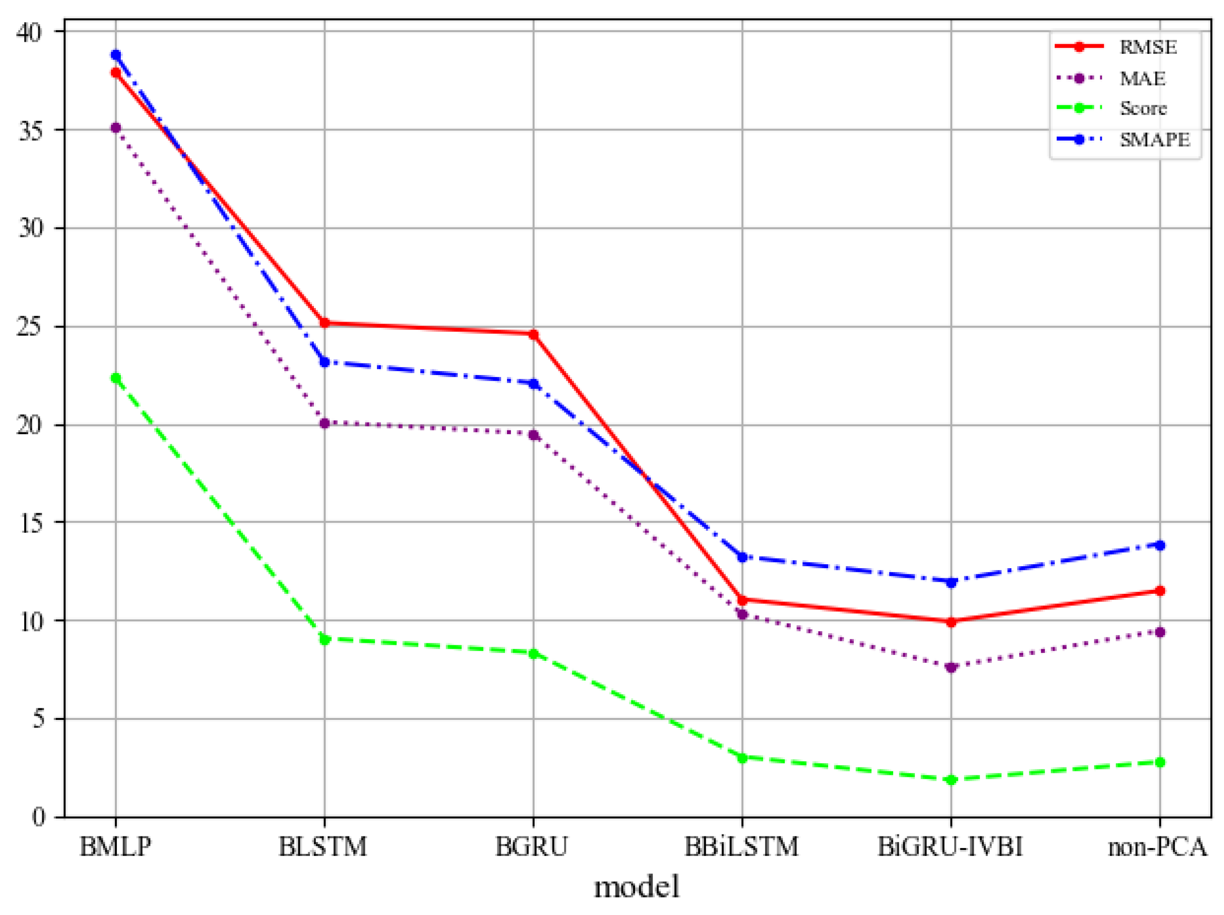
- The performance of the proposed model is validated on the CMAPSS data set. Comparisons with five other advanced deep learning methods show that our method is the most effective one under all of the considered evaluation indices.
2. The Proposed Method
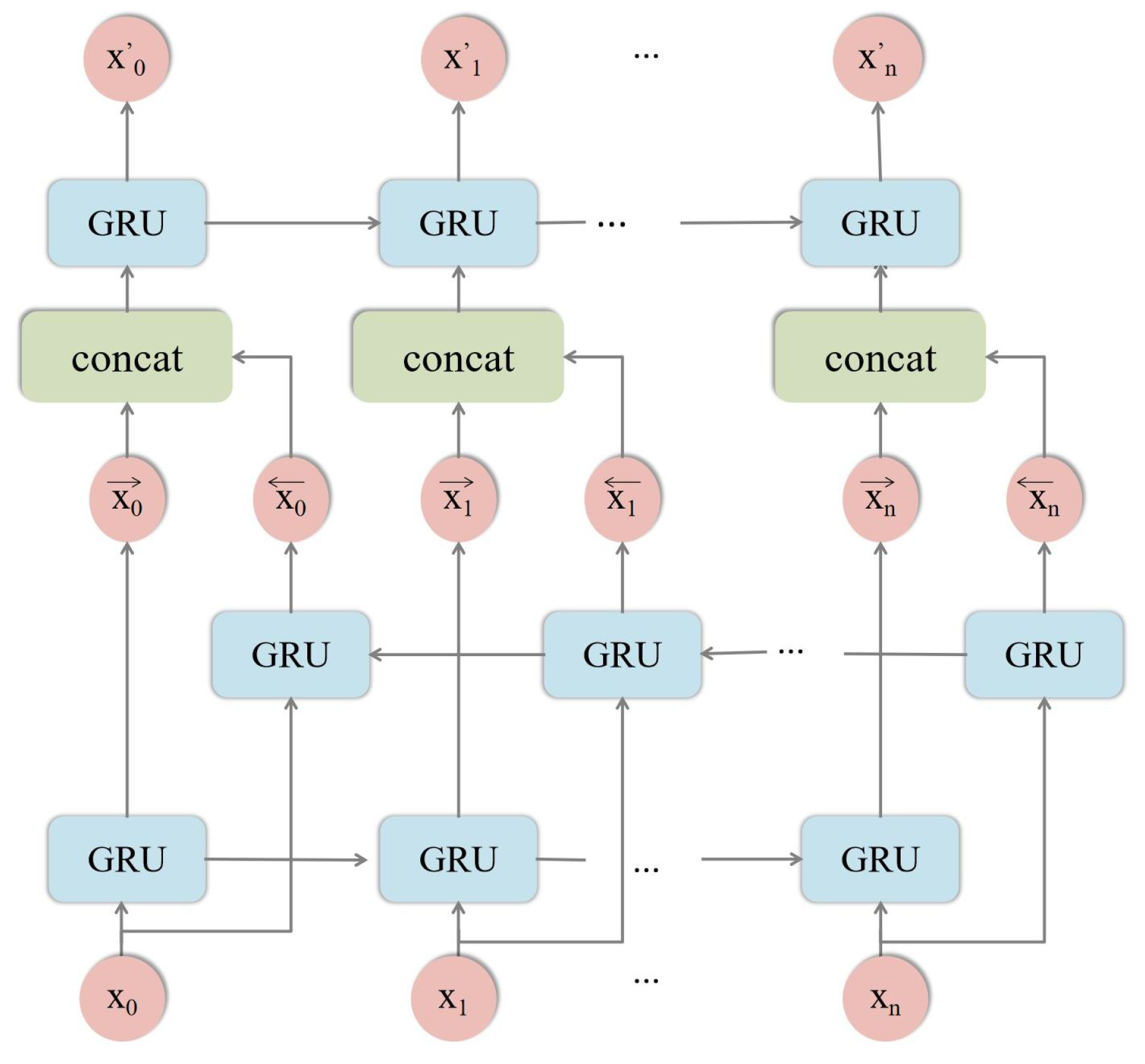
2.1. Bidirectional Gate Recurrent Unit
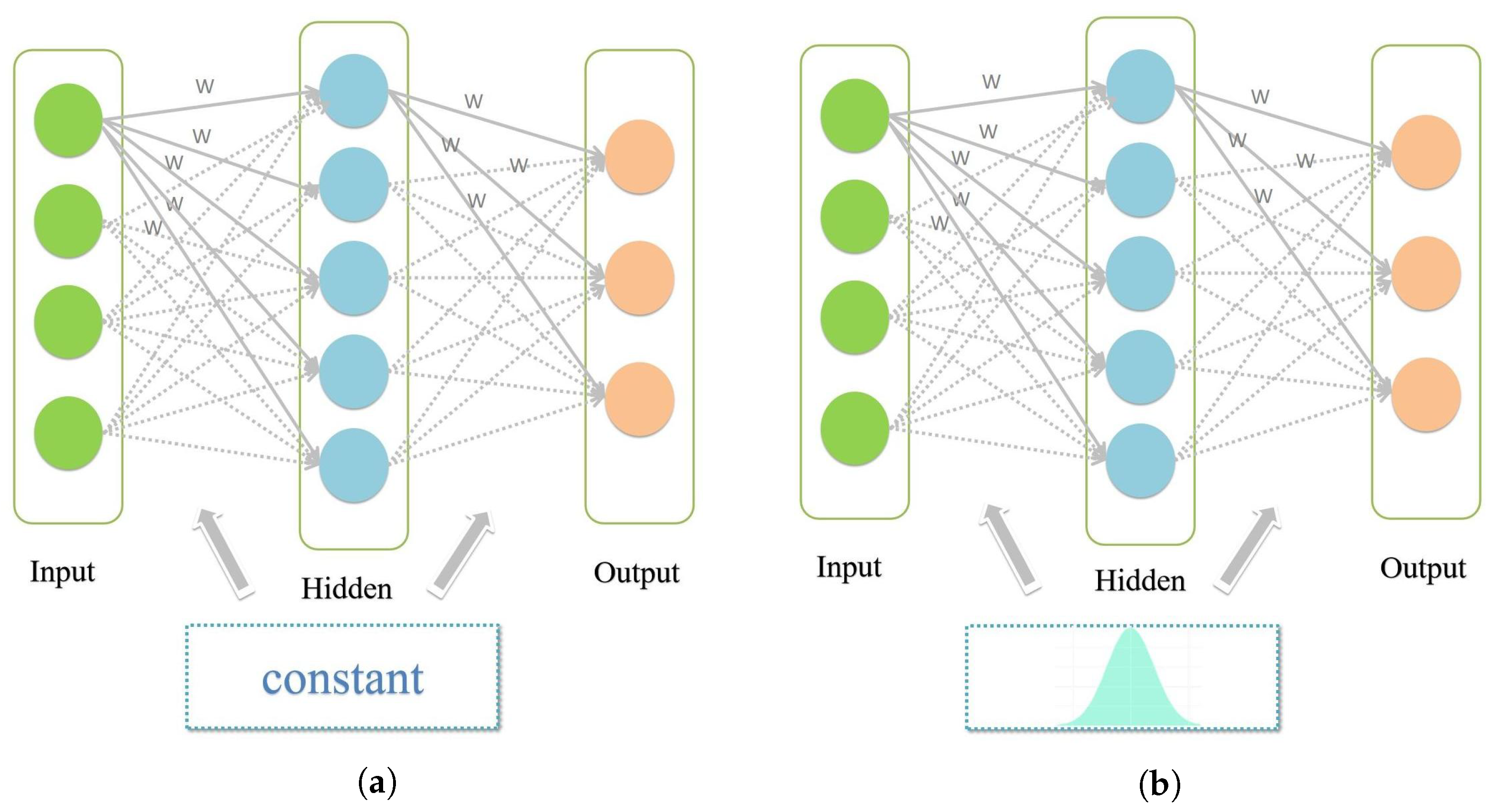
2.2. Bayesian Neural Network and Improved Variational Inference
- Improved hypothetical prior distribution
- Distribution difference measurement
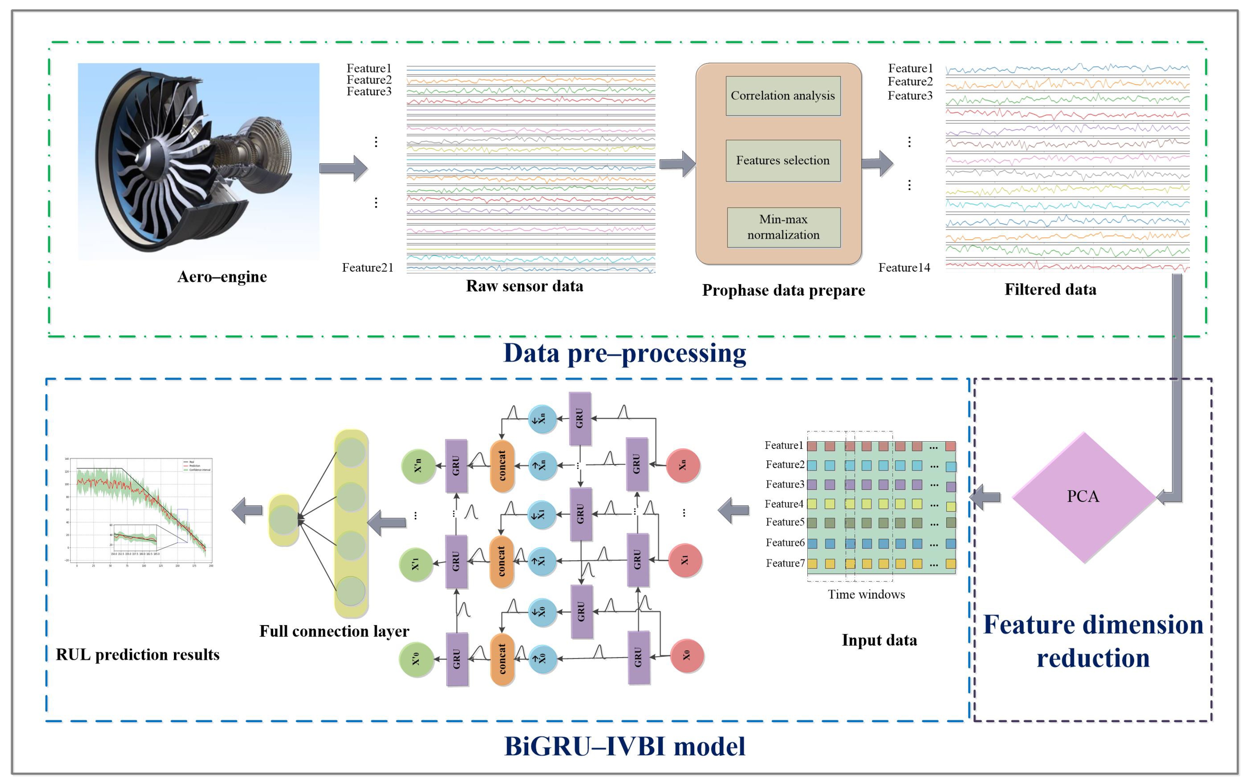
2.3. The RUL Probability Prediction Framework
3. Experimental Study
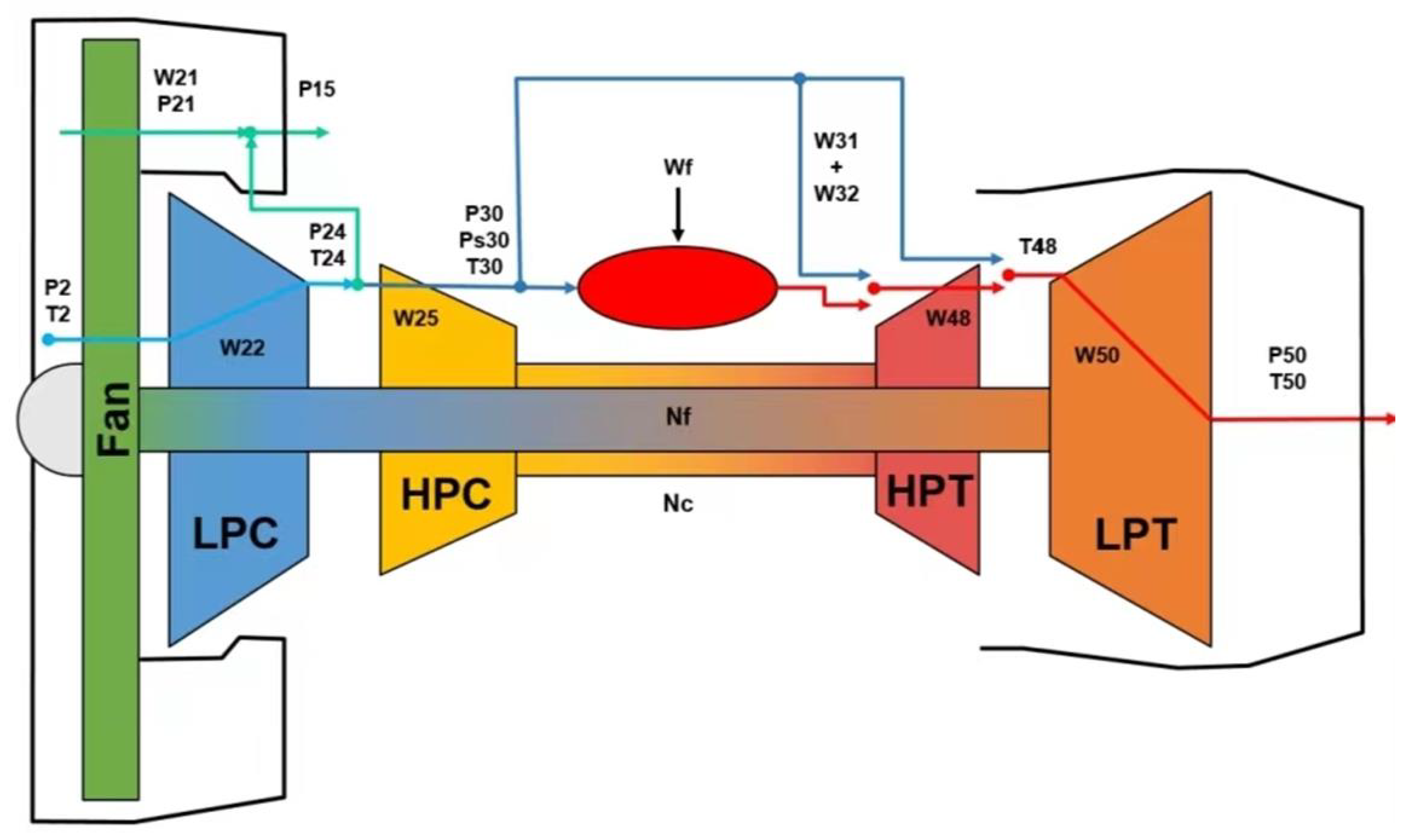
3.1. Data Description
3.2. Data Pre-Processing
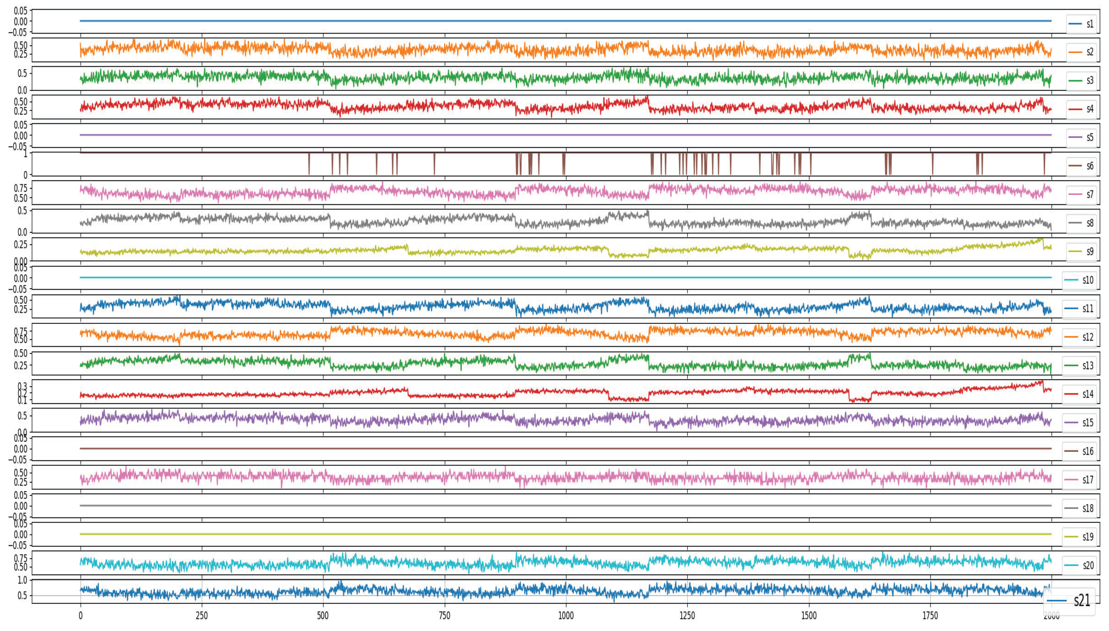
- Data visualization and analysis
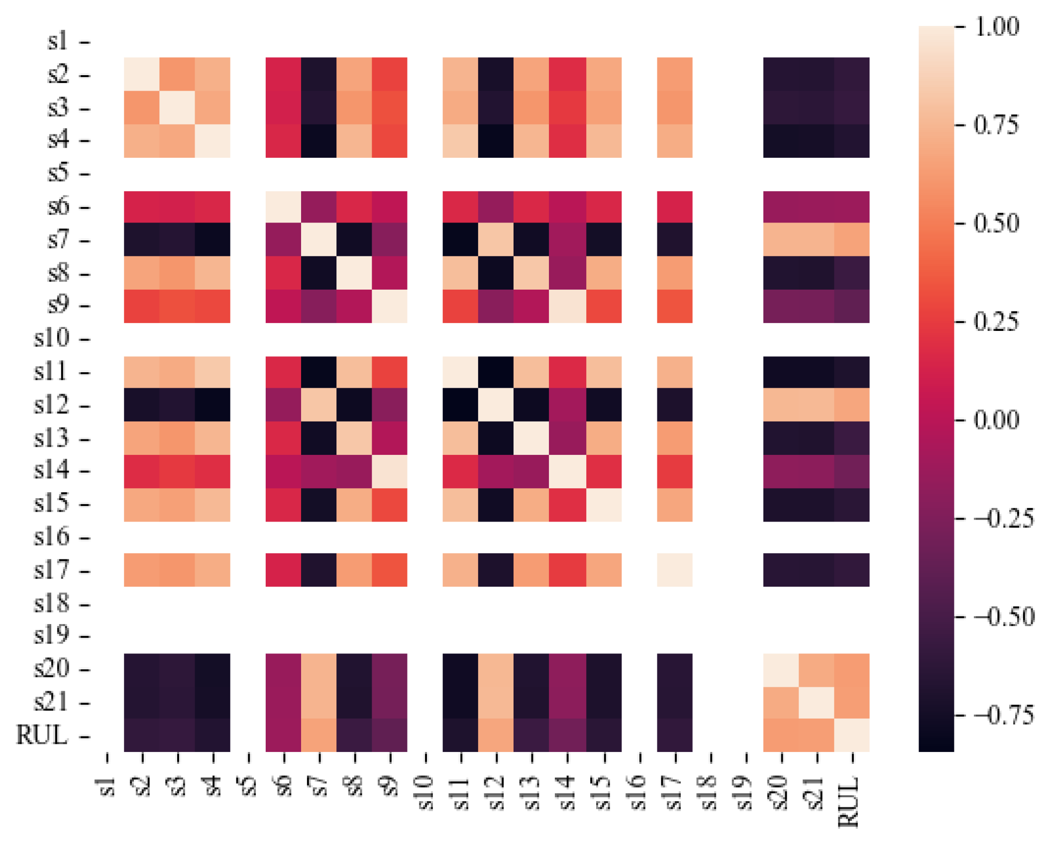
- Correlation analysis
3.3. Principal Component Analysis
3.4. Evaluation Metrics
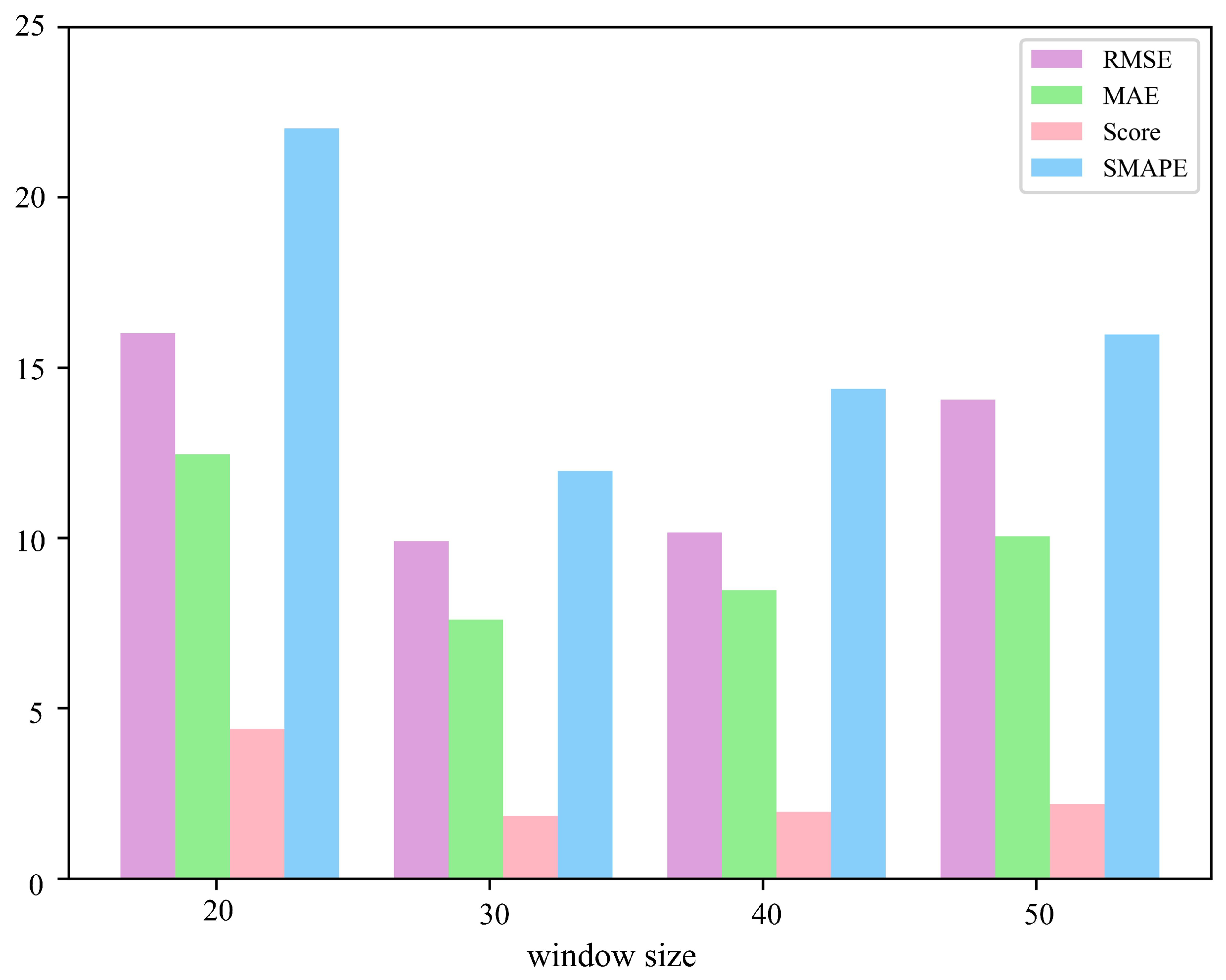
3.5. Experimental Results
4. Conclusions
Author Contributions
Funding
Institutional Review Board Statement
Informed Consent Statement
Data Availability Statement
Acknowledgments
Conflicts of Interest
References
- Che, C.; Wang, H.; Fu, Q.; Ni, X. Combining multiple deep learning algorithms for prognostic and health management of aircraft. Aerosp. Sci. Technol. 2019, 94, 105423. [Google Scholar] [CrossRef]
- Huang, Y.; Sun, G.; Tao, J.; Hu, Y.; Yuan, L. A modified fusion model-based/data-driven model for sensor fault diagnosis and performance degradation estimation of aero-engine. Meas. Sci. Technol. 2022, 33, 085105. [Google Scholar] [CrossRef]
- Volponi, A.J. Gas turbine engine health management: Past, present, and future trends. J. Eng. Gas Turbines Power 2014, 136, 051201-1. [Google Scholar] [CrossRef]
- Li, T.; Si, X.; Pei, H.; Sun, L. Data-model interactive prognosis for multi-sensor monitored stochastic degrading devices. Mech. Syst. Signal Process. 2022, 167, 108526. [Google Scholar] [CrossRef]
- Soualhi, A.; Lamraoui, M.; Elyousfi, B.; Razik, H. PHM survey: Implementation of prognostic methods for monitoring industrial systems. Energies 2022, 15, 6909. [Google Scholar] [CrossRef]
- Sadeghkouhestani, H.; Yi, X.; Qi, G.; Liu, X.; Wang, R.; Gao, Y.; Yu, X.; Liu, L. Prognosis and health management (PHM) of solid-state batteries: Perspectives, challenges, and opportunities. Energies 2022, 15, 6599. [Google Scholar] [CrossRef]
- Kong, Z.; Cui, Y.; Xia, Z.; Lv, H. Convolution and Long Short-Term Memory Hybrid Deep Neural Networks for Remaining Useful Life Prognostics. Appl. Sci. 2019, 9, 4156. [Google Scholar] [CrossRef] [Green Version]
- Huang, B.; Cohen, K.; Zhao, Q. Active anomaly detection in heterogeneous processes. IEEE Trans. Inf. Theory 2019, 65, 2284–2301. [Google Scholar] [CrossRef] [Green Version]
- Nguyen, V.; Seshadrinath, J.; Wang, D.; Nadarajan, S.; Vaiyapuri, V. Model-based diagnosis and RUL estimation of induction machines under interturn fault. IEEE Trans. Ind. Appl. 2017, 53, 2690–2701. [Google Scholar] [CrossRef]
- Wei, H.; Zhang, Q.; Gu, Y. Remaining useful life prediction of bearings based on self-attention mechanism, multi-scale dilated causal convolution, and temporal convolution network. Meas. Sci. Technol. 2023, 34, 045107. [Google Scholar] [CrossRef]
- Barraza-Barraza, D.; Tercero-Gomez, V.G.; Beruvides, M.G.; Limón-Robles, J. An adaptive ARX model to estimate the RUL of aluminum plates based on its crack growth. Mech. Syst. Signal Process. 2017, 82, 519–536. [Google Scholar] [CrossRef]
- Liu, Y.; Zuo, M.J.; Li, Y.F.; Huang, H.Z. Dynamic reliability assessment for multi-state systems utilizing system-level inspection data. IEEE Trans. Reliab. 2015, 64, 1278–1299. [Google Scholar] [CrossRef]
- Wang, C.; Lu, N.; Cheng, Y.; Jiang, B. A data-driven aero-engine degradation prognostic strategy. IEEE Trans. Cybern. 2021, 51, 1531–1541. [Google Scholar] [CrossRef] [PubMed]
- Zhao, H.; Liu, H.; Jin, Y.; Dang, X.; Deng, W. Feature extraction for data-driven remaining useful life prediction of rolling bearings. IEEE Trans. Instrum. Meas. 2021, 70, 1–10. [Google Scholar] [CrossRef]
- Qian, Y.; Yan, R.; Hu, S. Bearing degradation evaluation using recurrence quantification analysis and kalman filter. IEEE Trans. Instrum. Meas. 2014, 63, 2599–2610. [Google Scholar] [CrossRef]
- Wang, Z.; Wen, C.; Dong, Y. A method for rolling bearing fault diagnosis based on GSC-MDRNN with multi-dimensional input. Meas. Sci. Technol. 2023, 34, 055901. [Google Scholar] [CrossRef]
- Ren, L.; Zhao, L.; Hong, S.; Zhao, S.; Wang, H.; Zhang, L. Remaining useful life prediction for lithium-ion battery: A deep learning approach. IEEE Access 2018, 6, 50587–50598. [Google Scholar] [CrossRef]
- Wang, W.; Zhang, L.; Yu, H.; Yang, X.; Zhang, T.; Chen, S.; Liang, F.; Wang, H.; Lu, X.; Yang, S. et al. Early prediction of the health conditions for battery cathodes assisted by the fusion of feature signal analysis and deep-learning techniques. Batteries 2022, 8, 151. [Google Scholar] [CrossRef]
- Zhang, C.; Lim, P.; Qin, A.K.; Tan, K.C. Multiobjective deep belief networks ensemble for remaining useful life estimation in prognostics. IEEE Trans. Neural Netw. Learn. Syst. 2017, 28, 2306–2318. [Google Scholar] [CrossRef]
- Li, X.; Ding, Q.; Sun, J.Q. Remaining useful life estimation in prognostics using deep convolution neural networks. Reliab. Eng. Syst. Saf. 2018, 172, 1–11. [Google Scholar] [CrossRef] [Green Version]
- Liu, L.; Wang, L.; Yu, Z. Remaining useful life estimation of aircraft engines based on deep convolution neural network and LightGBM combination model. Int. J. Comput. Intell. Syst. 2021, 14, 165. [Google Scholar] [CrossRef]
- Kim, T.S.; Sohn, S. Multitask learning for health condition identification and remaining useful life prediction: Deep convolutional neural network approach. J. Intell. Manuf. 2021, 32, 2169–2179. [Google Scholar] [CrossRef]
- Liu, J.; Lei, F.; Pan, C.; Hu, D.; Zuo, H. Prediction of remaining useful life of multi-stage aero-engine based on clustering and LSTM fusion. Reliab. Eng. Syst. Saf. 2021, 214, 107807. [Google Scholar] [CrossRef]
- Xia, J.; Feng, Y.; Lu, C.; Fei, C.; Xue, X. LSTM-based multi-layer self-attention method for remaining useful life estimation of mechanical systems. Eng. Fail. Anal. 2021, 125, 105385. [Google Scholar] [CrossRef]
- Jin, R.; Chen, Z.; Wu, K.; Wu, M.; Li, X.; Yan, R. Bi-LSTM-based two-stream network for machine remaining useful life prediction. IEEE Trans. Instrum. Meas. 2022, 71, 1–10. [Google Scholar] [CrossRef]
- Li, X.; Jiang, H.; Liu, Y.; Wang, T.; Li, Z. An integrated deep multiscale feature fusion network for aeroengine remaining useful life prediction with multisensor data. Knowl.-Based Syst. 2022, 235, 107652. [Google Scholar] [CrossRef]
- Song, T.; Liu, C.; Wu, R.; Jin, Y.; Jiang, D. A hierarchical scheme for remaining useful life prediction with long short-term memory networks. Neurocomputing 2022, 487, 22–33. [Google Scholar] [CrossRef]
- Caceres, J.; Gonzalez, D.; Zhou, T.; Droguett, E.L. A probabilistic Bayesian recurrent neural network for remaining useful life prognostics considering epistemic and aleatory uncertainties. Struct. Control. Health Monit. 2022, 28, 1545–2255. [Google Scholar] [CrossRef]
- Kraus, M.; Feuerriegel, S. Forecasting remaining useful life: Interpretable deep learning approach via variational Bayesian inferences. Decis. Support Syst. 2019, 125, 113100. [Google Scholar] [CrossRef]
- Zu, T.; Kang, R.; Wen, M. Graduation formula: A new method to construct belief reliability distribution under epistemic uncertainty. J. Syst. Eng. Electron. 2020, 31, 626–633. [Google Scholar]
- Li, G.; Yang, L.; Lee, C.G.; Wang, X.; Rong, M. A Bayesian deep learning RUL framework integrating epistemic and aleatoric uncertainties. IEEE Trans. Ind. Electron. 2021, 68, 8829–8841. [Google Scholar] [CrossRef]
- Wang, C.; Miao, X.; Zhang, Q.; Bo, C.; Zhang, D.; He, W. Similarity-based probabilistic remaining useful life estimation for an aeroengine under variable operational conditions. Meas. Sci. Technol. 2022, 33, 114011. [Google Scholar] [CrossRef]
- Jiao, R.; Peng, K.; Dong, J. Remaining useful life prediction for a roller in a hot strip mill based on deep recurrent neural networks. IEEE/CAA J. Autom. Sin. 2021, 8, 1345–1354. [Google Scholar] [CrossRef]
- Long, B.; Wu, K.; Li, P.; Li, M. A novel remaining useful life prediction method for hydrogen fuel cells based on the gated recurrent unit neural network. Appl. Sci. 2021, 12, 432. [Google Scholar] [CrossRef]
- She, D.; Jia, M. A BiGRU method for remaining useful life prediction of machinery. Measurement 2021, 167, 108277. [Google Scholar] [CrossRef]
- Zaidan, M.A.; Mills, A.R.; Harrison, R.F.; Fleming, P.J. Gas turbine engine prognostics using Bayesian hierarchical models: A variational approach. Mech. Syst. Signal Process. 2016, 71, 120–140. [Google Scholar] [CrossRef]
- Pei, H.; Si, X.; Hu, C.; Li, T.; He, C.; Pang, Z. Bayesian deep-learning-based prognostic model for equipment without label data related to lifetime. IEEE Trans. Syst. Man Cybern. Syst. 2023, 53, 504–517. [Google Scholar] [CrossRef]
- Gao, Z.; Tao, J.; Su, Y.; Zhou, D.; Zeng, X.; Li, X. Efficient rare failure analysis over multiple corners via correlated Bayesian inference. IEEE Trans. Comput.-Aided Des. Integr. Circuits Syst. 2020, 39, 2029–2041. [Google Scholar] [CrossRef]
- Ping, G.; Chen, J.; Pan, T.; Pan, J. Degradation feature extraction using multi-source monitoring data via logarithmic normal distribution based variational auto-encoder. Comput. Ind. 2019, 109, 72–82. [Google Scholar] [CrossRef]
- Arias Chao, M.; Kulkarni, C.; Goebel, K.; Fink, O. Aircraft Engine Run-to-Failure Dataset Under Real Flight Conditions for Prognostics and Diagnostics. Data 2021, 6, 5. [Google Scholar] [CrossRef]


| Index | Symbol | Description | Units |
|---|---|---|---|
| 1 | T2 | Total temperature at fan inlet | R |
| 2 | T24 | Total temperature at LPC outlet | R |
| 3 | T30 | Total temperature at HPC outlet | R |
| 4 | T50 | Total temperature at LPT outlet | R |
| 5 | P2 | Pressure at fan inlet | psia |
| 6 | P15 | Total pressure in bypass-duct | psia |
| 7 | P30 | Total pressure at HPC outlet | psia |
| 8 | Nf | Physical fan speed | rpm |
| 9 | Nc | Physical core speed | rpm |
| 10 | epr | Engine pressure ratio (P50/P2) | - |
| 11 | Ps30 | Static pressure at HPC outlet | psia |
| 12 | phi | Ratio of fuel flow to Ps30 | pps/psi |
| 13 | NRf | Corrected fan speed | rpm |
| 14 | NRc | Corrected core speed | rpm |
| 15 | BPR | Bypass ratio | - |
| 16 | farB | Burner fuel–air ratio | - |
| 17 | htBleed | Bleed enthalpy | - |
| 18 | Nf_dmd | Demanded fan speed | rpm |
| 19 | PCNfR_dmd | Demanded corrected fan speed | rpm |
| 20 | W31 | HPT coolant bleed | lbm/s |
| 21 | W32 | LPT coolant bleed | lbm/s |
| RMSE | MAE | Score | SMAPE (%) | |
|---|---|---|---|---|
| BMLP | 37.90 | 35.09 | 22.34 | 38.80 |
| BLSTM | 25.13 | 20.08 | 9.05 | 23.16 |
| BGRU | 24.58 | 19.49 | 8.33 | 22.07 |
| BBiLSTM | 11.04 | 10.30 | 3.02 | 13.23 |
| BiGRU-IVBI | 9.91 | 7.60 | 1.84 | 11.96 |
| BiGRU-IVBI (non-PCA) | 11.47 | 9.43 | 2.75 | 13.86 |
| Methods and References | RMSE |
|---|---|
| MODBNE [19] | 17.96 |
| DCNN [20] | 12.61 |
| LightGBM [21] | 12.79 |
| MT-CNN [22] | 12.48 |
| MLSA [24] | 11.57 |
| BiLSTM [25] | 11.96 |
| IDMFFN [26] | 12.18 |
| LSTM [27] | 11.80 |
| BiGRU-IVBI | 9.91 |
| Window Size | RMSE | MAE | Score | SMAPE (%) |
|---|---|---|---|---|
| 20 | 16.00 | 12.46 | 4.39 | 22.02 |
| 30 | 9.91 | 7.60 | 1.84 | 11.96 |
| 40 | 10.16 | 8.47 | 1.96 | 14.37 |
| 50 | 14.06 | 10.05 | 2.19 | 15.97 |
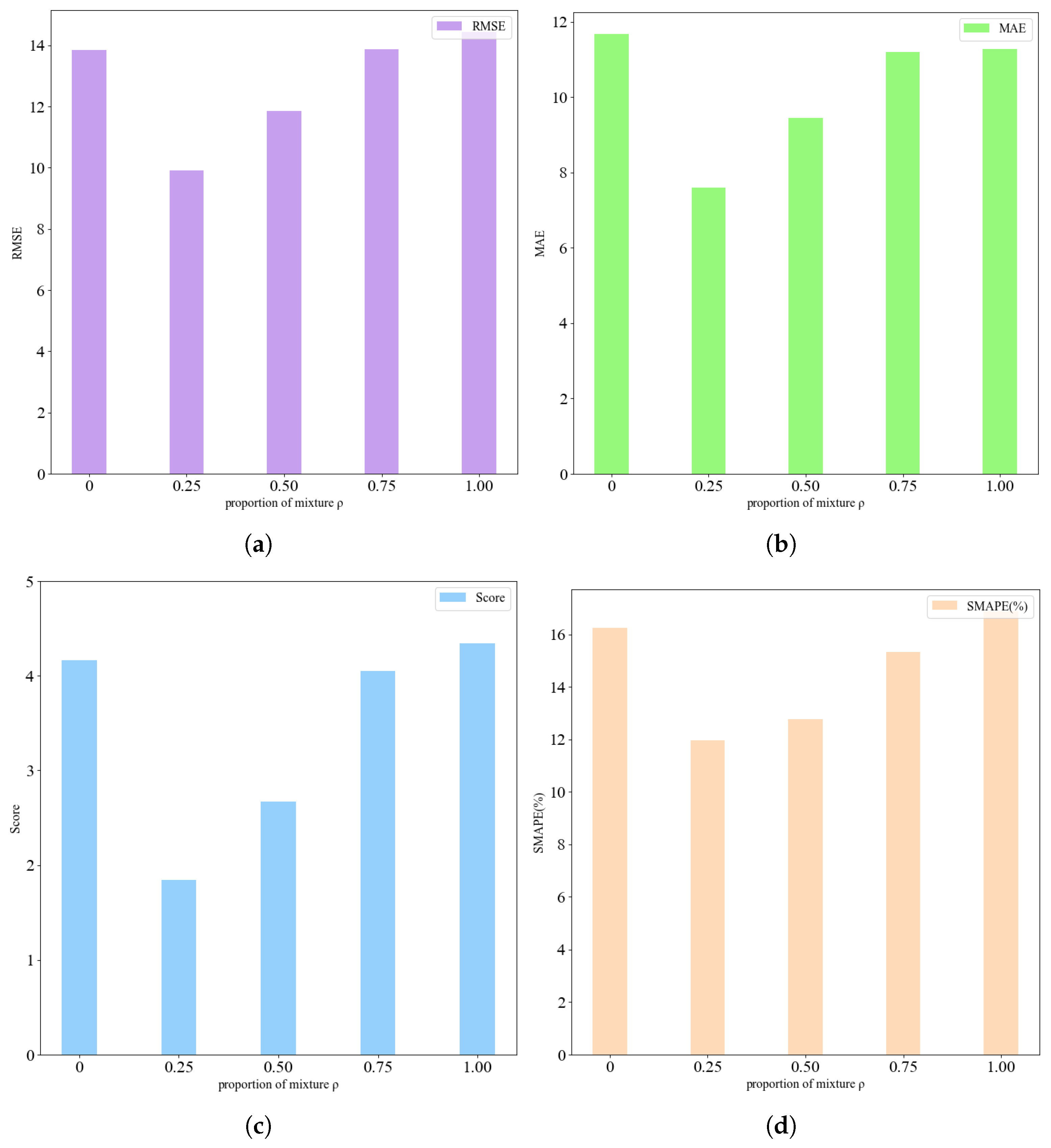
| Model | RMSE | MAE | Score | SMAPE (%) |
|---|---|---|---|---|
| = 0 | 13.85 | 11.67 | 4.16 | 16.25 |
| = 0.25 | 9.91 | 7.60 | 1.84 | 11.96 |
| = 0.50 | 11.85 | 9.44 | 2.67 | 12.76 |
| = 0.75 | 13.88 | 11.19 | 4.05 | 15.34 |
| = 1.00 | 14.43 | 11.27 | 4.34 | 16.87 |
Disclaimer/Publisher’s Note: The statements, opinions and data contained in all publications are solely those of the individual author(s) and contributor(s) and not of MDPI and/or the editor(s). MDPI and/or the editor(s) disclaim responsibility for any injury to people or property resulting from any ideas, methods, instructions or products referred to in the content. |
© 2023 by the authors. Licensee MDPI, Basel, Switzerland. This article is an open access article distributed under the terms and conditions of the Creative Commons Attribution (CC BY) license (https://creativecommons.org/licenses/by/4.0/).
Share and Cite
Hu, Y.; Bai, Y.; Fu, E.; Liu, P. A Novel Remaining Useful Life Probability Prediction Approach for Aero-Engine with Improved Bayesian Uncertainty Estimation Based on Degradation Data. Appl. Sci. 2023, 13, 9194. https://doi.org/10.3390/app13169194
Hu Y, Bai Y, Fu E, Liu P. A Novel Remaining Useful Life Probability Prediction Approach for Aero-Engine with Improved Bayesian Uncertainty Estimation Based on Degradation Data. Applied Sciences. 2023; 13(16):9194. https://doi.org/10.3390/app13169194
Chicago/Turabian StyleHu, Yanyan, Yating Bai, En Fu, and Pengpeng Liu. 2023. "A Novel Remaining Useful Life Probability Prediction Approach for Aero-Engine with Improved Bayesian Uncertainty Estimation Based on Degradation Data" Applied Sciences 13, no. 16: 9194. https://doi.org/10.3390/app13169194