Abstract
To study the influence law of the seismic response of underground station structures at liquifiable interlayer sites, a two-dimensional numerical model of the interaction between the soil and station structure was established based on the finite difference software FLAC3D. The nonlinear dynamic response of the station structure located at the liquifiable interlayer site was analyzed considering the location distribution, relative density, and thickness of the liquifiable interlayer. The results show that the deformation of the structure is greatest when the liquifiable interlayer is distributed on both sides of the station side walls, while the interlayer has an energy-dissipating and damping effect on the upper station structure when it is located at the bottom of the structure. The lower the relative density of the liquifiable interlayer is, the stronger the internal dynamic response of the structure will be, and the more unfavorable it will be to the seismic resistance of the structure. When the liquefiable interlayer is only present in the lateral foundation of the station, an increase in its thickness results in a stronger shear effect on the structure and a higher probability of damage. However, when the thickness of the liquifiable interlayer reaches a point where the entire station is placed within it, the lateral force and deformation of the structure are significantly reduced.
1. Introduction
Large-scale transportation construction will inevitably result in underground space structures crossing liquefiable soils. When an earthquake occurs, the liquefiable soil will “liquefy” under the vibration load, causing the site soil to lose its bearing capacity and assume a liquid state. The liquefaction of the site soil will have an important impact on the underground structure [1,2]. For example, the 1995 Hanshin earthquake in Japan caused the devastating collapse of the Daikai subway station. The investigation found that extreme liquefaction occurred at both the coastal backfill site and in the artificial island area, causing widespread, permanent deformation of the foundation in the horizontal direction [3,4,5]. In the 2008 Wenchuan earthquake in Sichuan, the phenomenon of foundation liquefaction occurred in specific areas with severe earthquake damage, and underground structures such as tunnels were damaged to varying degrees [6,7]. In the 2011 earthquake off the Pacific Ocean in Japan, soil liquefaction occurred in a large region of coastal areas, many buildings were subjected to serious foundation subsidence, and some shallowly buried underground structures even appeared to rise above the ground [8,9]. Therefore, it is of great practical importance to study the seismic performance of underground structures at liquefiable sites.
In recent years, scholars in related fields have successively studied the seismic response law of underground station structures in liquefiable strata. Chen et al. [10] conducted a series of shaking table experimental studies on irregular cross-section subway underground structures at liquefiable sites and provided a specific description of the liquefaction development law of foundations and the damage mechanism of station structures. Zhuang et al. [11] revealed the seismic response characteristics of underground station structures in slightly inclined liquefiable foundations through shaking table tests and further compared and analyzed the effect of ground inclination changes on station structures in liquefiable sites. Ding et al. [12] conducted a series of shaking table tests to reveal the effect of groundwater level changes on the degree of soil liquefaction and the seismic response pattern of underground structures. In addition to the methods employed through model tests, many scholars have used numerical simulations to investigate the dynamic response characteristics of subsurface structures at liquefiable sites [13,14,15,16,17,18]. Bao et al. [13] interpreted the seismic performance and uplift mechanism of large subway station structures in liquefiable soils considering the excavation process during the construction of the structure. Hu et al. [14,15] used the numerical analysis method coupled with the finite element and finite difference method to analyze the dynamics of rectangular structures in saturated sandy soil sites and explored the influences of different relative densities of sandy soils on the seismic response and uplift effect of underground structures. Tian et al. [16] explored the force and deformation mechanism of an underground corridor structure at a non-homogeneous liquefiable site and further investigated the effect of burial depth on the dynamic response of the structure.
In the above studies, the foundations were mostly considered as homogeneous liquefiable sites, or the station structures were wholly placed in liquefiable layers. The seismic response characteristics of station structures in non-homogeneous layered liquefiable sites need to be investigated further. Shen et al. [17] and Chen et al. [18] showed that underground structures undergo much more seismic damage at laminated liquefiable sites than at homogeneous liquefiable sites. In engineering practice, liquefiable foundations are mostly present in the form of liquefiable interlayers. The existing research is not explicit with respect to the influence law of liquefiable interlayers on the seismic response of underground station structures. In view of this, we take the liquefiable interlayer site as our research object, integrate the influences of the spatial location distribution, relative density and thickness of the liquefiable interlayer on the structure of a subway station under earthquake action, and draw some practical conclusions for seismic stability analysis in similar projects.
2. Numerical Calculation Method
2.1. Geometric Model and Site Condition Setting
A typical subway station is a two-story, three-span structure. The cross-sectional dimensions of the main part are shown in Figure 1. The top plate of the station structure is buried at a depth of 5 m, the width of the structural model is 21.34 m, the height is 14.89 m, the size of the central column of the station structure is 0.6 m × 1.1 m, and the distance between the longitudinal columns of the central column is 9.12 m.
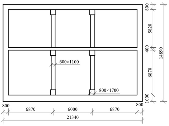
Figure 1.
Standard cross-section of station structure (unit: mm).
In this study, seven different site conditions were constructed, and three sets of numerical models were set up for comparison and analysis according to different variables. The influence of the location of the liquefiable interlayer on the dynamic response of the structure was investigated in cases a, b, and c; the influence of the relative density of the interlayer was investigated in cases b, d, and e; and the influence of the thickness of the interlayer was investigated in cases b, f, and g. The water level is assumed to be at the ground surface in each model, and the liquefiable interlayer is a sandy soil, while the rest of the site soil is non-liquefiable clay. A simplified model of the soil–station structure and the arrangement of the monitoring points are shown in Figure 2. The variable D is the burial depth at the top of the liquefiable interlayer, and H is the thickness of the interlayer. The distribution of the soil layers in each case is shown in Table 1.
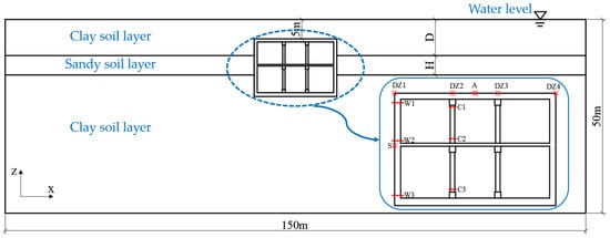
Figure 2.
Soil layer distribution and monitoring point layout of the site.

Table 1.
Distribution of the liquefiable interlayer in each case.
2.2. Numerical Model Establishment and Parameter Setting
The Finn model was proposed by Martin et al. [19] to solve the problem of volume strain and the pressure change pattern of soil under cyclic loading based on experiments. This model introduces the pore pressure rise model into the Mohr–Coulomb model, which can simulate the process of accumulation and development of super-pore water pressure in soil under dynamic loading until the point of liquefaction. Byrne [20] summarized and analyzed the test data of Martin et al. to simplify the Finn model, and the derived strain increment calculation equation is shown in Formula (1):
where is the shear strain, is the volume strain, and is the volume strain increment.
In Formula (1), C1 and C2 are the constant related to the relative density of the sandy soil and the corrected slamming number, which is calculated empirically using the following formula:
Many scholars [21,22,23] have chosen the Finn model to describe the liquefaction behavior of soil and obtained satisfactory data results, which shows that the Finn model is an appropriate tool for investigating the liquefaction principal of soil in this paper.
In order to improve computational accuracy in numerical analysis, interface elements are usually added between the soil and the structure in order to more realistically simulate the nonlinear contact phenomena between the structure and the soil. Empirically, the normal stiffness kn and shear stiffness ks, the key parameters of the contact surface interface, can be taken as 10 times the equivalent stiffness of the surrounding “hardest” adjacent area [24], as shown in Formula (5). The internal friction angle can be approximated as roughly 0.5 times that of the surrounding soil layer:
where K is the bulk modulus, G is the shear modulus, and is the minimum size of the connection area in the normal direction of the contact surface.
Based on the finite difference software FLAC3D, a numerical model of the interaction between the soil layer and the station structure was established. In order to eliminate the influence of the model boundary effect as much as possible, the calculation range of the foundation is taken as 7 times the length of the station structure, being 150 m in the horizontal direction with a 50 m depth below the ground surface in the vertical direction. The elastic constitutive model is used for concrete, and the Mohr–Coulomb strength criterion is followed for site soils. During the seepage analysis, the soil elements were set up as isotropic models, and the station structure elements were set up as impermeable models. The Byrne-simplified Finn pore pressure model is used to simulate the liquefaction behavior of liquifiable interbedded site soils under seismic action due to the rise in pore water pressure. The physical and mechanical parameters of each stratum soil are given in Table 2, with reference to our engineering experience.
Table 2.
Material parameters used in numerical analysis.
The station is a cast-in-place reinforced concrete structure with a concrete grade of C40, and solid elements are used to model it. To improve the computational efficiency, the numerical model is simplified to a two-dimensional plane strain model considering the interaction between the soil and structure, and the continuity of the central column is considered in light of the equivalent discount of stiffness, which is equated to a continuous longitudinal wall with a thickness of 0.6 m. The interface element is set to simulate the interaction between the soil and the underground station structure. The specific physical and mechanical parameters of the station structure and the interface element parameters are shown in Table 2. The mesh division of the numerical model of the soil–subway station structure for case b is shown in Figure 3.
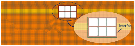
Figure 3.
Schematic diagram of numerical model meshing.
2.3. Material Damping Selection
Considering the calculation accuracy and time cost, we used local damping to reflect the nonlinear characteristics of soil materials and the energy loss of the soil–station structure interaction model in the dynamic analysis process. According to our engineering experience and previous research [25,26], the critical damping ratio of rock and soil materials was taken as 10%, and the critical damping ratio of reinforced concrete materials was taken as 5%.
For the sandy soil interlayer, the hysteresis effect due to soil liquefaction needs to be considered further in the dynamic calculation process. Since hysteresis damping can be employed simultaneously with other types of damping and does not affect the calculation time step, hysteresis damping was further applied to the sandy soil interlayer to characterize its hysteresis properties. Among the various models, the Hardin–Drnevich model requires only one parameter for the reference strain, and the fitted equation for the normalized cut-line modulus () is shown in Formula (6):
For sandy soil materials, the reference strain is generally taken as 0.06. The modulus decay curves derived from the hysteresis damping model selected for this paper were compared with the experimental data of Seed et al. [27], and the results are shown in Figure 4. It can be seen that the modulus decay curves fitted using the Hardin–Drnevich model are closer to the measured data.
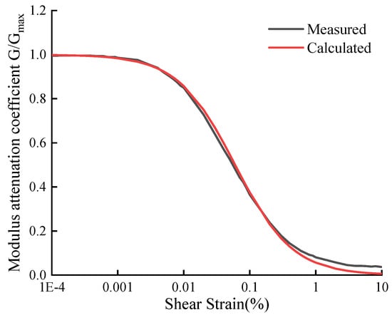
Figure 4.
Shear modulus reduction curve for sand compared with Seed and Idriss (1970) [27].
2.4. Boundary Conditions and Ground Vibration Input
In the process of static analysis, fixed displacement constraint is used at the bottom of the model and in the longitudinal direction, the boundary on both sides is set as a normal displacement constraint, and the ground surface is a free boundary [28]. The initial stress field is obtained after static equilibrium. Then, a natural water level condition is imposed on the ground surface, the bottom and both sides of the model are set as impermeable boundaries, and fluid parameters are established to obtain a constant seepage field. When performing the static analysis, the effects of construction and other factors are ignored, and the ground loads on the underground structure are not considered.
As the bottom element of the model in this numerical analysis model is soft clay, the acceleration time course and velocity time course cannot be applied directly. It is necessary to convert the acceleration and velocity into a stress timescale and then apply them to the bottom of the model. The specific conversion equation [24] is shown in Formula (7):
where represents the shear components of the velocity at the boundary, is the mass density, and represents the s-wave velocities.
Therefore, in the process of dynamic analysis, the existing static constraints at the bottom of the model are first removed, and static boundary conditions are applied at the bottom of the model. Then, the seismic load is applied, and the free field boundary is applied on both sides of the model to reduce the reflection of seismic waves at the model boundary [29,30].
The seismic wave used in this study was the Kobe wave, which is a typical seismic wave measured in structural seismic studies, with an original peak acceleration of 0.85 g in the north–south direction and a duration of the strong seismic part of approximately 7 s. In order to fully reflect the characteristics of site liquefaction, the original peak acceleration of ground shaking is amplitude modulated. The peak acceleration of ground shaking is 0.2 g after amplitude modulation, and the input ground shaking holding time is 20 s. The seismic wave acceleration time curve and Fourier spectrum are shown in Figure 5. To ensure the computational speed and accuracy of the numerical simulation, the amplitude-modulated seismic wave is passed through the fast Fourier transform (FFT) to obtain the input ground shaking power spectrum, the high-frequency components larger than 5 Hz are filtered out through filtering, and then the filtered seismic wave is baseline-corrected. The filtered and baseline-corrected seismic waves are input from the bottom of the model in a stress-time-dependent manner.
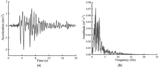
Figure 5.
Time history and Fourier spectrum of earthquake acceleration. (a) Acceleration time history curve; (b) Fourier spectra of acceleration.
3. Liquefaction Distribution Characteristics
In the numerical calculation process, the excess pore pressure ratio (EPPR) is used to represent the liquefaction degree of the soil [24], which is defined as shown in Formula (8):
where is the average effective stress of the element during the dynamic calculation, and is the average effective stress of the element before the dynamic calculation.
In order to reflect the distribution characteristics of liquefaction zones of liquefiable interlayer sites under different influencing factors, the EPPR clouds of the sandy interlayer after the end of seismic action in different cases are given in Figure 6. When the EPPR is greater than 0.7, the site is considered to be initially liquefied, and when the EPPR is equal to 1, the site is considered to be completely liquefied.
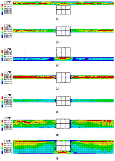
Figure 6.
Distribution cloud map of excess pore pressure ratio of liquefied interlayer after the end of the earthquake in different conditions: (a) case a (H = 5 m, Dr = 50%), (b) case b (H = 5 m, Dr = 50%), (c) case c (H = 5 m, Dr = 50%), (d) case d (H = 5 m, Dr = 30%), (e) case e (H = 5 m, Dr = 70%), (f) case f (H = 12 m, Dr = 50%), (g) case g (H = 20 m, Dr = 50%).
From Figure 6, it can be seen that the liquefaction range of the liquefiable interlayer in each case is basically symmetrically distributed, and the soil near the side wall of the station structure does not liquefy. The reason for this is that the stiffness difference between the station structure and the liquefiable soil layer is too large, and the excess pore water pressure of the soil near the side wall cannot easily accumulate and develop. In case a, when the liquefiable interlayer is located in the upper part of the structure, partial liquefaction occurs in the middle part of the shallow sandy soil on the surface. In case d, when the relative density of the sand interlayer is 30%, almost all the soil in the liquefiable interlayer is liquefied, except for that near the side wall of the structure, and no liquefaction occurs in the liquefiable interlayer in case e, which has the highest relative density. In both case c and case g, liquefaction occurs at the bottom of the structure because the average effective stress at the bottom of the structure is much lower than that at other locations at the same depth due to the presence of the station structure, and liquefaction is more likely to be triggered by the seismic action. In both case b and case f, liquefaction only occurs at the two ends of the negative level of the structure, away from the side walls. In summary, the liquefaction of the liquefiable layer is most significant in cases d and g, which will have an important impact on the station structure and should be taken into account in the analysis.
4. Dynamic Response Analysis of Station Structure
4.1. Influence of the Relative Position of the Liquifiable Interlayer
Element A, in the middle of the top plate of the structure, was monitored, and the acceleration time course in each case was obtained as shown in Figure 7. It can be seen from the figure that the peak acceleration of the top plate of the station is the greatest when the liquifiable interlayer is located on both sides of the station (case b). When the liquifiable interlayer is located at the bottom of the station structure (case c), the peak acceleration of the structure is the lowest, because the soil under the structure is liquefied under the seismic load, and the soil loses its shear characteristics and hinders the transmission of shear waves. Accordingly, the disturbance of the upper metro station is greatly reduced. This indicates that when the liquifiable interlayer is distributed in the lower area of the station, it has a certain seismic isolation effect on the station structure.
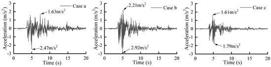
Figure 7.
Time course curves of station roof acceleration under different spatial location distribution conditions of the liquefaction sandwich.
The time course curves of the relative horizontal displacement of the top and bottom of the structure when the liquifiable interlayer is located in different spatial positions are given in Figure 8. As can be seen in the figure, the peak relative displacement at the top and bottom of the structure is greatly influenced by the distribution of the liquifiable interlayer location. The peak relative displacement of the structure is the greatest in case b, where the liquifiable interlayer crosses the side wall of the station structure, and the maximum relative displacement is 28.08 mm. Meanwhile, in case c, when the liquifiable interlayer is located at the bottom of the structure, the peak relative displacement is only 12.12 mm, which is reduced by 56.8% compared with case b. From the point of view of structural seismic resistance, when the liquifiable interlayer is located in the lateral foundation of the station structure, the lateral deformation of the structure is the greatest, and it is more likely to be damaged under the earthquake action.
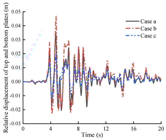
Figure 8.
Influence of the spatial position distribution of the liquifiable interlayer on the relative displacement of the top and bottom plates of the station structure.
The underground structure is constrained by the surrounding soil layer and mainly undergoes shear deformation under the action of the earthquake. To further investigate the influence of the degree of liquefaction of the interlayer on the structural forces, stress monitoring was conducted, focusing on the key parts of the wall–column structure, and the maximum shear stress at each monitoring point of the structure was obtained as shown in Figure 9. After comparison, it can be seen that the shear stresses at various parts of the structure are higher when the liquifiable interlayer crosses the side wall of the structure (case b), and the shear stresses at the W2 section of the side wall are especially prominent. When the liquifiable interlayer is located at the bottom of the structure (case c), the magnitude of the shear stresses at all parts of the structure is reduced, which also proves that the interlayer has a certain seismic isolation effect when it is located at the bottom of the structure from the perspective of force.
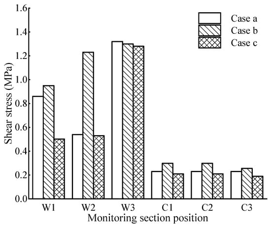
Figure 9.
Influence of the spatial position distribution of the liquifiable interlayer on the shear stress at each section position.
4.2. Influence of the Relative Density of the Liquifiable Interlayer
Relative density has an important influence in triggering sand liquefaction. In this section, the most unfavorable case (case b) of the liquifiable interlayer crossing the station structure analyzed in the previous section is used as the base case, and the relative position and thickness of the liquifiable interlayer are kept constant to further investigate the effect of the variation in the relative density of the sand interlayer on the dynamic response of the station structure.
Figure 10 shows the acceleration amplification effect of the station structure plate and column. On the whole, the acceleration response of the station structure at different heights differs under the seismic effect, and the peak acceleration of the plate structure is much lower than the peak acceleration of the column structure. The lower the relative density of the sand interlayer is, the stronger the acceleration amplification effect inside the structure will be. The acceleration response at the top and bottom plates of the structure is less affected by the relative density, while the acceleration of the middle plate and the middle column structure is strongly affected by the change in the relative density of the sand interlayer. It is worth noting that the maximum acceleration amplification coefficient of the column structure on the upper level of the station reaches 6.45 in case d. The reason for this is that the great liquefaction of the sandwich soil leads to the weakening of the restraint effect of the soil on the structure, which results in greater differential acceleration inside the structure [31,32].
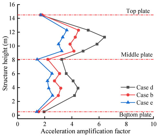
Figure 10.
Acceleration amplification effect of the station plate and column structure.
Figure 11 shows the maximum horizontal relative displacement curves of the station side walls under different relative densities of the interlayer. From the figure, it can be seen that the horizontal relative displacement of the structure, with a 70% relative density of the interlayer, is the lowest in case e. As the relative density of the sand interlayer decreases, the degree of liquefaction gradually increases, and the horizontal deformation of the station structure side wall also gradually increases. The maximum relative displacement between the top and bottom plates is 33.4 mm in case d, which increases by 29.4% compared with case e.
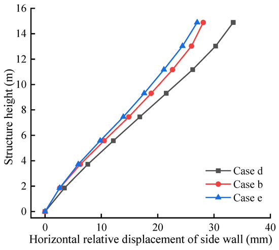
Figure 11.
Influence of the relative density of the liquifiable interlayer on the horizontal relative displacement of the side wall.
Figure 12 shows the maximum shear stress at each measured point of the station structure under different relative densities of the liquifiable interlayer. From the figure, it can be seen that the maximum shear stress magnitude at each key section of the wall and column decreases with the increase in the relative density of the sand interlayer, but the degree of reduction varies between different section locations. The shear stress at the bottom of the station structure is less affected by the relative density. The shear stress at the connection between the side wall and the middle plate decreases most significantly with the increase in the relative density and is most affected by the degree of liquefaction of the sand interlayer, which should be given more consideration in seismic design.
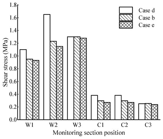
Figure 12.
Influence of the relative density of the liquifiable interlayer on the shear stress at each section.
Figure 13 shows the time course curve of the soil and water compressive stress in the middle of the side-wall-monitoring element S. It can be seen that the development trend of the soil and water compressive stress is similar in each case, always progressing through the three stages of “smooth development, fluctuating rise and stabilization”. The lateral wall soil and water compressive stresses show a decreasing trend with the increase in the relative density of the sand and soil interlayer, and the lower the relative density is, the greater the peak soil and water compressive stresses in the lateral wall are. Because the relative density of the sandwich soil decreases, the degree of liquefaction increases, the development of super-pore water pressure is more significant, and the soil and water compressive stress on the side wall increases, which further increases the influence of horizontal shear on the side wall.
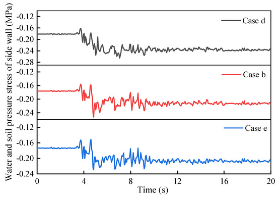
Figure 13.
Time history curve of dynamic water and soil compressive stress on the side wall.
4.3. Influence of the Layer Thickness of the Liquifiable Interlayer
The analysis in this section, again, takes case b as the benchmark case, keeps the relative position and relative density of the liquifiable interlayer unchanged, gradually increases the thickness of the sand layer, and further explores the influence of the thickness change in the liquifiable interlayer on the dynamic response of the station structure.
Figure 14 shows the maximum horizontal displacement curve of the side wall of the station under different layer thicknesses of the liquifiable interlayer. It can be seen from the figure that when the whole liquifiable interlayer is only distributed in the lateral foundation of the structure (case b and case f), as the thickness of the interlayer increases, the horizontal relative displacement amplitude of the side walls gradually increases, and the lateral deformation of the structure also increases. When the thickness of the liquifiable layer is 12 m (case f), the relative displacement between the top and bottom of the structure is the greatest, reaching 46.6 mm, which is 1.6 times that of the site where the interlayer thickness is 5 m. In case g, when the thickness of the liquifiable layer is 20 m, the station structure is completely placed in the liquefiable interlayer, and the relative displacement of the side wall of the structure is the lowest, only 26.5 mm. Under earthquake action, the water and soil pressure produced by the liquefiable sand interlayer on the structure is greater than that of the non-liquefiable clay layer. As the thickness of the liquefiable layer increases, the contact area between the side wall of the station and the liquefiable interlayer increases, further increasing the lateral deformation of the structure; When the structure is completely placed in the liquefiable layer, the water and soil pressure difference on the structure is greatly reduced, so the deformation of the structure is minimal.
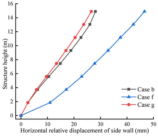
Figure 14.
Influence of layer thickness of liquifiable interlayer on horizontal relative displacement of side wall.
The shear stresses in each key part of the structure under different thicknesses of liquefaction interlayer are shown in Figure 15. From the figure, it can be seen that when all the liquifiable interlayer is only located in the lateral foundation of the structure (case b and case f), the influence law of the liquifiable layer thickness on each part of the station structure is not consistent. The variation of liquifiable interlayer thickness does not have much effect on the magnitude of shear stress in each section of the central column, the shear stress at the intersection of the structural side wall and the top and bottom plate gradually increases with the increase in the interlayer thickness, but the magnitude of the shear stress at the connection between the side wall and the central plate gradually decreases. When the thickness of the liquifiable interlayer is as great as 20 m (case g), the amplitude of the shear stress in all parts of the station wall and column structure is the lowest, being much lower than in other cases. The reason for this phenomenon is that the soil in the lower part of the structure liquefies first, and the soil near the sides of the side walls flows downward, which slows down the effect on the horizontal shear of the structure.
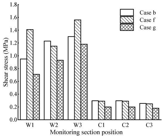
Figure 15.
Influence of the layer thickness of the liquifiable interlayer on the shear stress at each section position.
The research of Xia et al. [33] showed that the thickness of the liquifiable soil layer is one of the key factors affecting the uplift of underground structures. Firstly, the developmental trend of the vertical displacement of the structure is analyzed. Taking case b as an example, it can be seen from Figure 16 that the structure gradually starts to float within 0~4 s, and the floating amplitude is almost negligible. With the increase in seismic intensity, the vertical displacement of each monitoring point climbs rapidly for around 4 s and then reaches the peak and fluctuates; at the end of the seismic action, the vertical displacement tends to become stable and remains basically unchanged.
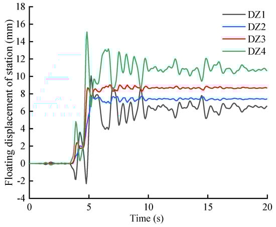
Figure 16.
Time–history curve of the floating displacement of the station structure in case b.
To further investigate the uplift response of the station structure under different liquifiable interlayer thicknesses, the final uplift displacement values of the structure under different layer thicknesses of the liquifiable interlayer are given in Figure 17. It can be seen that the floating displacement of the station structure increases with the increase in the thickness of the liquifiable interlayer, and there is a clear difference in the floating phenomenon. The specific performance is such that the floating displacement on the left side is lower than that on the right. When the station structure is wholly placed in the liquifiable layer (case g), the degree of floating is the greatest. Although the shearing effect on the structure in the horizontal direction is weakened at this time, the adverse effect on the structure due to the floating effect still needs to be considered in the seismic design.
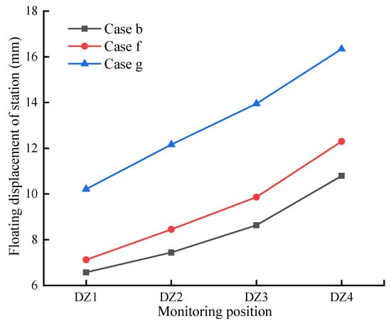
Figure 17.
Influence of liquifiable interlayer layer thickness on the uplifting displacement of the station.
5. Conclusions
Based on the finite difference numerical calculation method, the influence law of the liquifiable interlayer on the dynamic response of underground station structures was analyzed, and the influences of interlayer location distribution, relative density, and layer thickness on structural force deformation were explored. The main conclusions are as follows:
- (1)
- The liquefaction range of the liquefiable interlayer is basically symmetrically distributed, and the liquefied area is mainly distributed at the bottom of the station structure and on both sides, away from the structure area. When the wall stiffness is great compared with the surrounding soil, the site soil near the structural side wall cannot easily liquefy.
- (2)
- The relative location distribution of the liquifiable interlayer has a strong influence on the structural seismic response. When the liquifiable interlayer crosses the middle of the station, the shear stress and lateral deformation of the structure are the greatest, while when the liquifiable interlayer is located in the bottom area of the station structure, the dynamic response of the station structure is greatly reduced, and at this time, the liquifiable interlayer has certain effects of seismic damping and seismic isolation, which are beneficial in supporting the seismic resistance of the station structure to a certain extent.
- (3)
- When the liquifiable interlayer is distributed in the middle of the lateral foundation of the station structure, the shear stress of the negative one-story wall and column decreases with increasing relative density, and the structural shear stress of the wall column near the bottom plate is not greatly affected by the relative density. When the relative density of the sand interlayer is low, the internal acceleration response of the structure is strong, and the acceleration amplification effect of the middle column structure is especially prominent.
- (4)
- When the whole liquifiable interlayer is only located in the lateral foundation of the structure, with an increase in the thickness of the interlayer, the shearing effect on the station structure under the earthquake action becomes stronger, and the probability of damage becomes greater. However, when the thickness of the liquifiable layer increases to a certain extent, the station structure is wholly placed in the liquifiable interlayer, and although the horizontal disturbance of the structure decreases at this time, the uplift displacement of the structure reaches its maximum.
Author Contributions
Writing—original draft preparation, J.Y.; writing—review and editing, Y.L. and J.Y. All authors have read and agreed to the published version of the manuscript.
Funding
This research received no external funding.
Institutional Review Board Statement
Not applicable.
Informed Consent Statement
Not applicable.
Data Availability Statement
The data are contained within the present article. The other data presented in this research are available in [27].
Conflicts of Interest
The authors declare no conflict of interest.
References
- Zhuang, H.; Chen, G.; Hu, Z.; Qi, C. Influence of Soil Liquefaction on the Seismic Response of a Subway Station in Model Tests. Bull. Eng. Geol. Environ. 2016, 75, 1169–1182. [Google Scholar] [CrossRef]
- Boulanger, R.W.; Kamai, R.; Ziotopoulou, K. Liquefaction induced strength loss and deformation: Simulation and design. Bull. Earthq. Eng. 2014, 12, 1107–1128. [Google Scholar] [CrossRef]
- Uenishi, K.; Sakurai, S. Characteristic of the vertical seismic waves associated with the 1995 Hyogo-ken Nanbu (Kobe), Japan earthquake estimated from the failure of the Daikai Underground Station. Earthq. Eng. Struct. Dyn. 2000, 29, 813–821. [Google Scholar] [CrossRef]
- Parra-Montesinos, G.J.; Bobet, A.; Ramirez, J.A. Evaluation of soil-structure interaction and structural collapse in Daikai subway station during Kobe earthquake. ACI Mater. J. 2006, 103, 113. [Google Scholar]
- Okimura, T.; Takada, S.; Koid, T.H. Outline of the great Hanshin earthquake, Japan 1995. Nat. Hazards 1996, 14, 39–71. [Google Scholar] [CrossRef]
- Li, X.N.; Shi, R. The Dynamic Stability Analysis of Shapai Arch Dam Affected by Wenchuan Earthquake. IOP Conf. Ser. Earth Environ. Sci. 2018, 189, 052020. [Google Scholar] [CrossRef]
- Huang, Y.; Jiang, X. Field-observed phenomena of seismic liquefaction and subsidence during the 2008 Wenchuan earthquake in China. Nat. Hazards 2010, 54, 839–850. [Google Scholar] [CrossRef]
- Mimura, N.; Yasuhara, K.; Kawagoe, S.; Yokoki, H.; Kazma, S. Damage from the Great East Japan Earthquake and Tsunami-a quick report. Mitig. Adapt. Strateg. Glob. Chang. 2011, 16, 803–818. [Google Scholar] [CrossRef]
- Bhattacharya, S.; Hyodo, M.; Goda, K.; Tazoh, T.; Taylor, C.A. Liquefaction of soil in the Tokyo Bay area from the 2011 Tohoku (Japan) earthquake. Soil Dyn. Earthq. Eng. 2011, 31, 1618–1628. [Google Scholar] [CrossRef]
- Su, C.; Baizan, T.; Haiyang, Z.; Jianning, W.; Xiaojun, L.; Kai, Z. Experimental investigation of the seismic response of shallow-buried subway station in liquefied soil. Soil Dyn. Earthq. Eng. 2020, 136, 106153. [Google Scholar] [CrossRef]
- Zhuang, H.; Wang, X.; Miao, Y.; Yao, E.; Chen, S.; Ruan, B.; Chen, G. Seismic responses of a subway station and tunnel in a slightly inclined liquefiable ground through shaking table test. Soil Dyn. Earthq. Eng. 2019, 116, 371–385. [Google Scholar]
- Ding, X.; Zhang, Y.; Wu, Q.; Chen, Z.; Wang, C. Shaking table tests on the seismic responses of underground structures in coral sand. Tunn. Undergr. Space Technol. 2021, 109, 103775. [Google Scholar] [CrossRef]
- Bao, X.; Xia, Z.; Ye, G.; Fu, Y.; Su, D. Numerical analysis on the seismic behavior of a large metro subway tunnel in liquefiable ground. Tunn. Undergr. Space Technol. Inc. Trenchless Technol. Res. 2017, 66, 91–106. [Google Scholar] [CrossRef]
- Hu, J.L.; Liu, H.B. The uplift behavior of a subway station during different degree of soil liquefaction. Procedia Eng. 2017, 189, 18–24. [Google Scholar] [CrossRef]
- Hu, J.; Chen, Q.; Liu, H. Relationship between earthquake-induced uplift of rectangular underground structures and the excess pore water pressure ratio in saturated sandy soils. Tunn. Undergr. Space Technol. 2018, 79, 35–51. [Google Scholar] [CrossRef]
- Tian, T.; Yao, A.; Li, Y.; Gong, Y. Seismic Response of Utility Tunnels with Different Burial Depths at the Non-Homogeneous Liquefiable Site. Appl. Sci. 2022, 12, 11767. [Google Scholar] [CrossRef]
- Shen, Y.; Zhong, Z.; Li, L.; Du, X.; EI Naggar, M.H. Seismic response of shield tunnel structure embedded in soil deposit with liquefiable interlayer. Comput. Geotech. 2022, 152, 105015. [Google Scholar] [CrossRef]
- Chen, R.; Taiebat, M.; Wang, R.; Zhang, J. Effects of layered liquefiable deposits on the seismic response of an underground structure. Soil Dyn. Earthq. Eng. 2018, 113, 124–135. [Google Scholar] [CrossRef]
- Martin, G.R.; Seed, H.B.; Finn WD, L. Fundamentals of liquefaction under cyclic loading. J. Geotech. Eng. Div. 1975, 101, 423–438. [Google Scholar] [CrossRef]
- Byrne, P.M. A cyclic shear-volume coupling and pore pressure model for sand. In Proceedings of the Second International Conference on Recent Advances in Geotechnical Earthquake Engineering and Soil Dynamics, St. Louis, MO, USA, 11–15 March 1991. [Google Scholar]
- Kwon, S.Y.; Yoo, M. Study on the dynamic soil-pile-structure interactive behavior in liquefiable sand by 3D numerical simulation. Appl. Sci. 2020, 10, 2723. [Google Scholar] [CrossRef]
- Unutmaz, B. 3D liquefaction assessment of soils surrounding circular tunnels. Tunn. Undergr. Space Technol. 2014, 40, 85–94. [Google Scholar] [CrossRef]
- Lu, C.C.; Hwang, J.H. Safety assessment for a shield tunnel in a liquefiable deposit using a practical dynamic effective stress analysis. Eng. Fail. Anal. 2019, 102, 369–383. [Google Scholar] [CrossRef]
- Itasca, F.D. V6. 0, Fast Lagrangian Analysis of Continua in 3 Dimensions, User’s Guide; Itasca Consulting Group: Minneapolis, MN, USA, 2020. [Google Scholar]
- An, J.; Yan, H.; Zhao, Z.; Jiang, L. Seismic Response Analysis of Liquefiable Soil Layer on Subway Station Structure. Sci. Technol. Eng. 2022, 22, 7080–7088. [Google Scholar]
- He, J.; Chen, W. Numerical Analysis of Dynamic Characteristics of Shallow Buried Underground Structure in Liquefaction Field. Chin. J. Undergr. Space Eng. 2013, 9, 66–72. [Google Scholar]
- Seed, H.B.; Idriss, I.M. Soil Moduli and Damping Factors for Dynamic Response Analyses; Technical Report; University of California Berkeley Structural Engineers and Mechanics: Berkeley, CA, USA, 1970; p. EERC-70. [Google Scholar]
- Mirassi, S.; Rahnema, H. Deep cavity detection using propagation of seismic waves in homogenous half-space and layered soil media. Asian J. Civ. Eng. 2020, 21, 1431–1441. [Google Scholar] [CrossRef]
- Rahnema, H.; Mirassi, S.; Dal Moro, G. Cavity effect on Rayleigh wave dispersion and P-wave refraction. Earthq. Eng. Eng. Vib. 2021, 20, 79–88. [Google Scholar] [CrossRef]
- Mirassi, S.; Rahnema, H. Improving the performance of absorbing layers with increasing damping in the numerical modeling of surface waves propagation using finite element method. Sci. Q. J. Iran. Assoc. Eng. Geol. 2020, 13, 13–26. [Google Scholar]
- Lan, J.; Diwakar, K.C.; Hu, L.; Gao, Y. An Experimental Study of the Dynamic Shear Modulus and Damping Ratio of Calcareous Sand in the South China Sea. J. Coast. Res. 2021, 37, 964–972. [Google Scholar] [CrossRef]
- Lan, J.Y.; Liu, J.; Wang, T.; Diwakar, K.C.; Naqvi, M.W.; Hu, L.B.; Liu, X.Q. A centrifuge study on the effect of the water cover on the ground motion of saturated marine sediments. Soil Dyn. Earthq. Eng. 2022, 152, 107044. [Google Scholar] [CrossRef]
- Xia, Z.; Ye, G.; Wan, J.; Ye, B.; Zhang, F. Numerical analysis on the influence of thickness of liquefiable soil on seismic response of underground structure. J. Shanghai Jiaotong Univ. 2010, 15, 279–284. [Google Scholar] [CrossRef]
Disclaimer/Publisher’s Note: The statements, opinions and data contained in all publications are solely those of the individual author(s) and contributor(s) and not of MDPI and/or the editor(s). MDPI and/or the editor(s) disclaim responsibility for any injury to people or property resulting from any ideas, methods, instructions or products referred to in the content. |
© 2023 by the authors. Licensee MDPI, Basel, Switzerland. This article is an open access article distributed under the terms and conditions of the Creative Commons Attribution (CC BY) license (https://creativecommons.org/licenses/by/4.0/).