Optical Analysis of the Impact Transmission in Steel Sheet Arrays with Bolted-Type Joints

Abstract

This research leads with the analysis of a structural joint. Different arrays of steel sheets were joined using bolts. The structures were built in a metallic box filled with Granitic 0/3 sand. This box was used as a rigid body to transmit impacts and the sand as a medium to interact between the body and the structure. Then, an optical set-up was placed to measure the interaction of the impact along the different arrays. Measurements were made 5 cm before and 5 cm after the bolt. Results were analyzed by performing signal filtering and approaching a mathematical solution revealing that impact interaction can be harmonic or damped oscillations with more than $98\%$ accuracy.

1. Introduction

Inspection techniques by means of instrumentation are limited when mapping a complete region as it could be expensive; however, optical metrology is a non-invasive inspection way to obtain different physical parameters. They can withstand local- and whole-field measures with the same experimental set-up [1].

Digital image correlation (DIC) is one of the optical techniques that has applications in different fields. It is a computerized procedure that couples images obtained through a camera and the mathematical outset of correlating them to obtain a physical quantitative variable. It is an outstanding system since Kuglin and Hines exhibited a method based on the inverse Fourier transform of the phase difference between two images [2]. DIC has served for mechanical measurements, such as for evaluating the heterogeneous strain field in a multiaxial testing machine [3]. By means of a Vic-2D system, the authors achieved two-dimensional strain maps of an entire planar specimen surface [4]. Laser speckles were used to evaluate the displacement field, validated on virtual and real tests [5]. Displacement and strain fields on a large area were performed by means of 3D DIC. The impacts were performed with a gelatin cylinder of 1.5 kg [6].

In addition, in-plane displacement was applied using laser speckles to understand the external force-pulse response. Impacts were subjected to a brick coupled to a table. In this research, a sum of harmonic and damped waves was used to fit and compare with the experimental result [7]. Then, the authors normalized the action–reaction impact by means of a pendulum. The collision response was modeled with an equivalent damped mass–spring system [8]. Finally, an approximation to a modeled wing was handled, in which impacts were subjected to a rigid body, but reactions were measured in an embedded bar. Results were modeled with a damped oscillator with linear and harmonic excitation [9].

In the structural field, DIC has a wide variety of functions as it has evolved to offer high quality, definition, low costs, and easy usability, and it can be implemented with different time and metric scales [10]. This technique is worth evaluating the structural health by providing practical approaches that can be used to identify damage before in-service failures [11]. Talking in the same direction, two reviews about utilizing DIC as a technique to monitor structural health were written, in which the authors declare that it is a reliable and effective technique to measure whole-field strain in any type of material, turning into a really valuable technique to control the structural health [12,13].

This technique has an approach to structural displacement measurement. It was evaluated using a charge-coupled-device camera that offers the skill of measuring a large number of points [14]. Other applications were developed by calculating the strain in friction stir-weld samples, in which samples were submitted to uniaxial tensile loads, and the strain evaluation by means of sub-pixel DIC was performed [15]. Recent advances in DIC set the importance of strain measurements within the bond line of an adhesive [16]; to evaluate acceleration, displacements, strain, and strain rate during impact tests [17], to determine the damage and deformation characteristics of rock-like samples [18]; to monitor the Great Belt Bridge [19]; to measure local displacement in hybrid joints [20]; to characterize the structural dynamics of a composite material [21]; and to determine the stress–strain properties of wood samples subjected to tensile tests [22].

It is necessary to mention a crucial part of a structure: the structural joints. Rivets are often used in the fuselage of airplanes, screws and nuts are spent in mechanical and electrical mechanisms, and welding is seen in electrical plates and structural forges, to mention some of the most common ones. Structural joints are highly important as their selection depends on many factors, such as structure, geometry, load conditions, fabrication process, and maintenance requirements [23]. NASA has tested structural joints with one bolt but a different set of rows. It developed an analytical methodology to adequately modulate the behavior of a structure that represents the join of a wing [24]. Additionally, bolts were studied under reverse fault loadings [25] for the design of truss joints analyzing the stress and strain of plates [26], evidencing the importance of joints in precast concrete structures [27], to determine experimentally and numerically the mixed-mode fracture properties of adhesive structures [28]. A review of measurement techniques for residual stress was written, in which the authors expose the importance of internal stresses as a critical aspect of manufacturing, monitoring, repair, and model validation in the development of new metallic coating and joining technologies [29].

The present article is focused on the importance of measuring how a wave travels along different matrix arrays of steel sheets joined by bolts and nuts. The implemented methodology was performed by calculating the movement caused to different steel sheet arrays as a consequence of an indirect impact. Digital image correlation helped to evaluate the displacement of 5 cm before and after each structural joint. The experimental result was studied by means of coding the first derivative of the displacement, followed by taking out the high-frequency values to see the main impact reaction to the structure. This procedure was repeated for the different arrays. To study it, two analytical models were proposed, in which the solutions had harmonic and damped waveforms.

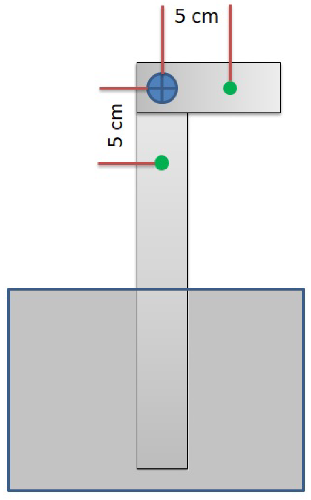
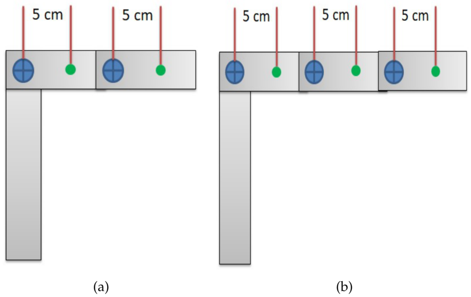
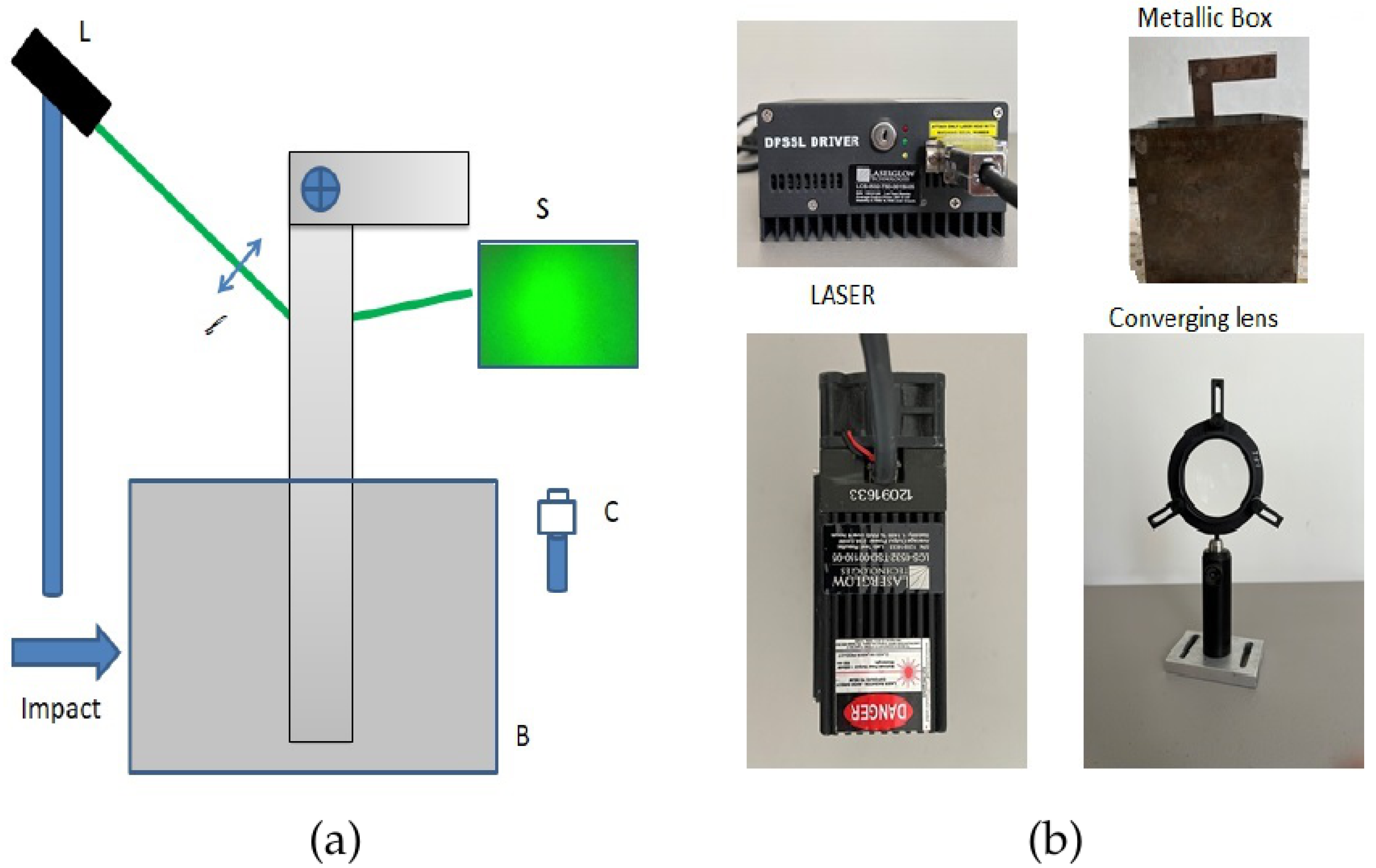
2. Materials and Methods

We used a metallic box built with galvanized sheet caliber 12 (2.695 mm) and dimensions of 40 × 40 × 40 cm, filled with 90% G 0/3 sand, with a density between 1.5 and 1.55 kg/m${}^3$ (Data can be found in Supplementary Materials). This rigid body helped us to fix the metallic arrays, to induce and propagate the impact oscillation. The collisions were performed using a 0.575 kg mass. All impacts were performed exactly on the midpoint of the transversal area at ${30}^{\circ }(\pm 1^{\circ })$. Collisions were performed at room temperature and in light absence. In Figure 1, it is seen the general procedure.

The metallic arrays were made of a smooth steel sheet caliber 16 (1.557 mm). It was cut to make two rectangles: the first of 5 cm width and 40 cm height, and the second of 5 cm width and 20 cm height. Figure 2 shows how optical measurements were made: two impacts were measured 5 cm before the screw and another two 5 cm after. The figure is a cut view of the box and displays the way the array is placed inside the sand. This is how all the arrays are attached to the rigid body.

A similar process is followed for two and three sheet arrays. In the first case Figure 3a, two impacts were measured between both screws, exactly 5 cm after the first, followed by another two 5 cm after the second. Thus, four analyses were performed. For the second case Figure 3b, two collisions were evaluated 5 cm after the first screw, another two 5 cm next to the second, and two more 5 cm next to the third one. Hence, six analyses were performed.

Optical sensing was implemented by using three elements. Firstly, a diode-pumped solid-state laser (L), with a wavelength $\lambda =532$ nm and power of 220 mW [30], was used as the source for the measurements. The second element was a converging lens (ℓ) with a focal length of $f=7$ cm. Finally, the camera (C) recorded slow-motion clips with 1080 p at a 240 fps rate.

In Figure 4, the schematic of the experimental set-up is shown. The laser (L) was placed 40 cm far from the box (B) forming 10${}^{\circ }$ with respect to the perpendicular face of (B). The converging lens (ℓ) was placed in the propagation axis to focus the light beam. The camera (C) was located next to B, avoiding the scattering of the laser and exactly in front of the screen (S). Once the video was recorded, Video-to-JPG-converter was needed because one of its features is to separate the video in each of its possible frames (Information about the software can be found in Supplementary Materials).

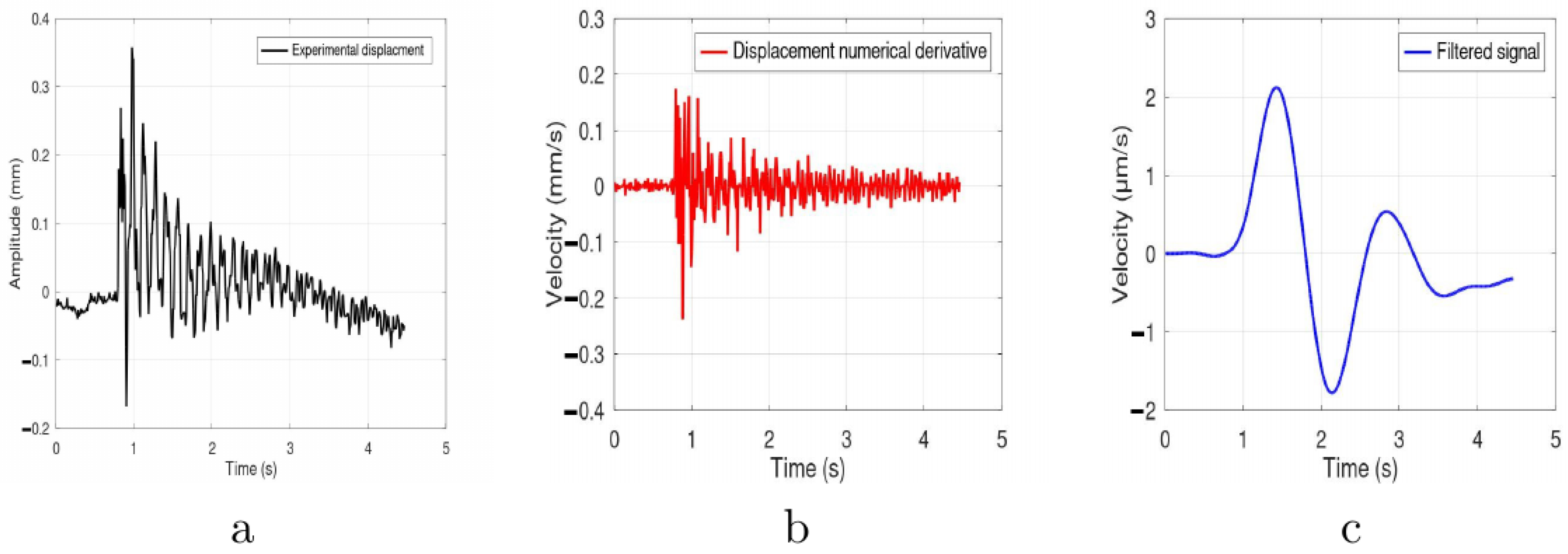
Optical Metrology and Processing

A laser as a source to evaluate the displacements was used. Coherence, unidirectionality, and Gaussian distribution are some of its properties [31]. The last one is relevant since the beam hits a rough material; thus, the reflection can be studied with the probability density function of intensity $P_{\left(I\right)}$:

$$P_{\left(I\right)}=\frac{1}{4\pi {\sigma }^2}ex{p}^{\left(\frac{-I}{2{\sigma }^2}\right)}$$

(1)

where $\sigma$ is the average intensity I of the speckles in the field. The speckles have a very large number of random variables; thus, the central limit theorem is followed [32], as real and imaginary parts of the field are asymptotically Gaussian.

The specklegram is recorded in slow-motion with the camera (C). Then, 2D images are brought out employing free software. Those images are then correlated by code into Octave${}^{\circledR }$, comparing $(A,B)$ in the Fourier domain iteratively, expressing them as the reference and deformed, respectively [3,4,5]. The displacement field can be calculated by:

$$D_f=\frac{Re\left(C_c\right)}{{(s_1\ast s_2)}^{2}M}$$

(2)

where $C_c$ is the mathematical correlation. Normalization is performed, stating M as the image size and $s_1$ and $s_2$ as the standard deviation of the images corresponding to [8,9].

Equation (2) gives a matrix-type result; thus, the maximum amplitude point was logically defined. It is part of the intensity field I in (1), and it is related to the real and imaginary part of the complex amplitude of each speckle [32]. As this is an iterative process, from the second to the n image, those peak amplitudes are plotted as scalar values measured in millimeters according to [8,9].

Before the response was obtained, signal processing by performing a low-pass filter was followed. The obtained result has high-frequency values, and after filtering the signal, the main impact displacement was observed. Also, a numerical first derivative of the signal was proposed. From it, an analytical approach by means of damped and harmonic oscillations was performed. It obtained more than 98% of accuracy by fitting. Finally, an analytical displacement was introduced by means of analytical integrating the function. From this, equivalent movement was observed compared with the experimental results.

3. Results

This section is divided into three parts, beginning with the measurements obtained with a one-sheet array and continuing in consecutive order with two and three steel sheet arrays. The following technique is capable of measuring differences of a few millimeters. In Figure 5a–c, the procedure to study and analyze the results is presented.

Figure 5a is the displacement measurement result by performing a digital image correlation procedure. A post-analysis is followed in Figure 5b. It shows the numerical first derivative obtained through $diff\left(x\right)$. Once performed, high-frequency values were seen; thus, a filtering process was performed implementing a fifth-order $\left(n\right)$ Butterworth low-pass filter by means of $butter(n,\omega c)$. This helped to study the low frequencies, in this case, the impact. A cutoff $\left(\omega c\right)$ and sampling frequency of 240 Hz and 10 kHz were defined, respectively. These values were obtained according to the camera shooter and the oscillation of the solid-state laser used. This filtering analysis is constant along all the presented results. The filtering process was coded into Octave${}^{\circledR }$.

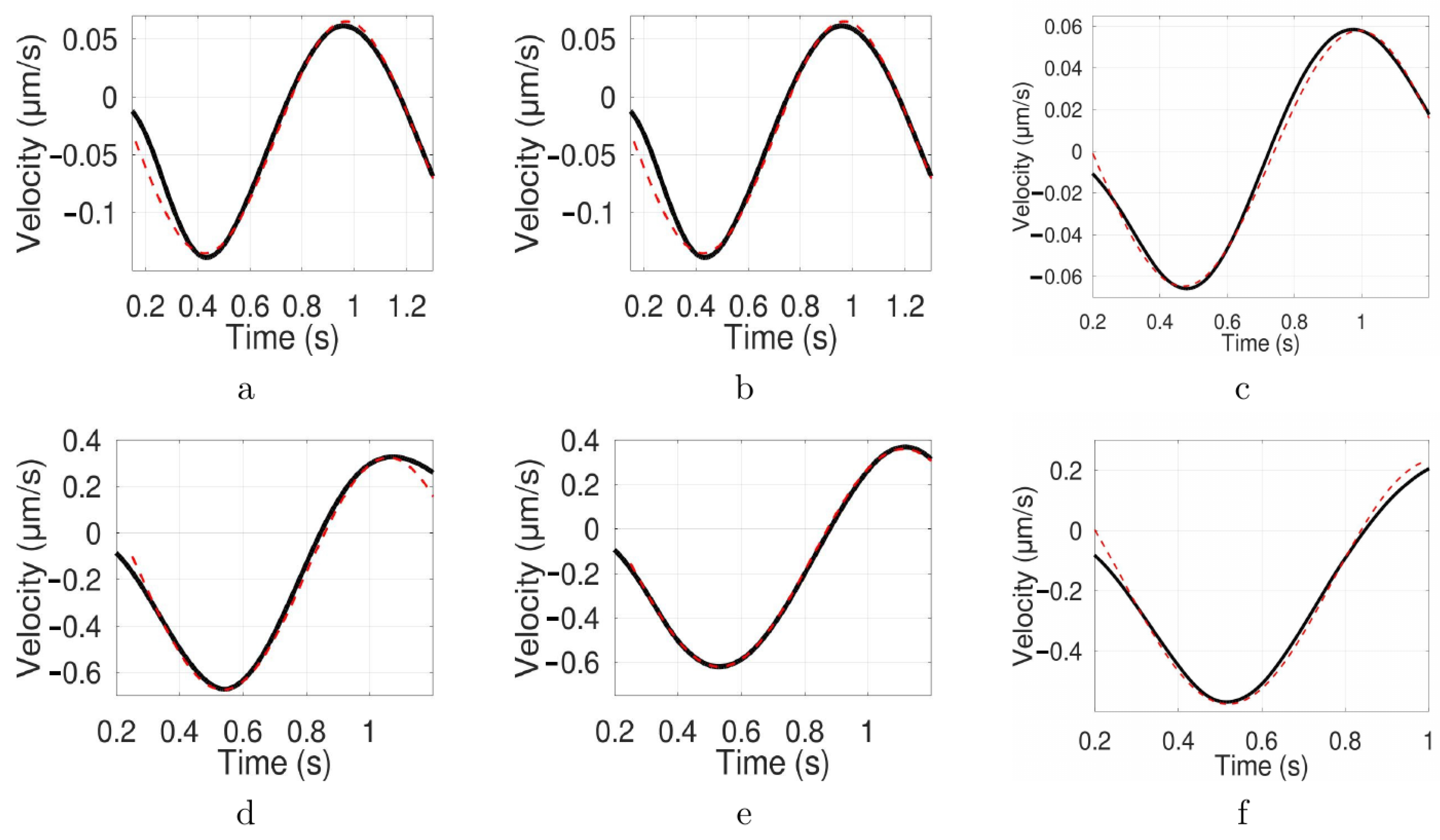
3.1. One-Sheet Array

As aforementioned, the main section is going to be divided into three subsections to show each of the arrays. Recalling Figure 2, these results are focused on measuring 5 cm before and after the screw, as well as the analytical fitting solution. In Figure 6, the graphs for experimental (black) and analytical (red) are displayed.

$$f\left(x\right)=A\ast sin[kx-\omega ]+b$$

(3)

From

Table 1. Values for harmonic solution.

Graph	A (μm)	k (Hz)	$\mathit{\omega }$	b	Relative Error
a	−0.17	5.8	−0.9	−0.035	1.2%
b	−0.17	5.8	−0.9	−0.035	1.2%
c	−0.17	6	+1.9	−0.035	1.4%
d	−0.5	6	−1.65	−0.17	1.1%
e	−0.49	5.4	−1.3	−0.13	0.8%
f	−0.48	5.8	−1.7	−0.17	1.2%

, the analytical solution evidences that the amplitudes were negative, and the frequency had a mean of $5.75$ Hz. Even when (a) had the same values as (b), there were two experimental results that concluded the same analytical solution. The analysis after the screw revealed that the wave amplitude increased.

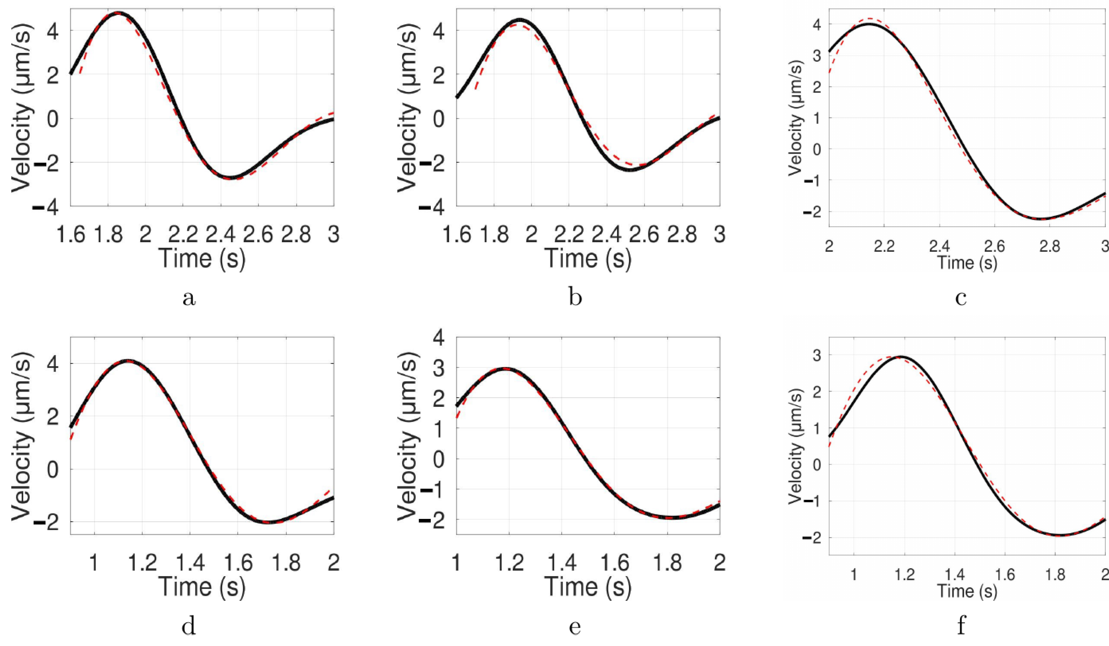
3.2. Two-Sheet Array

Recalling Figure 3a, the order of the measurements is from left to right, beginning after the first screw and then next to the second one. Both analyses were performed 5 cm after the screws.

Figure 7a–d reveals the waveform:

$$f\left(x\right)=A\ast sin[kx-\omega ]\ast exp\left[\beta x\right]-b$$

(4)

Applicable solutions are presented in

Table 2. Resulting values for damped solution.

Graph	A (μm)	k (Hz)	$\mathit{\omega }$	$\mathit{\beta }$	b	Relative Error
a	45	4.9	−1.8	−1.2	−0.1	1.2%
b	46	5	−1.6	−1.4	−0.55	1.3%
c	44	5	−1	−1.8	−0.75	1.5%
d	11	5	−1.45	−1.55	−0.6	1.1%
e	12.6	5.1	−1.25	−1.0	+0.1	1%
f	10.5	4.9	−0.9	−1.0	−0.3	1.2%

, where a mean of 4 $\mathsf{\mu }$m and 5 Hz for amplitude and frequency, respectively, are observed. This waveform had a fitting accuracy greater than $98.5\%$.

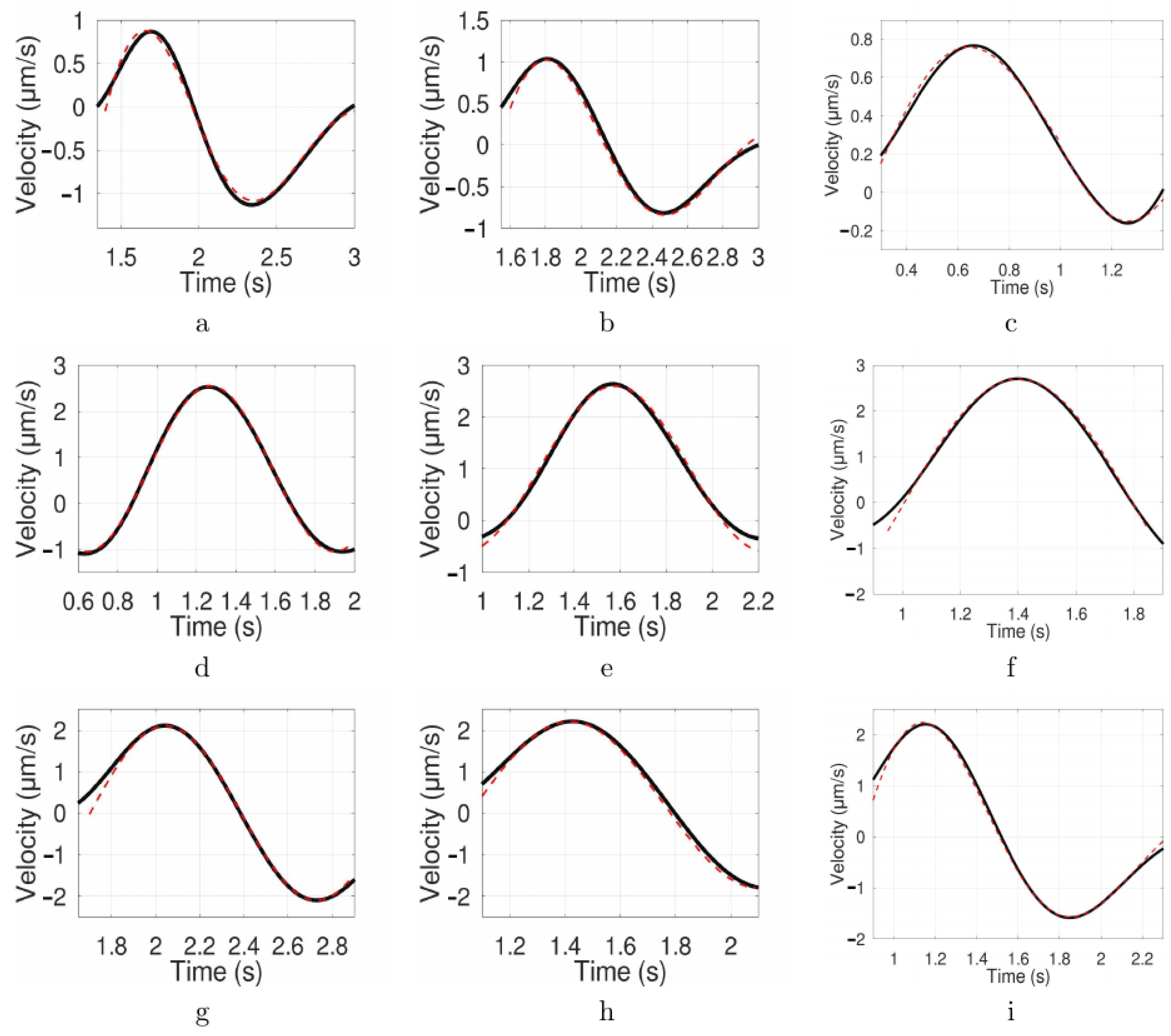
3.3. Three-Sheet Array

The analysis in Figure 3b follows the same order as the latest section, from left to right: after the first screw, next to the second, and next to the third one. All measurements were made 5 cm after each screw.

Figure 8a–i declared both waveforms:

The analytical solutions for this array evidenced both types of oscillations.

Table 3. Values for harmonic and damped solutions.

Graph	A (μm)	k (Hz)	$\mathit{\omega }$	$\mathit{\beta }$	b	Relative Error
a	6.2	4.7	−0.8	−0.9	−0.18	1 %
b	5.8	4.5	+0.2	−0.9	−0.4	1.1 %
c	6	4.6	−1.1	−0.6	+0.4	1 %
Graph	A ($\mathsf{\mu }$m)	k (Hz)	$\omega$	b	Relative Error
d	1.6	4.8	−2.85	1	0.8%
e	1.8	5	+1.5	+0.75	1.2%
f	1.7	5	−0.75	−0.1	1%
g	2	4.6	+1.33	0.2	1.3%
h	2.1	4.6	−1.55	0	1.2%
i	2	4.4	−0.5	0.9	0.8%

is divided into two parts: (a–c) sets the solution for damped oscillations, in which similar amplitude and damping coefficient are observed. The second part (d–i) gives the data that fit the harmonic waveforms. They had related amplitude and frequency values.

3.4. Analytical Discussion

The methodology declared the use of a pendulum oscillation as a way to generate the impacts, where its typical motion equation is:

$$x\left(t\right)=Asin\left[\sqrt{\frac{g}{l}}t\right]$$

(5)

where A, l, and g are the amplitude, the chord length, and the gravity constant, respectively. From Section 3.1, the analytical waveforms obtained in Figure 6 were:

$$f_1\left(x\right)=-0.1\ast sin(5.8x-0.9)-0.035$$

(6)

The values for Equation (4) were taken from Table 1, and performing the integral of it:

$$g_1\left(x\right)=\frac{cos(5.8x-0.9)}{58}-0.035x+c$$

(7)

Figure 9b shows the graph of Equation (7). It displays two parts: first, the incoming oscillation, followed by how it propagates. It can be said that the analytical displacement keeps the waveform of the pendulum, and as a direct consequence, the rigid body and the structural array declare how the wave travels. Also, in Figure 9a, it is seen that the experimental displacement has a similar behavior. The results after the screw were similar since the solution had the same waveform, just different values were obtained. Therefore, analyzing Section 3.2, introducing the values from Table 2, and following the same procedure as before:

$$f_2\left(x\right)=46\ast sin(5x-1.6)\ast exp(-1.4x)-0.55$$

(8)

$$g_2\left(x\right)=\frac{exp(-1.4x)\ast \left[805sin\right(5x-1.6)+2875cos(5x-1.6\left)\right]}{337}-0.55x+c$$

(9)

Figure 9d displays $g_2\left(x\right)$; a peak is present between $0<t<1$ s, which can be associated with the impact reaction. For $t>1$ s, the body, the structure, and the joints decrease the movement. This result is similar to the experimental one. A peak between $0.5<t<1.5$ s can be observed in Figure 9c, followed by a linear decrement.

Section 3.3 shows both waveforms. First, in Figure 8a–c, a damped oscillation as an analytical solution is observed. Then, a harmonic oscillation is present in Figure 8d–i. This result may be associated with the fact that the structure has more weight as well as more rigidity. Inspecting Figure 8, the measurement between screws 1 and 2 is where the damped oscillation occurs; however, between screws 2 and 3 and after the third, the impact propagates as a harmonic oscillation.

According to the analytical solutions shown in [7,8,9], first, the authors declared a sum of two waves as the first analytical approximation to the motion recorded experimentally. This solution gave them an accuracy of 92%. It is important to mention that the waves were a harmonic oscillation plus a damped one, and the experimental data revealed that the movement travels downwards [7]. Years later, the authors announced another analytical approach by solving a damping mass–spring system, in which a damped wave was obtained as a solution. Again, the experimental results evidenced downward movement [8].

Finally, the authors reported another solution for a damped oscillator, in which they showed a combination of harmonic and linear functions [9]. In comparison with these studies, the present article demonstrates that the analytical results reproduced the experimental motion in every array. It adopts harmonic and damped oscillations. The approaches reached more than 98% of accuracy in the impact time-lapse.

On the other hand, filters were used to remove noise frequencies, setting a digital third-order Butterworth low-pass filter with a cutoff frequency of 70 Hz for high-frequency noise [33]. Also, digital filters helped to attenuate the strain spatial resolution in digital image correlation measurements [34]. Additionally, filters were implemented to study gravity measurements [35], handled for medical treatment [36], to remove the noise and detailed texture information [37], to restore images [38], and to study the spatial evolution of phase [39]. All authors improved their results by filtering and setting different cutoff frequencies for each application. Accordingly, the present article proved that by filtering the displacement’s numerical derivative, the impact waveform appears, and it is easier to fit the wave response. Also, it demonstrated that experimental results are equivalent to integrating the analytical approach.

4. Conclusions

This article is about the reaction to an impact in different sets of steel sheets joined by bolts and nuts. The results show that each arrangement propagates the oscillation in a different way. For one sheet, the experimental result revealed that the collision propagates as a harmonic oscillation before and after the screw. For two sheets, the experimental result showed that the shock is transmitted as a damped oscillation in both sections of the steel sheets. The case of three sheets stated a different way of transmission. The first plate showed a damped oscillation, but for the next two sections, the collision propagated harmonically. The modeled waveform for the experimental results demonstrated an accuracy greater than 98%, and the analytical displacement reproduced qualitatively the waveform with respect to the experimental one.

References

1. Proulx, T. Optical Measurements, Modeling, and Metrology, Volume 5, Structural Health Monitoring Using Digital Speckle Photography. In Society for Experimental Mechanics Series; Springer: New York, NY, USA, 2011; Chapter 47; pp. 393–399. [Google Scholar] [CrossRef]
2. Kuglin, C.D.; Hines, D.C. The phase correlation image alignment method. In Proceedings of the International Conference on Cybernetics and Society, Palo Alto, CA, USA, 23–25 September 1975; pp. 163–165. Available online: http://boutigny.free.fr/Astronomie/AstroSources/Kuglin-Hines.pdf (accessed on 3 August 2023).
3. Chevalier, L.; Calloch, S.; Hild, F.; Marco, Y. Digital image correlation used to analyze the multiaxial behavior of rubber-like materials. Eur. J. Mech. A 2010, 20, 169–187. [Google Scholar] [CrossRef] [Green Version]
4. Cintrón, R.; Saouma, V. Strain measurements with digital image correlation system Vic-2D. In Network for Earthquake Engineering Simulation; CU-NEES-08-06; Brown, E.G., Jr., Ed.; Department of Civil Environmental and Architectural Engineering: Boulder, CO, USA, 2008; Available online: https://www.researchgate.net/publication/265230722_Strain_Measurements_with_Digital_Image_Correlation_System_Vic-2D (accessed on 3 August 2023).
5. Pradille, C.; Bellet, M.; Chastel, Y. A Laser speckle method for measuring displacement field. Application to resistance heating tensile test on steel. Appl. Mech. Mater. 2010, 24, 135–140. [Google Scholar] [CrossRef] [Green Version]
6. Barrière, L.; Cherrier, O.; Passieux, J.-C.; Bouquet, M.; Ferrero, J.-F. 3D Digital Image Correlation Applied to Birdstrike Tests; Institute of Research and Technology Saint Exupery: Toulouse, France, 2015. [Google Scholar]
7. Heredia, A.S.; Aguilar, P.A.M.; Villegas, J.A.V. In-plane Displacement Measurement for Analytical Strain Determination. J. Mater. Sci. Eng. 2019, 8, 510. [Google Scholar] [CrossRef]
8. Saldaña-Heredia, A.; Martínez-Calzada, V.; Márquez-Aguilar, P.A.; Hernández-Cruz, D. Optical Characterization of a Pendular Impact. Front. Phys. 2020, 8, 329. [Google Scholar] [CrossRef]
9. Saldaña-Heredia, A.; Martínez-Calzada, V.; Del Villar-Ramírez, V.U.; Rodríguez-Torres, A. Optical measurement of an impact reaction in a modeled wing. Front. Phys. 2022, 10, 770536. [Google Scholar] [CrossRef]
10. Iskander, M. Digital Image Correlation. In Modelling with Transparent Soils; Springer Series in Geomechanics and Geoengineering; Springer: Berlin/Heidelberg, Germany, 2010. [Google Scholar] [CrossRef]
11. Niezrecki, C.; Baqersad, J.; Sabato, A. Digital Image Correlation Techniques for NDE and SHM. In Handbook of Advanced Non-Destructive Evaluation; Ida, N., Meyendorf, N., Eds.; Springer: Cham, Switzerland, 2018. [Google Scholar] [CrossRef]
12. Reddy, K.T.K.; Koniki, S. Digital image correlation for structural health monitoring—A review. E3S Web Conf. 2021, 309, 01176. [Google Scholar] [CrossRef]
13. Mousa, M.A.; Yussof, M.M.; Udi, U.J.; Nazri, F.M.; Kamarudin, M.K.; Parke, G.A.R.; Assi, L.N.; Ghahari, S.A. Application of Digital Image Correlation in Structural Health Monitoring of Bridge Infrastructures: A Review. Infrastructures 2021, 6, 176. [Google Scholar] [CrossRef]
14. Fu, G.; Moosa, A.G. An Optical Approach to Structural Displacement Measurement and Its Application. J. Eng. Mech. 2002, 128, 511–520. [Google Scholar] [CrossRef]
15. Chu, T.P.; Poudel, A. Digital Image Correlation Techniques for Aerospace Applications; Department of Mechanical Engineering and Energy Processes, Southern Illinois University: Carbondale, IL, USA, 2018; p. 62901. [Google Scholar]
16. Kosmann, J.; Völkerink, O.; Schollerer, M.J.; Holzhüter, D.; Hühne, C. Digital image correlation strain measurement of thick adherend shear test specimen joined with an epoxy film adhesive. Int. J. Adhes. Adhes. 2019, 90, 32–37. [Google Scholar] [CrossRef]
17. Johansson, M.; Rempling, R.; Sanz, G.; Zanuy, C. Key aspects of digital image correlation in impact tests of reinforced concrete beams. In Proceedings of the Guimaraes 2019: Towards a Resilient Built Environment Risk and Asset Management, Guimarães, Portugal, 27–29 March 2019. Report: 961-968. [Google Scholar]
18. Chai, J.; Liu, Y.; Yang, B.Y.; Zhang, D.; Du, W. Application of Digital Image Correlation Technique for the Damage Characteristic of Rock-like Specimens under Uniaxial Compression. Adv. Civ. Eng. 2020, 2020, 8857495. [Google Scholar] [CrossRef]
19. Winkler, J.; Duus Hansen, M. Innovative Long-Term Monitoring of the Great Belt Bridge Expansion Joint Using Digital Image Correlation. Struct. Eng. Int. 2018, 28, 347–352. [Google Scholar] [CrossRef]
20. Ledford, N.; Paul, H.; Isakov, M.; Hiermaier, S. High rate loading of hybrid joints in a Split Hopkinson Tension Bar. EPJ Web Conf. 2018, 183, 2023. [Google Scholar] [CrossRef] [Green Version]
21. Souto Janeiro, A.; Fernández López, A.; Chimeno Manguan, M.; Pérez Merino, P. Three Dimensional Digital Image Correlation Based on Speckle Pattern Projection for Non Invasive Vibrational Analysis. Sensors 2022, 22, 9766. [Google Scholar] [CrossRef]
22. Timbolmas, C.; Rescalvo, F.J.; Portela, M.; Bravo, R. Analysis of poplar timber finger joints by means of Digital Image Correlation (DIC) and finite element simulation subjected to tension loading. Eur. J. Wood Prod. 2022, 80, 555–567. [Google Scholar] [CrossRef]
23. Chaves, C.E.; Fernandez, F.F. A review on aircraft joints design. Aircr. Eng. Aerosp. Technol. 2016, 88, 411–419. [Google Scholar] [CrossRef]
24. Bunin, B.L. Critical Joints in Large Composite Primary Aircraft Structures: Volume I—Technical Summary (NASA Contractor Report 3914); Prepared for Langley Research Center under Contract NAS1-16857; Douglas Aircraft Company: Long Beach, CA, USA, 1986. [Google Scholar]
25. Li, H.; Li, X.; Yang, Y.; Liu, Y.; Ma, M. Structural Stress Characteristics and Joint Deformation of Shield Tunnels Crossing Active Faults. Appl. Sci. 2022, 12, 3229. [Google Scholar] [CrossRef]
26. Hristovska, E.; Stavreva, S. Stress and Deformation Analysis of Joint Plate Depending on Truss Joint Design of Carrying Structure. TEM J. 2021, 10, 892–899. [Google Scholar] [CrossRef]
27. Ivan, H.; Iyad, A. Connections and Joints in Precast Concrete Structures. Slovak J. Civ. Eng. 2020, 28, 49–56. [Google Scholar] [CrossRef]
28. Santos, M.A.S.; Campilho, R.D.S.G. Experimental and numerical analysis of the fracture envelope of composite adhesive joints. Sci. Technol. Mater. 2018, 30, 131–137. [Google Scholar] [CrossRef]
29. Kendall, O.; Paradowska, A.; Abrahams, R.; Reid, M.; Qiu, C.; Mutton, P.; Yan, W. Residual Stress Measurement Techniques for Metal Joints, Metallic Coatings and Components in the Railway Industry: A Review. Materials 2023, 16, 232. [Google Scholar] [CrossRef]
30. Laserglow Technologies. LCS-0532 Low-Cost DPSS Laser System; Laserglow Part Number: C53200XSX, Laser Product Datasheet Generated on 2015; Laserglow Technologies: North York, ON, Canada, 2015. [Google Scholar]
31. BahaaSaleh, E.A.; Teich, M.C. Fundamentals of Photonics; John Wiley and Sons: Hoboken, NJ, USA, 1991. [Google Scholar]
32. Dainty, J.C. Laser Speckle and Related Phenomena; Springer: Berlin/Heidelberg, Germany; New York, NY, USA, 1975. [Google Scholar]
33. Qian, J.; Tiwari, P.; Gochhayat, S.P.; Pandey, H.M. A Noble Double-Dictionary-Based ECG Compression Technique for IoTH. IEEE Internet Things J. 2020, 7, 10160–10170. [Google Scholar] [CrossRef]
34. Reu, P.L.; Blaysat, B.; Andó, E.; Bhattacharya, K.; Couture, C.; Couty, V.; Deb, D.; Fayad, S.S.; Iadicola, M.A.; Jaminion, S.; et al. DIC Challenge 2.0: Developing Images and Guidelines for Evaluating Accuracy and Resolution of 2D Analyses. Exp. Mech. 2022, 62, 639–654. [Google Scholar] [CrossRef]
35. Bidel, Y.; Zahzam, N.; Bresson, A.; Blanchard, C.; Cadoret, M.; Olesen, A.V. Absolute airborne gravimetry with a cold atom sensor. J. Geod. 2020, 94, 20. [Google Scholar] [CrossRef] [Green Version]
36. Chu, M.; Nguyen, T.; Pandey, V.; Zhou, Y.; Pham, H.N.; Bar-Yoseph, R.; Radom-Aizik, S.; Jain, R.; Cooper, D.M. Respiration rate and volume measurements using wearable strain sensors. NPJ Digit. Med. 2019, 2, 8. [Google Scholar] [CrossRef] [PubMed] [Green Version]
37. Lee, B.; Oh, J.Y.; Cho, H.; Joo, C.W.; Yoon, H.; Jeong, S.; Oh, E.; Byun, J.; Kim, H.; Lee, S.; et al. Ultraflexible and transparent electroluminescent skin for real-time and super-resolution imaging of pressure distribution. Nat. Commun. 2020, 11, 663. [Google Scholar] [CrossRef] [Green Version]
38. Amer, K.O.; Elbouz, M.; Alfalou, A.; Brosseau, C.; Hajjami, J. Enhancing underwater optical imaging by using a low-pass polarization filter. Opt. Express 2019, 27, 621–643. [Google Scholar] [CrossRef]
39. Kulkarni, R.; Rastogi, P. Simultaneous unwrapping and low pass filtering of continuous phase maps based on autoregressive phase model and wrapped Kalman filtering. Opt. Lasers Eng. 2020, 124, 105826. [Google Scholar]
Figure 1. Experimental set-up of the impact induction: (a) 2D image illustration; (b) real picture.
Applsci 13 09275 g001
Figure 2. Optical measurement in a one-sheet array.
Applsci 13 09275 g002
Figure 3. Metrology system in arrays: (a) two and (b) three steel sheets.
Applsci 13 09275 g003
Figure 4. Experimental set-up: (a) 2D illustration; (b) used devices.
Applsci 13 09275 g004
Figure 5. Signal processing: (a) experimental displacement; (b) numerical first derivative; (c) filtered signal.
Applsci 13 09275 g005
Figure 6. One-sheet array graphs: (ac) analysis before the screw; (df) solution after the screw.
Applsci 13 09275 g006
Figure 7. Two-sheet array graphs: (ac) analytical solution after the first screw; (df) next to the second one.
Applsci 13 09275 g007
Figure 8. Graphs according to measurements along a three-sheet array: (ac) after the first screw; (df) next to the second screw; (gi) next to the third one.
Applsci 13 09275 g008
Figure 9. Displacement comparative: (a) experimental harmonic oscillation; (b) analytical g 1 ( x ) ; (c) experimental damped oscillation; (d) analytical g 2 ( x ) .
Applsci 13 09275 g009