Abstract
When dealing with specific tasks, the hidden layer output matrix of an extreme learning machine (ELM) may change, largely due to the random assigned weight matrix of the input layer and the threshold matrix of the hidden layer, which sequentially leads to the corresponding change to output weights. The unstable fluctuations of the output weights increase the structural risk and the empirical risk of ELM. This paper proposed a fuzzy adaptive particle swarm optimization (PSO) algorithm to solve this problem, which could nonlinearly control the inertia factor during the iteration by fuzzy control. Based on the fuzzy adaptive PSO-ELM algorithm, a sound quality prediction model was developed. The prediction results of this model were compared with the other three sound quality prediction models. The results showed that the fuzzy adaptive PSO-ELM model was more precise. In addition, in comparison with two other adaptive inertia factor algorithms, the fuzzy adaptive PSO-ELM model was the fastest model to reach goal accuracy.
1. Introduction
With the development of the automobile industry, people have more stringent requirements for the acoustic characteristics of vehicles, not only limited to traditional acoustic indicators such as sound pressure but also including acoustic annoyance [1,2,3]. The issue of in-car sound quality has also received more attention from designers.
Sound quality reflects the listener’s acceptance of the sound; the higher the acceptance level, the better the sound quality. The evaluation of sound quality includes two parts: objective evaluation and subjective evaluation of sound samples. The loudness, sharpness, and clarity of sound all have an impact on sound comfort, so scholars have put forward many objective evaluation parameters of sound quality by considering acoustic physical parameters such as sound pressure, frequency, and other characteristics of human auditory perception such as characteristic frequency band and auditory masking effect [4,5]. Common objective evaluation parameters of sound quality include loudness, roughness, sharpness, etc. There are many subjective evaluation methods for sound quality, among which the rating scale method [6], semantic segmentation method [7,8], and comparison method [9] are more mature. Each method applies to different scenarios and the number of sound samples, evaluation targets, and other factors need to be considered when designing measurement tests. The above methods may be influenced by the evaluator’s subjective emotions, perceptions, or evaluation environment, which can easily lead to bias between the results and true feelings. Therefore, Li [10] proposed that the sound quality could be evaluated by electroencephalograph (EEG).
The basic process of sound quality evaluation includes sound sample collection, sound quality evaluation grouping, objective sound quality evaluation, subjective sound quality evaluation, and statistical multiple regression. By analyzing the correlation between subjective parameters and objective parameters, finally a sound quality evaluation model is established [11,12]. Among them, how to establish the relationship between the subjective parameters and objective parameters of sound quality has become a key issue that researchers are concerned about.
Many scholars use different neural network methods to predict sound quality, including back propagation neural network (BPNN) [13,14], deep convolutional neural networks (CNNs) [15], radial basis function (RBF) [16], genetic algorithm [17], and others [18,19,20,21]. Hou [6] built the standard BPNN model, the genetic algorithm back propagation neural network (GA-BPNN) model and back propagation neural network based on particle swarm optimization (PSO) and proved that the PSO-BPNN model can achieve convergence more quickly and improve the prediction accuracy of sound quality. Mehdi [22] developed an improved intelligent model that combines the optimal analytic wavelet transform (OAWT) and the PSO-BPNN model. The new model has higher accuracy and much lower computational load. Zhang [23] established two sound quality evaluation models based on the BPNN algorithm and the support vector machine (SVM) algorithm. The accuracy of the SVM model is better than the BPNN model when the sample size is insufficient. Huang [24] proposed regression-based deep belief networks (DBNs) to predict the sound quality, which substitute the support vector regression (SVR) layer for the linear soft max classification layer at the top of the general DBN’s structure. The accuracy and robustness of the proposed DBN-based sound quality prediction model have been significantly improved.
The extreme learning machine (ELM) is a single hidden layer feedforward neural network algorithm with high learning efficiency and good generalization performance [25]. In recent years, it has been applied to more and more fields [26,27,28,29,30]. Compared with common neural networks, RBF neural networks, wavelet neural networks, convolutional neural networks, support vector machines, and deep learning methods, ELM methods have some advantages in the following three aspects:
- (1)
- Short learning time. ELM does not need to set the network weights; the hidden layer weights and threshold values are obtained in a random way, so the learning rate is very fast.
- (2)
- Simple algorithm implementation. It can be computed quickly by simply setting the network structure parameters.
- (3)
- Strong generalization ability. The general neural network training process is prone to the phenomenon of “overfitting”, but ELM has a strong generalization ability.
Therefore, this paper selects the ELM to establish the sound quality prediction model. The input is objective parameter and the output is subjective parameters of sound quality.
However, the weight matrix and the threshold matrix of the ELM neural network are randomly generated, resulting in a non-full rank of the hidden layer output matrix and reducing the prediction accuracy of the ELM model [31]. Particle swarm optimization (PSO) is a numerical optimization algorithm inspired by the foraging behavior of birds that can adjust the connection weights and thresholds. PSO algorithm is based on “information sharing”. It has the advantages of fast convergence, few parameters, and simple algorithm implementation. Consequently, in this paper, the fuzzy adaptive particle swarm optimization (PSO) algorithm is used to optimize the selection of the weight matrix and the threshold of ELM.
2. Fuzzy Adaptive PSO-ELM Prediction Model
2.1. Extreme Learning Machine
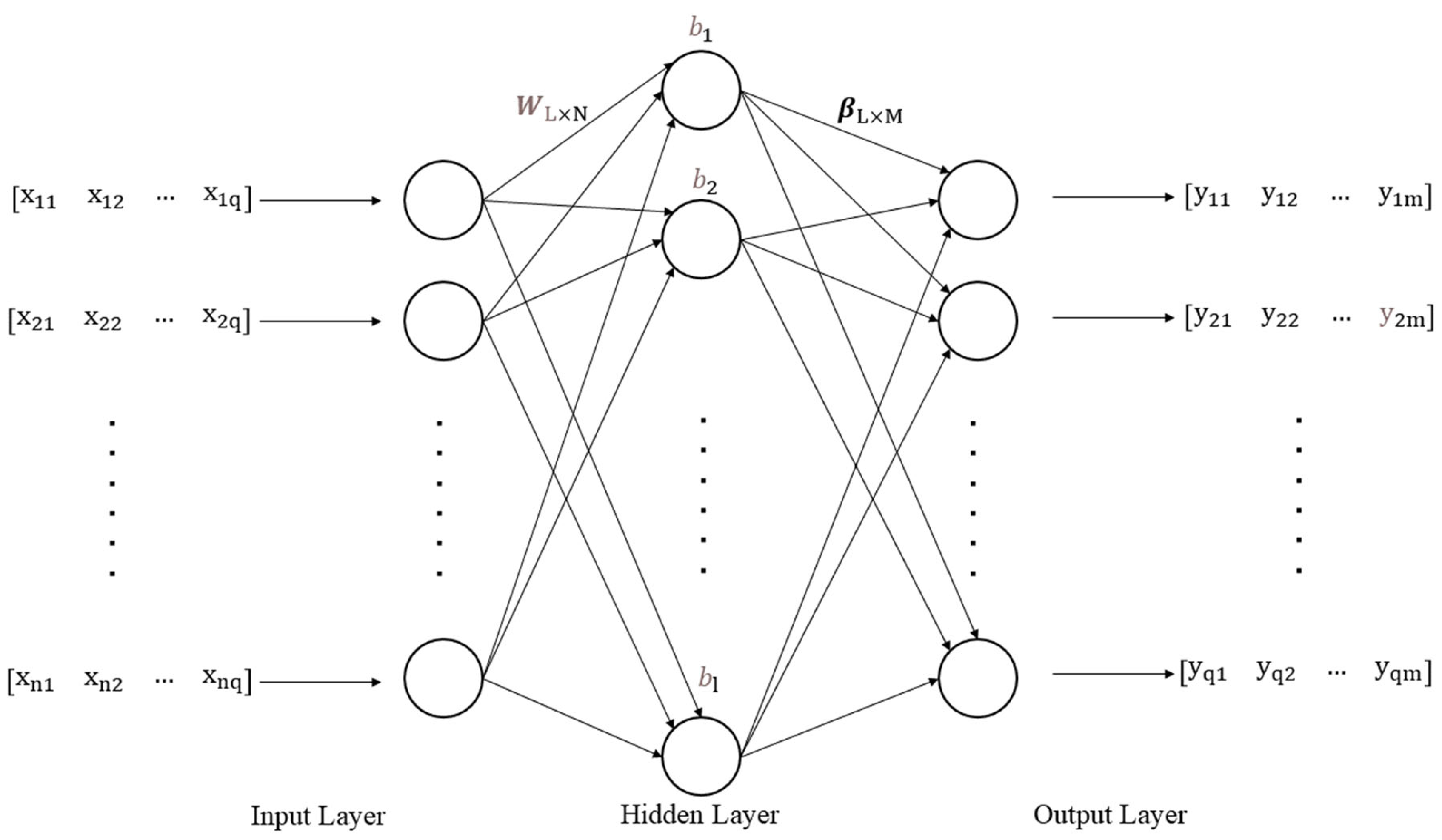
The extreme learning machine (ELM) (Figure 1) neural network structure is as follows:
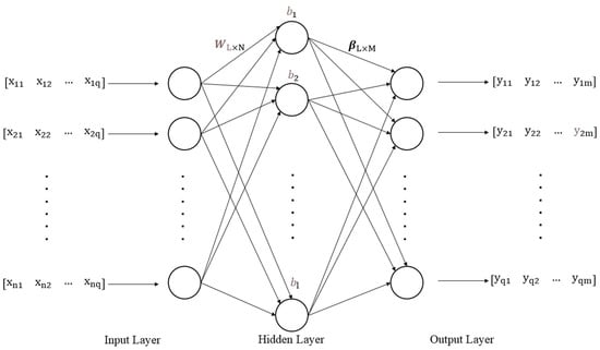
Figure 1.
Extreme learning machine (ELM) neural network structure.
The ELM neural network structure consists of three parts, from left to right, the input layer, the hidden layer, and the output layer. Each layer is connected to each other by a feature weight matrix and the information from the input layer is processed by the hidden layer and passed to the output layer, which feeds us the desired result according to the feature weight matrix.
The ELM neural network structure where is the number of neurons in the input layer; is the number of the sample; is the number of neurons in the hidden layer; is the number of neurons in the output layer; is the input matrix; is the weight matrix connecting the input layer and the hidden layer; is the threshold matrix of the hidden layer; is the weight matrix connecting the hidden layer and the output layer; is the theoretical output matrix:
The ELM algorithm can randomly generate the weight matrix connecting the input layer and the hidden layer, as well as the threshold matrix of the hidden layer, which do not change.
The output of hidden layer is
In the formula: is the activation function, which is Sigmoid function
The theoretical output matrix of ELM is
The weight matrix is solved by minimizing the approximate norm squared difference between the theoretical output and the actual output
It is assumed that the algorithm provides an error-free approximation.
According to Moore–Penrose (MP) generalized inverse matrix theory and Karush–Kuhn–Tucker (KKT) conditions, the hidden layer weight is
In the formula, is the penalty coefficient and finally the output function expression of the ELM algorithm is obtained
2.2. Fuzzy Adaptive Particle Swarm Optimization
In this paper, the particle swarm optimization (PSO) algorithm is used to optimize the weight matrix and the threshold of ELM, which has the advantages of fast convergence, high learning efficiency, and high accuracy.
Particle swarm optimization is a swarm intelligence optimization algorithm. The PSO can find the optimal solution by collaboration and information sharing among individuals in the group.
The PSO algorithm initializes the maximum number of iterations and population size at first. Then, it determines the spatial dimension of particle search D.
In the PSO algorithm for optimizing the weights and thresholds of ELM, each particle in the solution space contains all the weights and thresholds of a network.
The initial position and velocity of each particle are randomly defined. After each iteration, the fitness function evaluates the state of each particle and selects the group optimal value and the individual optimal value in the population. The position and velocity of each particle are updated through both of them. If the solution of the current particle is better than the previously recorded individual optimal value or the group optimal value , then it is the new optimal solution.
The position and velocity of each particle are updated by Formulas (15)–(17)
where is the number of iterations; is the inertia factor, which has a great influence on the performance of the PSO. The larger w is the more active the particle is in exploring new regions in the search space, which shows better global search ability; the smaller w is the more the particle is influenced by the current environment, which shows better local search ability; is the velocity of the particle at iterations; is the position of the particle at iterations; is individual optimal value at iterations; is group optimal value at iterations; and are the learning factors, where reflects how well the particle trusts its own experience; reflects how well the particle trusts the information passed on by other particles; and are random numbers between 0 and 1; and are the velocity boundaries; and are the particle position boundaries.
By defining the fitness function, , the PSO algorithm iteratively obtains the optimal population. This is used as the weight and threshold of the ELM to obtain the predicted output after training.
Due to the influence of the inertia factor , the convergence speed of PSO is not quick and stable. Many researchers use a linear decreasing method to control . However, its changes are unknown; in other words, iteration may not linearly change.
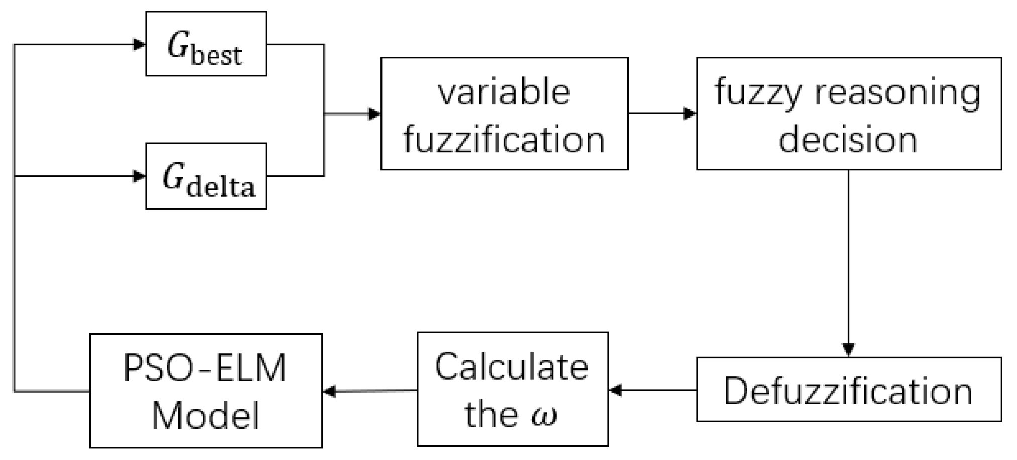
This paper used a fuzzy controller to change adaptively, which has better nonlinear control ability. The fuzzy controller utilizes the principles of fuzzy mathematics to realize nonlinear control well, including the following five parts: defining variables, fuzzification, establishing rule tables, logical reasoning, and output defuzzification. The and its decreasing rate in the PSO are treated as input variables and the adaptive is the output of the fuzzy controller. Figure 2 shows the process of the fuzzy controller.

Figure 2.
The process of model building.
The variables are all fuzzified into three fuzzy subsets: positively big PB, positively middle PM, and positively small PS and the shape of membership function is defined as triangle.
3. Subjective and Objective Evaluation Models of Sound Quality
3.1. Objective Evaluation Parameters of Sound Quality
The loudness, sharpness, and clarity of sound all have an impact on sound comfort. To provide a comprehensive description of sound quality, this paper analyzes the A-weighting sound pressure level, loudness, roughness, fluctuation, and sharpness.
Due to the wide range of hearing thresholds of the human ear, sound strength cannot be described directly using sound pressure. As a result, it is converted to sound pressure level by taking its logarithm, which is expressed as follows:
where is the sound pressure and is the reference sound pressure.
The A-weighting sound pressure level considers the impact of sound frequency on human hearing sensitivity. It can be adjusted according to different frequency bands to better reflect the human ear’s true perception of sound intensity.
The loudness of a sound corresponds to its strength. The calculations based on the Zwicker loudness theory consider the auditory masking effect and the eigenfrequency bands.
The variable represents the sound pressure level at the central frequency in the current condition. The variable represents the sound pressure level at the central frequency in the hearing threshold under quiet conditions (meaning the sound pressure level corresponding to each critical central frequency on the isophonic curve).
Roughness and fluctuation are both used to describe how the human ear perceives changes in the time domain of sound. According to Zwicker’s theory, roughness and fluctuation are modeled as follows:
where is the modulation depth and is the modulation frequency.
Sharpness is used to describe the pitch of a sound. The greater the sharpness, the higher the pitch of the sound.
where C is the coefficient and is the number of characteristic frequency bands.
3.2. Subjective Evaluation Test of Sound Quality
A specific brand of passenger car was selected as the research subject. The experiment took place on a flat asphalt road with a smooth surface and no unnecessary obstacles nearby. The vehicular noise signals were recorded using LMS Test.Lab, with microphones placed at the primary driver’s right ear and at the center of the rear seat of the car. The operational conditions included maintaining constant speeds of 20 km/h, 40 km/h, and 50 km/h, as well as performing full-throttle acceleration from 0 to 70 km/h. Every operational scenario was recorded multiple times, with each sound sample lasting for at least 40 s. A segment was made from each of the 60 recorded sample sets to erase any abnormal noises during the test procedure caused by human factors. From this, a selected dataset of 30 sound samples was obtained. Then, the effective sound segments were reduced to 5 s, leading to a final dataset of 30 sound samples.
In this paper, the subjective feeling of comfort is used to score the samples on different levels. According to the international standard, the comfort level is divided into 11 levels; the comfort scoring criteria shown in Table 1 are established.

Table 1.
Results of the subjective and objective evaluation.
A total of 20 participants, consisting of 13 males and 7 females, participated in the assessment of sound quality. As a result of the lengthy test, the evaluator was likely to experience fatigue and irritation, which could result in misjudgments. We included five pairs of identical samples in the test as a means of calculating the accuracy of subjective evaluations. An evaluator’s evaluation was accurate when samples A and B were equal; otherwise, it was a misjudgment. After evaluating the testers’ accuracy rates, we adjusted the test data by excluding three sets with lower accuracy rates. The arithmetic mean of the subjective ratings corresponding to each noise sample was calculated.
4. Application of Sound Quality Prediction Model
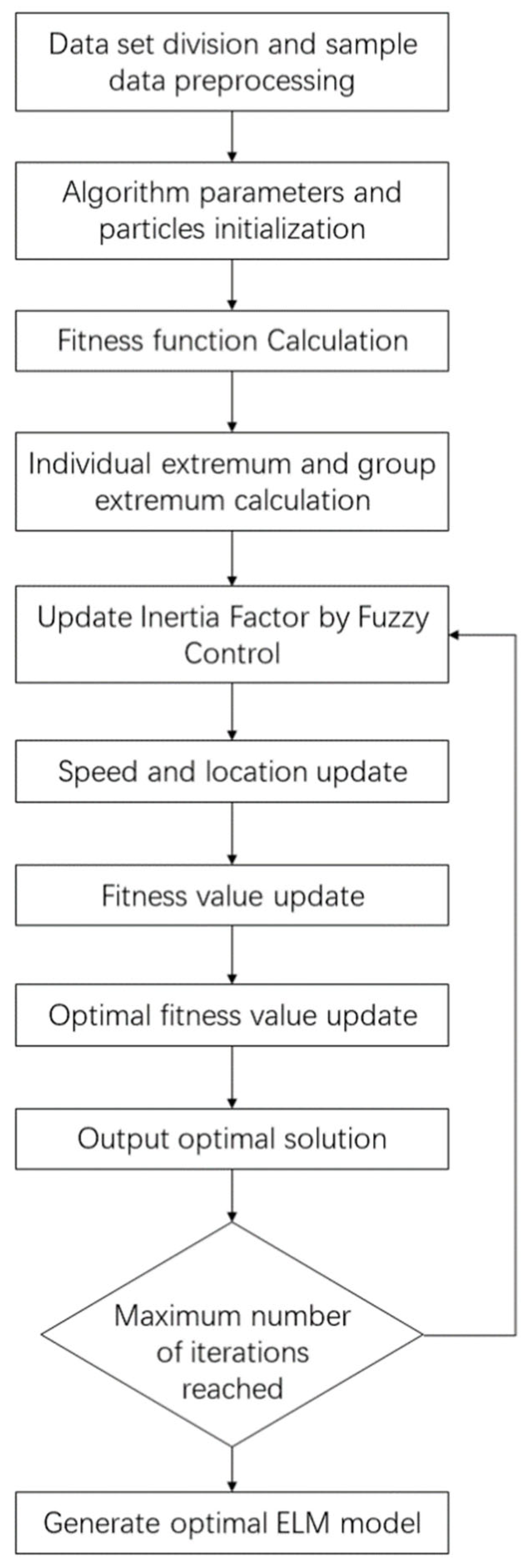
Sound quality is a multiparameter comprehensive evaluation method which is completely different from traditional acoustic evaluation indicators. It includes objective and subjective assessments of sound samples. Establishing the relationship between subjective and objective parameters of sound quality is particularly significant. The outcomes of this approach align more closely with the human ear’s subjective perception, as it eliminates the laborious procedure of subjective assessment tests and the unpredictability of human variables. The ELM neural network is optimized using the fuzzy adaptive PSO algorithm, which offers the advantages of fast convergence, high learning efficiency, and high accuracy. Objective parameters of sound quality are used as input matrix and the subjective parameters of sound quality is treated as the output matrix. Figure 3 shows the establishment process of the fuzzy adaptive PSO-ELM sound quality prediction model.

Figure 3.
The process of model building.
- First step:
Five representative sound quality objective parameters, including A-weighting sound pressure level, loudness, roughness, fluctuation, and sharpness, were used to predict the comfort of the sound quality subjective parameters.
The first step was normalizing the five objective parameters of sound quality. Then, the numbered samples were randomized and split into training and test sets.
In order to compare the prediction results and verify the superiority of the algorithm, the first 25 groups listed in Table 2 served as the training set, while the last 5 groups acted as the test set.
Table 2.
Results of the subjective and objective evaluation.
- Second step:
The elements of and randomly generated in ELM were normalized and reorganized into one matrix as PSO particles. groups particles formed a population. Then, parameters were set, as shown in Table 3.
Table 3.
Parameter settings.
- Third step:
The fitness function is defined as
In the first iteration, the particle fitness value of the whole population was calculated and substituted and the optimal particle fitness value was obtained. Because of the first iteration, optimal population fitness value and the optimal particle position was the particle, whose fitness value was .
- Fourth step:
The inertia factor, , was updated according to the fuzzy control rules. In order to make the fitness function converge rapidly with iterating and not easily fall into local minimum value, the rules were as Table 4, which were determined by experience. When the population optimal fitness value was larger and the change of the population optimal fitness value was larger, the inertia factor was larger. When the population optimal fitness value was smaller and the change of the population optimal fitness value was smaller, the inertia factor was smaller.
Table 4.
Fuzzy Control Rules.
The population according to Formulas (15)–(17) was updated, new ELM networks were generated, and the population was re-substituted to obtain the new optimal fitness value and position. If was smaller than , and would be replaced by and the particle whose fitness value was .
- Fifth step:
When the maximum number of iterations was reached, the optimal fitness value and position were output and could be expanded to the optimal weight matrix and threshold matrix .
- Sixth step:
Using the input layer weight matrix and the hidden layer threshold matrix , which was obtained by the fuzzy adaptive PSO algorithm, an optimal ELM neural network model was constructed to predict the annoyance.
5. Prediction Result
The weight matrix and the threshold matrix of the fuzzy adaptive PSO-ELM model of the sound quality prediction after training is shown in Table 5. The parameters were put into Formulas (6), (12) and (13). The subjective annoyance of sound quality could be obtained by calculating objective evaluation parameters and substituting them into the established mathematical model.
Table 5.
Matrixes of weights and thresholds.
The prediction results’ evaluation used [6] and the goodness of fit
In the formula, represented prediction value, which was equivalent to in this article; represented experiment value, which was equivalent to in this article; represented relative error.
Figure 4 shows prediction results of the fuzzy adaptive PSO-ELM model.
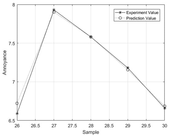
Figure 4.
Prediction results of test set.
Table 6 presents three other different prediction models in the literature [6]. The results show that the relative error of the fuzzy adaptive PSO-ELM model was 0.73% and the goodness of fit was 0.981, which was much better than the other three models (the BP model was 4.45%, the GA-BP model was 3.31%, and the PSO-BP model was 1.64%).
Table 6.
Prediction results of four different models.
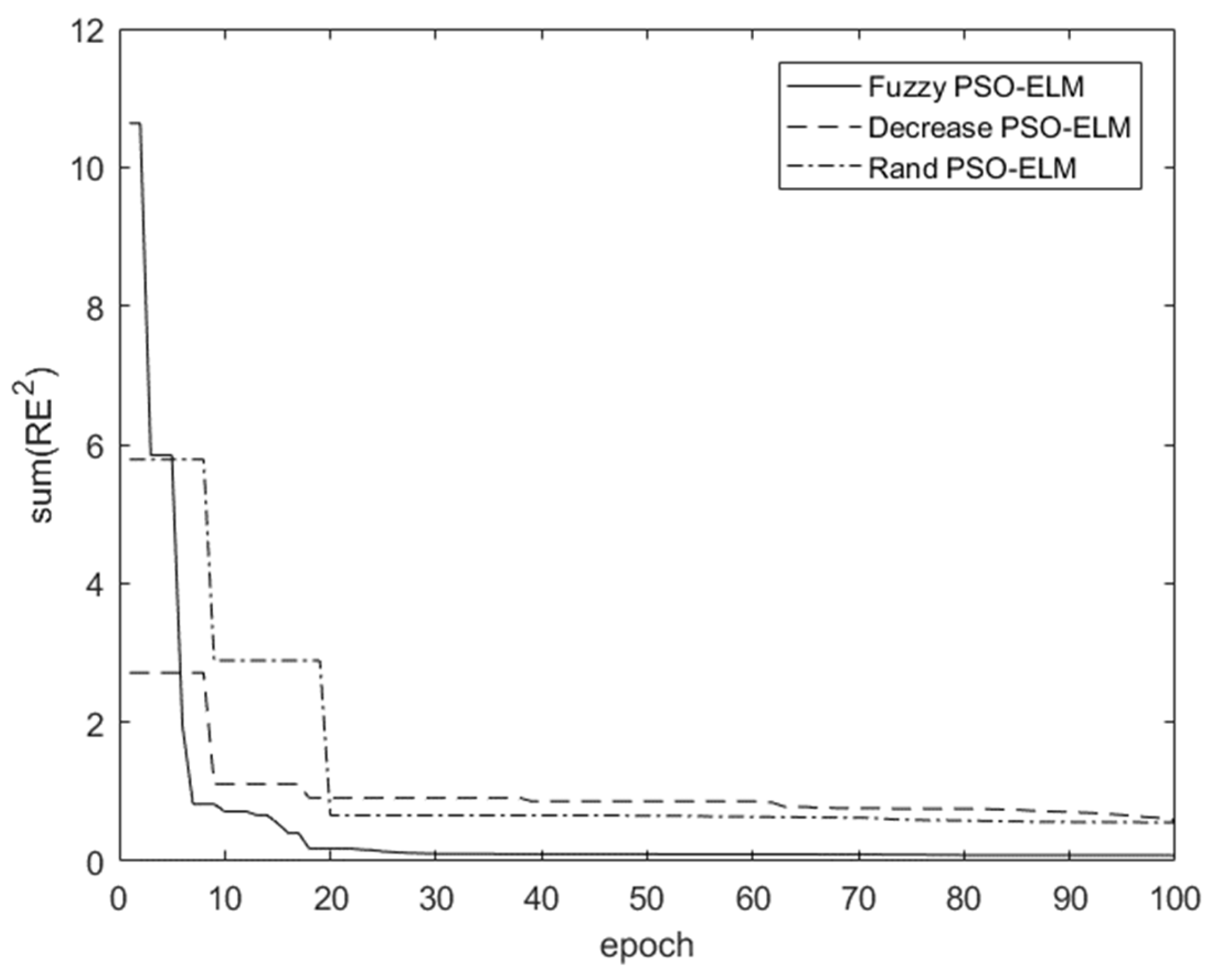
Three different adaptive inertia factor control methods —fuzzy adaptive PSO-ELM model, rand (ω) PSO-ELM model, and decreasing (ω) PSO-ELM model—were selected and compared:
Figure 5 shows that the rand (ω) PSO-ELM model tended to be flat at the 20 epochs, with a slight drop at the 70 epochs, which meant the rand (ω) PSO-ELM model easily fell into the local minimum. The convergence process of the decreasing (ω) PSO-ELM method was long; the optimal solution had obviously not been found. The fuzzy adaptive PSO-ELM model could rapidly converge within 30 epochs and was more accurate than the other methods. Therefore, in order to achieve the same prediction accuracy, the fuzzy adaptive PSO-ELM model was fastest. And the fuzzy adaptive PSO-ELM model could achieve higher precision when the iteration time was the same and it was not easily trapped in the local minimum.

Figure 5.
Three adaptive inertia factor control models.
6. Conclusions
The weight matrix of the input layer and the threshold matrix of the hidden layer were randomly generated at the beginning of the ELM, which led to the low prediction accuracy. To solve this problem, this paper proposed the fuzzy adaptive PSO-ELM model, which could achieve higher precision rapidly. Fuzzy control was used to realize the nonlinear control of the inertia factor of PSO. Seven kinds of objective parameters of sound quality were used as input and the annoyance was used as output. The result showed the following factors.
Comparing the prediction results of the fuzzy adaptive PSO-ELM model, the BPNN model, the GA-BPNN model, and the PSO-BPNN model, the fuzzy adaptive PSO-ELM model had the best prediction precision, with an average error of 0.73% and a goodness of fit of 0.981.
Comparing the iterative processes of the fuzzy adaptive PSO-ELM model, rand (ω) PSO-ELM model, and decreasing (ω) PSO-ELM model, the fuzzy adaptive PSO-ELM model needed the least number of iterations when achieving the same prediction accuracy. The rand (ω) PSO-ELM model fell easily into local minimum. The convergence process of the decreasing (ω) PSO-ELM method was long. The fuzzy adaptive PSO-ELM model could achieve higher accuracy and higher algorithm efficiency at the same epoch.
The fuzzy adaptive PSO-ELM model connected the objective and subjective sound quality evaluation parameters. It accurately predicted subjective sound quality evaluations based on objective parameters, which reduced testing expenses and time. This model provided a dependable way of predicting automobile sound quality with practical implications.
Author Contributions
Writing—review and editing, C.W.; writing—original draft, G.Y.; project administration, J.L. and Q.H. All authors have read and agreed to the published version of the manuscript.
Funding
This research was funded by Guangxi Science and Technology Major Program (grant number GuikeAA22068060-6) and Valeo—HUST Joint Vibration and Acoustic Laboratory.
Institutional Review Board Statement
Not applicable.
Informed Consent Statement
Not applicable.
Data Availability Statement
The data used to support the findings of this study are included within the article.
Conflicts of Interest
The authors declare no conflict of interest.
References
- Geng, Y.T.; Nakayama, M.; Nishiura, T. Demodulated sound quality improvement for harmonic sounds in over-boosted parametric array loudspeaker. Appl. Acoust. 2022, 186, 108460. [Google Scholar] [CrossRef]
- Wang, X.L.; Song, Y.C.; Liu, N.N. Hybrid vibro-acoustic active control method for vehicle interior sound quality under high-speed. Appl. Acoust. 2022, 186, 108419. [Google Scholar] [CrossRef]
- Liu, Z.E.; Li, X.L.; Zheng, Q.Q. Strategy and implementing techniques for the sound quality target of car interior noise during acceleration. Appl. Acoust. 2021, 182, 108171. [Google Scholar] [CrossRef]
- Shang, Z.H.; Hu, F.; Wang, J.S. Research of transfer path analysis based on contribution factor of sound quality. Appl. Acoust. 2021, 173, 107693. [Google Scholar] [CrossRef]
- Lin, J.W.; Zhang, R.; Lin, G.Y. Research on Tone Quality for Vehicles Considering the Masking Effect. In Proceedings of the ASME International Mechanical Engineering Congress and Exposition, Virtual, 1–5 November 2021; American Society of Mechanical Engineers: New York, NY, USA, 2021; Volume 85543, p. V001T01A023. [Google Scholar]
- Zhang, E.L.; Hou, L.; Zhang, Y.X. Sound quality prediction of vehicle interior noise and mathematical modeling using a back propagation neural network (BPNN) based on particle swarm optimization (PSO). Meas. Sci. Technol. 2016, 27, 015801. [Google Scholar] [CrossRef]
- Liu, N.; Li, W.; Guo, H. Comparative analysis for subjective evaluation method of sound quality. Mod. Manuf. Eng. 2016, 10, 6–11. [Google Scholar]
- Buss, S.; Schulte-Fortkamp, B.; Muckel, P. Combining methods to evaluate sound quality. In Proceedings of the 29th International Congress and Exposition on Noise Control Engineering (Inter-Noise 2000), Nice, France, 27–30 August 2000; pp. 27–30. [Google Scholar]
- Shimizu, S.; Kajikawa, Y. A sound quality customization system using paired comparison. In Proceedings of the 2009 17th European Signal Processing Conference, Glasgow, UK, 24–28 August 2009; IEEE: Piscataway, NJ, USA, 2009; pp. 185–188. [Google Scholar]
- Xie, L.P.; Lu, C.H.; Xu, T. Study of Electroencephalograph-Based Evaluation Method of Car Sound Quality. J. Comput. Inf. Sci. Eng. 2023, 23, 021011. [Google Scholar] [CrossRef]
- Bodden, M.; Heinrichs, R.; Linow, A. Sound quality evaluation of interior vehicle noise using an efficient psychoacoustic method. In Proceedings of the 3rd European Conference on Noise Control-Euronoise, Munich, Germany, 4–7 October 1998; Volume 98, pp. 609–614. [Google Scholar]
- Kavarana, F.; Taschuk, G.; Schiller, T.; Bogema, D. An Efficient Approach to Improving Vehicle Acceleration Sound Quality Using an NVH Simulator; SAE Technical Paper; SAE International: Warrendale, PA, USA, 2009. [Google Scholar]
- Tan, G.P.; Wang, D.F.; Li, Q. Vehicle interior sound quality prediction based on back propagation neural network. Procedia Environ. Sci. 2011, 11, 471–477. [Google Scholar] [CrossRef]
- Huang, H.B.; Wu, J.H.; Ding, W.P. Pure electric vehicle nonstationary interior sound quality prediction based on deep CNNs with an adaptable learning rate tree. Mech. Syst. Signal Process. 2021, 148, 107170. [Google Scholar] [CrossRef]
- Song, X.D.; Yang, W. Research on the Sound Quality Evaluation Method Based on Artificial Neural Network. Sci. Program. 2022, 2022, 8686785. [Google Scholar] [CrossRef]
- Xiong, T.; Bao, Y.K.; Chiong, R. Forecasting interval time series using a fully complex-valued RBF neural network with DPSO and PSO algorithms. Inf. Sci. 2015, 305, 77–92. [Google Scholar] [CrossRef]
- Chen, P.S.; Xu, L.Y.; Liu, W. Research on prediction model of tractor sound quality based on genetic algorithm. Appl. Acoust. 2022, 185, 108411. [Google Scholar] [CrossRef]
- Huang, X.R.; Huang, H.B.; Ding, W.P. Sound quality prediction and improving of vehicle interior noise based on deep convolutional neural networks. Expert Syst. Appl. 2020, 160, 113657. [Google Scholar] [CrossRef]
- Lee, H.; Lee, J. Neural network prediction of sound quality via domain Knowledge-Based data augmentation and Bayesian approach with small data sets. Mech. Syst. Signal Process. 2021, 157, 107713. [Google Scholar] [CrossRef]
- Zhang, J.H.; Xia, S.Q.; Tang, H.S. Sound quality evaluation and prediction for the emitted noise of axial piston pumps. Appl. Acoust. 2019, 145, 27–40. [Google Scholar] [CrossRef]
- Zhao, B.; Wu, C.J. Sound quality evaluation of electronic expansion valve using Gaussian restricted Boltzmann machines based DBN. Appl. Acoust. 2020, 170, 107493. [Google Scholar] [CrossRef]
- Pourseiedrezaei, M.; Loghmani, A.; Keshmiri, M. Development of a Sound Quality Evaluation Model Based on an Optimal Analytic Wavelet Transform and an Artificial Neural Network. Arch. Acoust. 2021, 46, 55–65. [Google Scholar]
- Zhang, X.C.; Cheng, J.; Sha, W. Sound quality evaluation of pure electric vehicle with subjective and objective unified evaluation method. Int. J. Veh. Des. 2022, 88, 283–303. [Google Scholar] [CrossRef]
- Huang, H.B.; Huang, X.R.; Ding, W.P. Sound quality prediction of vehicle interior noise using deep belief networks. Appl. Acoust. 2016, 113, 149–161. [Google Scholar] [CrossRef]
- Huang, G.B.; Zhu, Q.Y.; Siew, C.K. Extreme learning machine: Theory and applications. Neurocomputing 2006, 70, 489–501. [Google Scholar] [CrossRef]
- Wang, L.; Khishe, M.; Mahmoodzadeh, A. Extreme learning machine evolved by fuzzified hunger games search for energy and individual thermal comfort optimization. J. Build. Eng. 2022, 60, 105187. [Google Scholar] [CrossRef]
- Liu, Y.; Wang, L.H.; Liu, X.M. Drought prediction based on an improved VMD-OS-QR-ELM model. PLoS ONE 2022, 17, e0262329. [Google Scholar] [CrossRef] [PubMed]
- Jia, Z.Z.; Song, Z.L.; Jiang, J.Y. Prediction of Blasting Fragmentation Based on GWO-ELM. Shock Vib. 2022, 2022, 7385456. [Google Scholar] [CrossRef]
- Jia, Y.; Su, Y.; Zhang, R. Optimization of an extreme learning machine model with the sparrow search algorithm to estimate spring maize evapotranspiration with film mulching in the semiarid regions of China. Comput. Electron. Agric. 2022, 201, 107298. [Google Scholar] [CrossRef]
- Li, C.Q.; Zhou, J.; Qiu, Y.G. Six novel hybrid extreme learning machine–swarm intelligence optimization (ELM–SIO) models for predicting backbreak in open-pit blasting. Nat. Resour. Res. 2022, 31, 3017–3039. [Google Scholar] [CrossRef]
- Anthony, M.; Bartlett, P.L.; Bartlett, P.L. Neural Network Learning: Theoretical Foundations; Cambridge University Press: Cambridge, UK, 1999; ISBN 9780521118620. [Google Scholar]

Disclaimer/Publisher’s Note: The statements, opinions and data contained in all publications are solely those of the individual author(s) and contributor(s) and not of MDPI and/or the editor(s). MDPI and/or the editor(s) disclaim responsibility for any injury to people or property resulting from any ideas, methods, instructions or products referred to in the content. |
© 2023 by the authors. Licensee MDPI, Basel, Switzerland. This article is an open access article distributed under the terms and conditions of the Creative Commons Attribution (CC BY) license (https://creativecommons.org/licenses/by/4.0/).