
Experimental and OLGA Modeling Investigation for Slugging in Underwater Compressed Gas Energy Storage Systems

Abstract
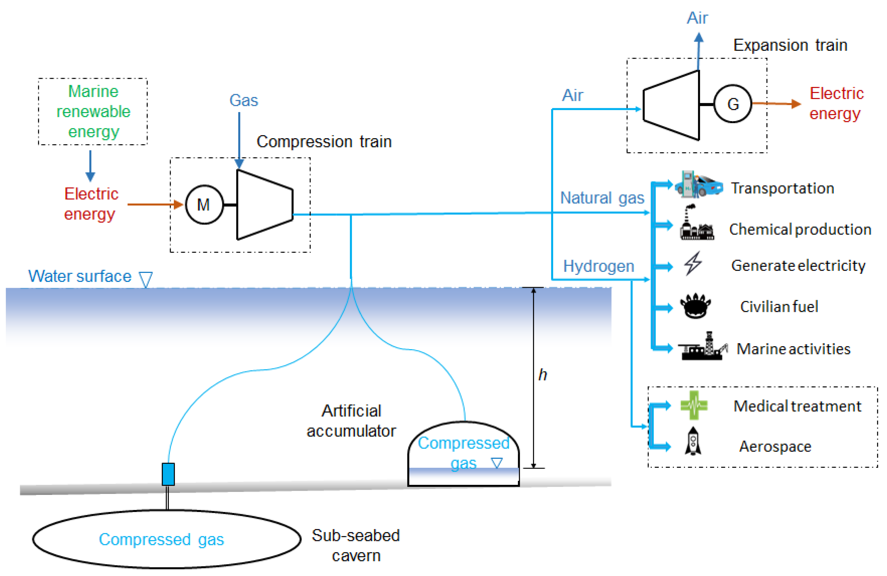
:1. Introduction
- Supersaturation of the gas inside the pipeline causes liquefaction and the formation of a liquid layer at the bottom.
- Temperature changes lead to the cooling of gas inside the pipeline, causing partial liquefaction and accumulation.
- Water is transported gas may react with cooled gas at the bottom of the pipeline, causing a liquid layer to form.
- High gas flow rates induce unstable gas movement, promoting localized pressure changes and the consequent liquefaction and accumulation of some gas at the pipeline bottom.
2. Experiment
2.1. Test Setup and Instrumentation
2.2. Experimental Process
3. OLGA Modeling
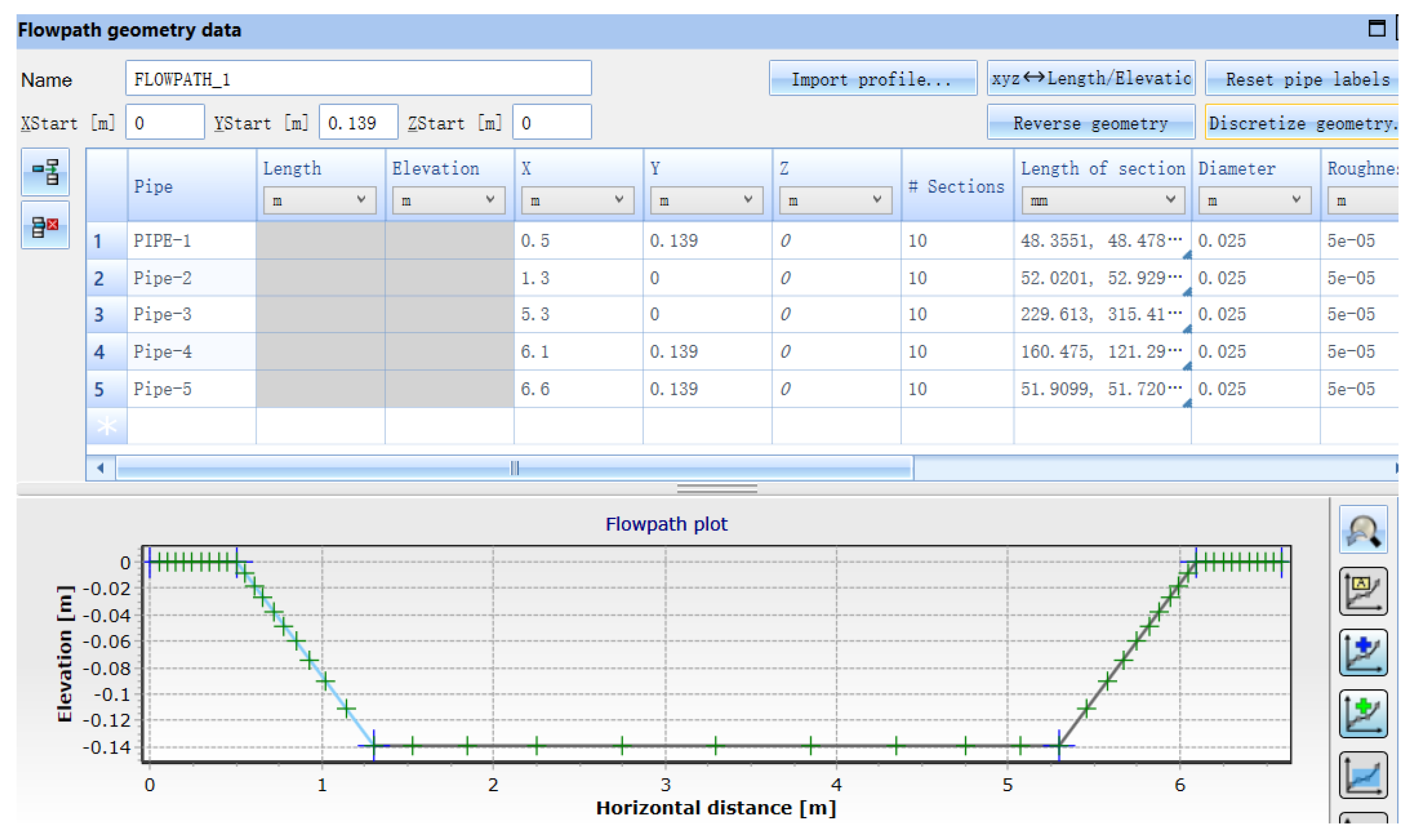
3.1. Pipeline Model
3.2. Fluids PVT Description
3.3. Boundary Conditions
4. Results and Discussion
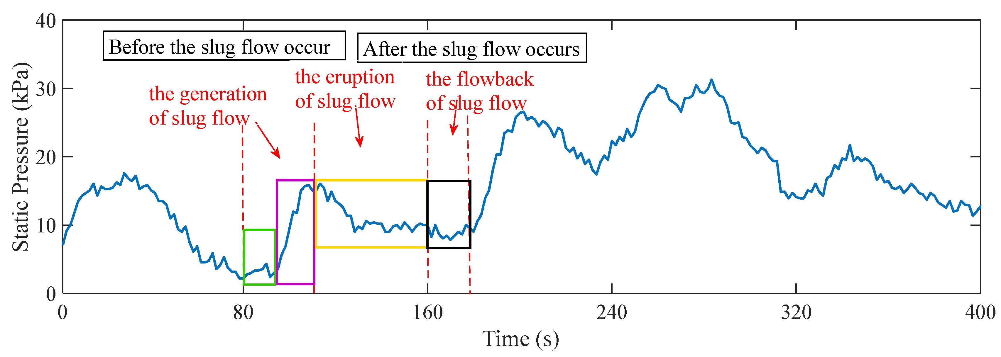
4.1. Experimental Results
4.2. Simulation Results and Comparisons
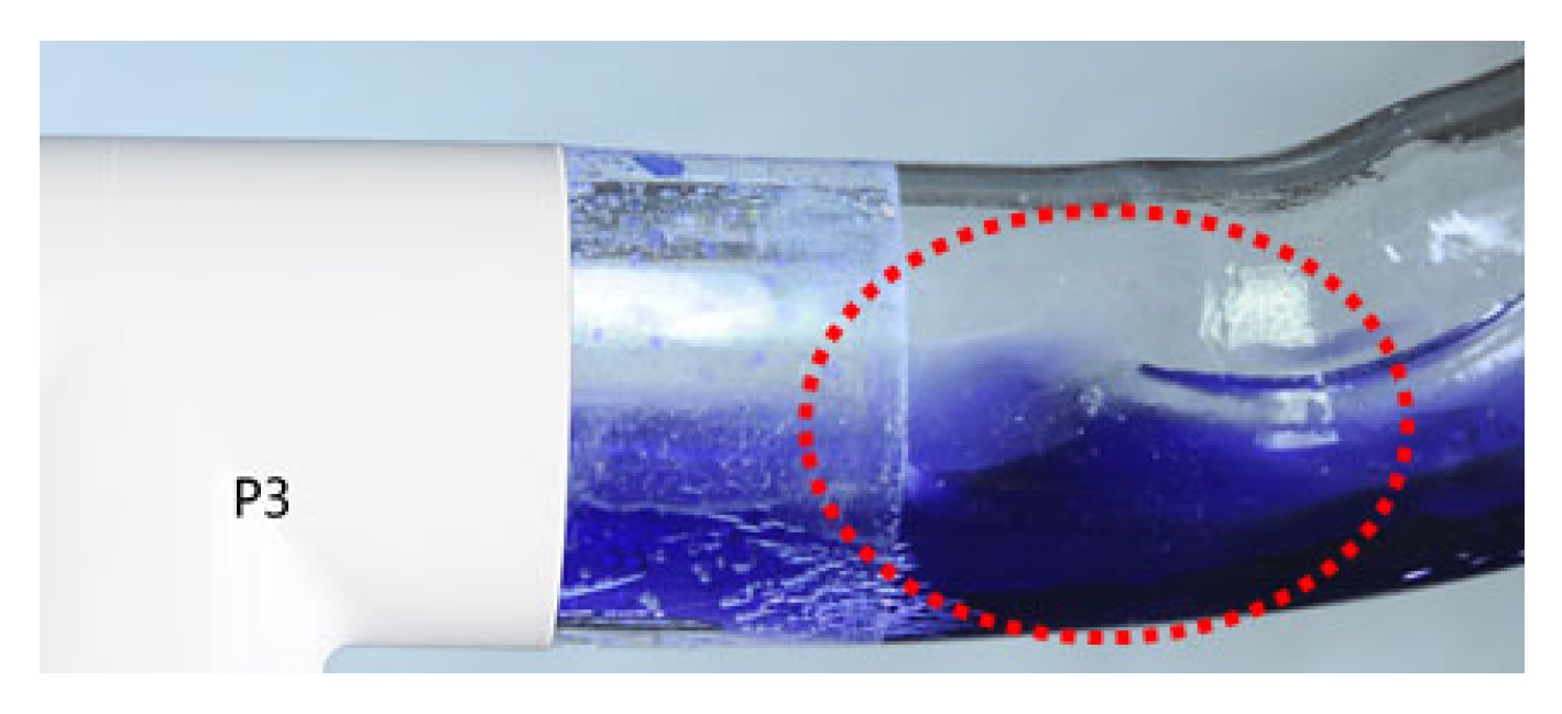
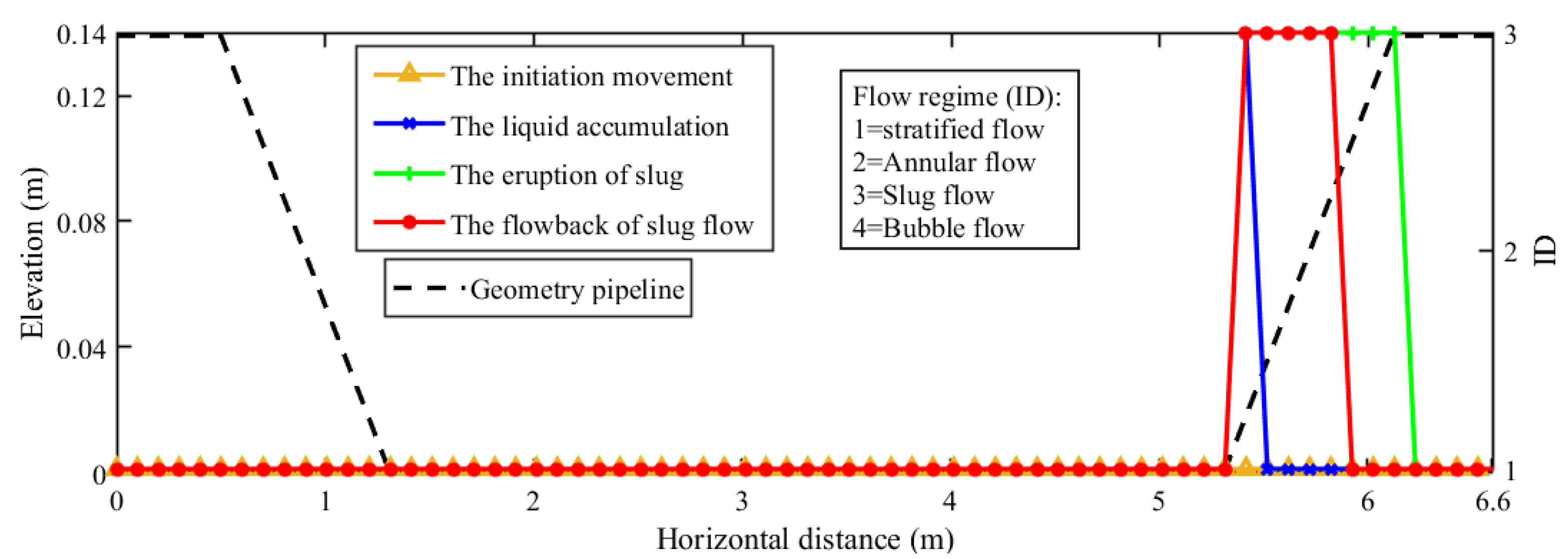
4.2.1. Flow Regime Analysis and Comparisons
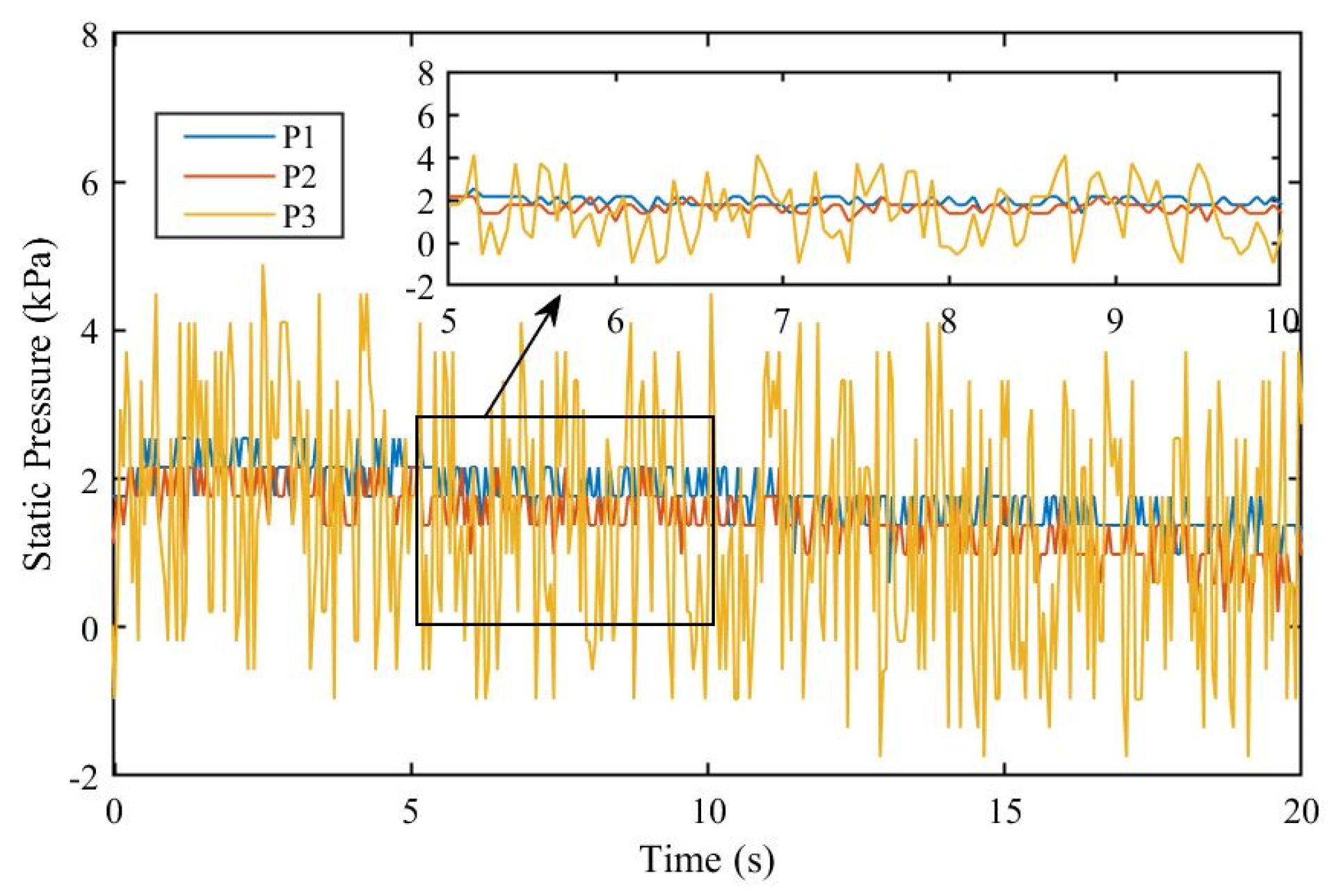
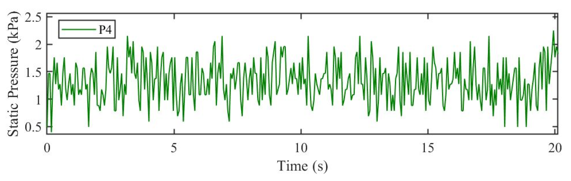
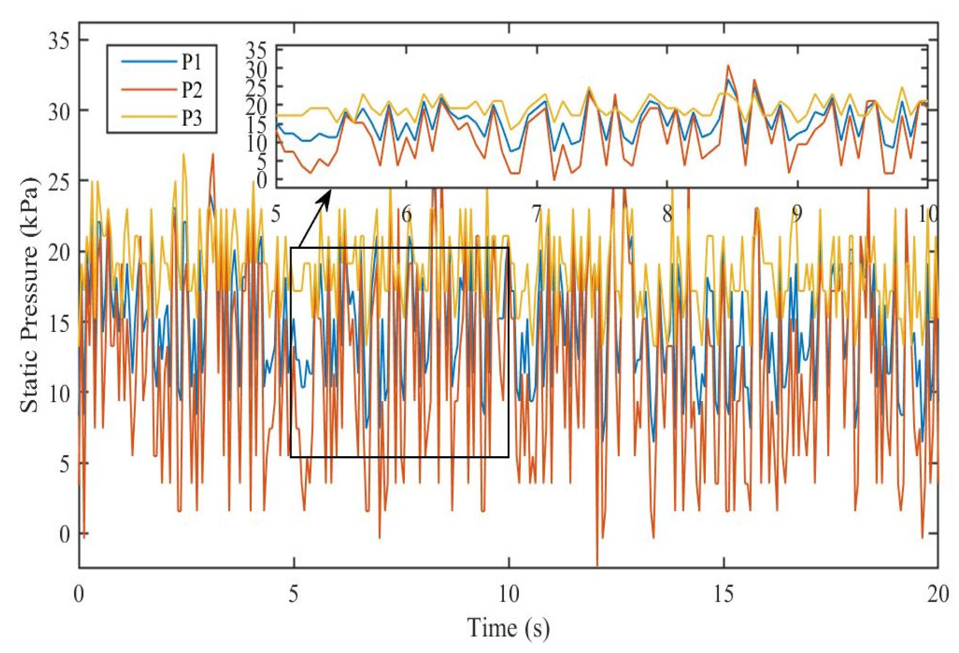
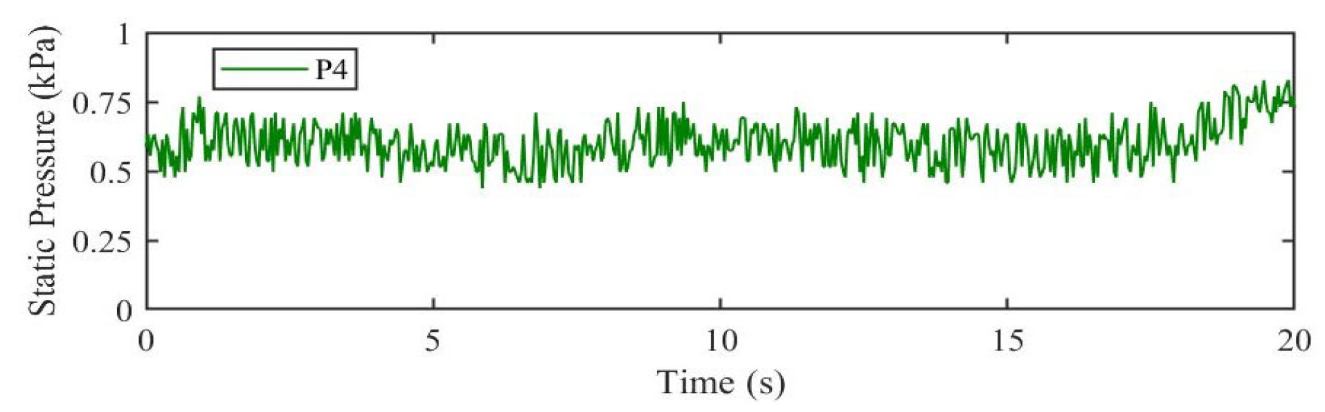
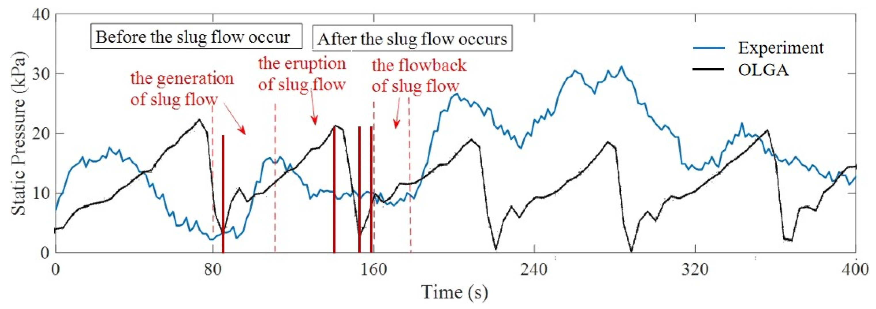
4.2.2. Pressure Analysis and Comparisons
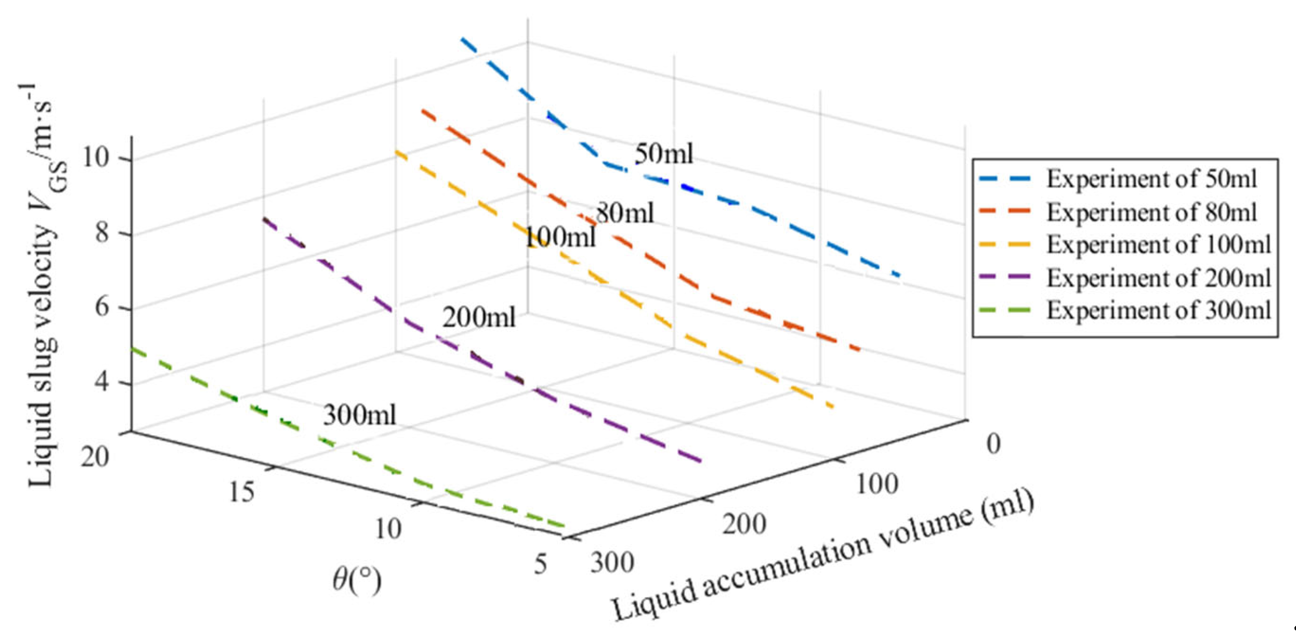
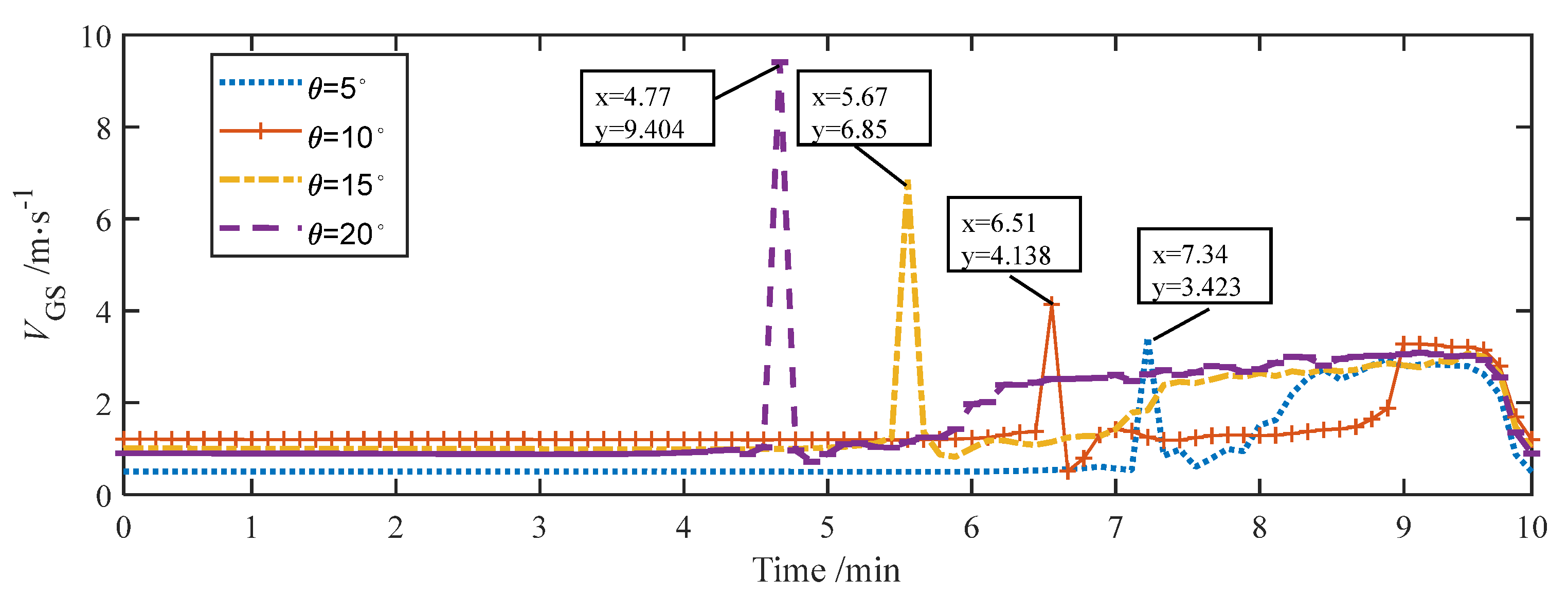
4.2.3. Gas Velocity Analysis and Comparisons
5. Conclusions
Author Contributions
Funding
Institutional Review Board Statement
Informed Consent Statement
Data Availability Statement
Conflicts of Interest
References
- Wang, H.; Wang, Z.; Liang, C.; Carriveau, R.; Ting, D.S.-K.; Li, P.; Cen, H.; Xiong, W. Underwater compressed gas energy storage (UWCGES): Current status, challenges, and future perspectives. Appl. Sci. 2022, 12, 9361. [Google Scholar] [CrossRef]
- Zhao, P.; Gou, F.; Xu, W.; Wang, J.; Dai, Y. Multi-objective optimization of a renewable power supply system with underwater compressed air energy storage for seawater reverse osmosis under two different operation schemes. Renew. Energy 2022, 181, 71–90. [Google Scholar] [CrossRef]
- Swinfen-Styles, L.; Garvey, S.D.; Giddings, D.; Cárdenas, B.; Rouse, J.P. Analysis of a Wind-Driven Air Compression System Utilising Underwater Compressed Air Energy Storage. Energies 2022, 15, 2142. [Google Scholar] [CrossRef]
- Anazi, A.A.A.; Barboza-Arenas, L.A.; Romero-Parra, R.M.; Sivaraman, R.; Qasim, M.T.; Al-Khafaji, S.H.; Gatea, M.A.; Alayi, R.; Farooq, W.; Jasiński, M. Investigation and Evaluation of the Hybrid System of Energy Storage for Renewable Energies. Energies 2023, 16, 2337. [Google Scholar] [CrossRef]
- Cárdenas, B.; Ibanez, R.; Rouse, J.; Swinfen-Styles, L.; Garvey, S. The effect of a nuclear baseload in a zero-carbon electricity system: An analysis for the UK. Renew. Energy 2023, 205, 256–272. [Google Scholar] [CrossRef]
- Jacobson, M.Z. NO MIRACLES NEEDED: How Today’s Technology Can Save Our Climate and Clean Our Air; Cambridge University Press: Cambridge, UK, 2023. [Google Scholar]
- Klyuev, M.; Schreider, A.; Rakitin, I. Technical Means for Underwater Archaeology; Springer Nature: Berlin/Heidelberg, Germany, 2023. [Google Scholar]
- Manakov, A.Y.; Stoporev, A.S. Physical chemistry and technological applications of gas hydrates: Topical aspects. Russ. Chem. Rev. 2021, 90, 566. [Google Scholar] [CrossRef]
- Zhang, S.-W.; Pan, Z.; Shang, L.-Y.; Zhou, L. Analysis of influencing factors on the kinetics characteristics of carbon dioxide hydrates in high pressure flow systems. Energy Fuels 2021, 35, 16241–16257. [Google Scholar] [CrossRef]
- Sun, H.; Chen, B.; Li, K.; Song, Y.; Yang, M.; Jiang, L.; Yan, J. Methane hydrate re-formation and blockage mechanism in a pore-level water-gas flow process. Energy 2023, 263, 125851. [Google Scholar] [CrossRef]
- Ramezani, L.; Karney, B.; Malekpour, A. Encouraging effective air management in water pipelines: A critical review. J. Water Resour. Plan. Manag. 2016, 142, 04016055. [Google Scholar] [CrossRef]
- Liang, C.; Xiong, W.; Wang, M.; Ting, D.S.; Carriveau, R.; Wang, Z. Experimental and Modeling Investigation for Slugging Pressure under Zero Net Liquid Flow in Underwater Compressed Gas Energy Storage Systems. Appl. Sci. 2023, 13, 1216. [Google Scholar] [CrossRef]
- Liang, C.; Xiong, W.; Carriveau, R.; Ting, D.S.; Wang, Z. Experimental and modeling investigation of critical slugging behavior in marine compressed gas energy storage systems. J. Energy Storage 2022, 49, 104038. [Google Scholar] [CrossRef]
- Duan, J.; Liu, H.; Tao, J.; Shen, T.; Hua, W.; Guan, J. Experimental Study on Gas–Liquid Interface Evolution during Liquid Displaced by Gas of Mobile Pipeline. Energies 2022, 15, 2489. [Google Scholar] [CrossRef]
- Zhang, S.-W.; Shang, L.-Y.; Zhou, L.; Lv, Z.-B. Hydrate deposition model and flow assurance technology in gas-dominant pipeline transportation systems: A review. Energy Fuels 2022, 36, 1747–1775. [Google Scholar] [CrossRef]
- Pektaş, M. Slug Flow Characterization in an Alkaline Water Electrolyzer for Hydrogen Production. Master’s Thesis, Delft University of Technology, Delft, The Netherland, 2023. [Google Scholar]
- Adouni, H.; Chouari, Y.; Bournot, H.; Kriaa, W.; Mhiri, H. A novel ventilation method to prevent obstruction phenomenon within sewer networks. Int. J. Heat Mass Transf. 2022, 184, 122335. [Google Scholar] [CrossRef]
- Li, Y.-L.; Ning, F.-L.; Xu, M.; Qi, M.-H.; Sun, J.-X.; Nouri, A.; Gao, D.-L.; Wu, N.-Y. Experimental study on solid particle migration and production behaviors during marine natural gas hydrate dissociation by depressurization. Pet. Sci. 2023. [Google Scholar] [CrossRef]
- Silva, M.; Campos, J.; Araújo, J. 3D numerical study of a single Taylor bubble rising along an inclined tube through Newtonian and non-Newtonian liquids. Chem. Eng. Process.-Process Intensif. 2023, 183, 109219. [Google Scholar] [CrossRef]
- Mousavi, S.M.; Sotoudeh, F.; Lee, B.J.; Paydari, M.-R.; Karimi, N. Effect of hybrid wall contact angles on slug flow behavior in a T-junction microchannel: A numerical study. Colloids Surf. A Physicochem. Eng. Asp. 2022, 650, 129677. [Google Scholar] [CrossRef]
- Lou, W.; Wang, Z.; Guo, B.; Pan, S.; Liu, Y.; Sun, B. Numerical analysis of velocity field and energy transformation, and prediction model for Taylor bubbles in annular slug flow of static power law fluid. Chem. Eng. Sci. 2022, 250, 117396. [Google Scholar] [CrossRef]
- Zhao, Y.; Lao, L.; Yeung, H. Investigation and prediction of slug flow characteristics in highly viscous liquid and gas flows in horizontal pipes. Chem. Eng. Res. Des. 2015, 102, 124–137. [Google Scholar] [CrossRef]
- Widyatama, A.; Venter, M.; Orejon, D.; Sefiane, K. Experimental investigation of bubble dynamics and flow patterns during flow boiling in high aspect ratio microchannels with the effect of flow orientation. Int. J. Therm. Sci. 2023, 189, 108238. [Google Scholar] [CrossRef]
- Titov, A.; Fan, Y.; Kutun, K.; Jin, G. Distributed Acoustic Sensing (DAS) Response of Rising Taylor Bubbles in Slug Flow. Sensors 2022, 22, 1266. [Google Scholar] [CrossRef] [PubMed]
- Amirsoleymani, A.; Ting, D.S.; Carriveau, R.; Brown, D.; McGillis, A. Two-phase flow pattern identification in CAES systems with dimensional analysis coupled with support vector machine. Int. J. Multiph. Flow 2023, 160, 104343. [Google Scholar] [CrossRef]
- Li, S.; Pei, H.; Liu, D.; Shen, Y.; Tao, X.; Gan, Z. Visualization study on the flow characteristics of a nitrogen pulsating heat pipe. Int. Commun. Heat Mass Transf. 2023, 143, 106722. [Google Scholar] [CrossRef]
- Munir, S.; Aziz, A.R.A.; Heikal, M.; Siddiqui, M.I. Combination of linear stochastic estimation and proper orthogonal decomposition: Application in two-phase slug flow. J. Braz. Soc. Mech. Sci. Eng. 2023, 45, 112. [Google Scholar] [CrossRef]
- Zhu, H.; Hu, J.; Gao, Y. Severe slug flow-induced nonlinear dynamic behavior of a flexible catenary riser. Phys. Fluids 2021, 33, 071705. [Google Scholar] [CrossRef]
- Zhu, H.; Gao, Y.; Zhao, H. Experimental investigation of slug flow-induced vibration of a flexible riser. Ocean Eng. 2019, 189, 106370. [Google Scholar] [CrossRef]
- Kim, H.-G.; Kim, S.-M. Experimental investigation of flow and pressure drop characteristics of air-oil slug flow in a horizontal tube. Int. J. Heat Mass Transf. 2022, 183, 122063. [Google Scholar] [CrossRef]
- Al-Dogail, A.S.; Gajbhiye, R.N. Effects of density, viscosity and surface tension on flow regimes and pressure drop of two-phase flow in horizontal pipes. J. Pet. Sci. Eng. 2021, 205, 108719. [Google Scholar] [CrossRef]
- Chen, J.; Luo, X.; He, L.; Liu, H.; Lu, L.; Lü, Y.; Yang, D. An improved solution to flow assurance in natural gas pipeline enabled by a novel self-regulated bypass pig prototype: An experimental and numerical study. J. Nat. Gas Sci. Eng. 2022, 107, 104776. [Google Scholar] [CrossRef]
- Lei, L.; Zhao, Y.; Wang, X.; Xin, G.; Zhang, J. Experimental and numerical studies of liquid-liquid slug flows in micro channels with Y-junction inlets. Chem. Eng. Sci. 2022, 252, 117289. [Google Scholar] [CrossRef]
- Wang, K.; Hu, C.; Cai, Y.; Li, Y.; Tang, D. Investigation of heat transfer and flow characteristics in two-phase loop thermosyphon by visualization experiments and CFD simulations. Int. J. Heat Mass Transf. 2023, 203, 123812. [Google Scholar] [CrossRef]
- Jiang, Y.; Zhang, Y.; Zhang, J.; Tang, Z. Characteristics of gas–liquid slug flow in honeycomb microchannel reactor. Energies 2022, 15, 1465. [Google Scholar] [CrossRef]
- Cao, X.; Zhang, P.; Li, X.; Li, Z.; Zhang, Q.; Bian, J. Experimental and numerical study on the flow characteristics of slug flow in a horizontal elbow. J. Pipeline Sci. Eng. 2022, 2, 100076. [Google Scholar] [CrossRef]
- Sergeev, V.; Vatin, N.; Kotov, E.; Nemova, D.; Khorobrov, S. Slug regime transitions in a two-phase flow in horizontal round pipe. CFD simulations. Appl. Sci. 2020, 10, 8739. [Google Scholar] [CrossRef]
- Valdés, J.P.; Pico, P.; Pereyra, E.; Ratkovich, N. Evaluation of drift-velocity closure relationships for highly viscous liquid-air slug flow in horizontal pipes through 3D CFD modelling. Chem. Eng. Sci. 2020, 217, 115537. [Google Scholar] [CrossRef]
- Pugliese, V.; Ettehadtavakkol, A.; Panacharoensawad, E. Drift flux model parameters estimation based on numerical simulation of slug flow regime with high-viscous liquids in pipelines. Int. J. Multiph. Flow 2021, 135, 103527. [Google Scholar] [CrossRef]
- Mesa, J.D.; Gao, H.; Constantinides, Y. Prediction and benchmarking of a nearly horizontal flowline slug flow. In Proceedings of the International Conference on Offshore Mechanics and Arctic Engineering, Hamburg, Germany, 5–10 June 2022; p. V007T008A023. [Google Scholar]
- Kim, S.; Yun, Y.; Choi, J.; Bizhani, M.; Kim, T.-w.; Jeong, H. Prediction of maximum slug length considering impact of well trajectories in British Columbia shale gas fields using machine learning. J. Nat. Gas Sci. Eng. 2022, 106, 104725. [Google Scholar] [CrossRef]
- Xiang, S.; Qin, Y.; Luo, J.; Pu, H.; Tang, B. Multicellular LSTM-based deep learning model for aero-engine remaining useful life prediction. Reliab. Eng. Syst. Saf. 2021, 216, 107927. [Google Scholar] [CrossRef]
- Ganat, T.; Hrairi, M. Effect of flow patterns on two-phase flow rate in vertical pipes. J. Adv. Res. Fluid Mech. Therm. Sci. 2019, 55, 150–160. [Google Scholar]
- Vandrangi, S.K.; Lemma, T.A.; Mujtaba, S.M.; Pedapati, S.R. Determination and analysis of leak estimation parameters in two-phase flow pipelines using OLGA multiphase software. Sustain. Comput. Inform. Syst. 2021, 31, 100564. [Google Scholar] [CrossRef]


| Water | Air | |
|---|---|---|
| Density | 997.05 kg∙m−3 | 1.184 kg∙m−3 |
| Kinetic Viscosity | 8.9008 × 10⁻⁴ Pa∙s | 1.849 × 10⁻⁵ Pa∙s |
| Surface Tension | Air/Water = 0.07197 N∙m−1 | |
| Component | Mole Fraction (%) | Density (kg∙m−3) |
|---|---|---|
| N2 | 78.126 | 1.184 |
| O2 | 20.907 | |
| Ar | 0.934 | |
| CO2 | 0.033 |
| Flow Model | Setting | |
|---|---|---|
| Overall setting | TEMPERATURE | WALL |
| STEADYSTATE | ON | |
| MASSEQCHEME | 1STORDER | |
| COMPOSITIONAL | OFF | |
| NOSLIP | OFF | |
| PHASE | THREE | |
| HYDSLUG | ON | |
| SLUGVOID | AIR | |
| TABLETOLERANCE | ON | |
| FLASHMODEL | WATER | |
| Integration | Simulation start time | 0 s |
| Simulation stop time | 30 min | |
| Minimum time step | 0.001 s | |
| Maximum time step | 0.5 s |
| Liquid Volume (mL) | Angle (°) | OLGA (m/s) | Experiment (m/s) | Error (%) |
|---|---|---|---|---|
| 50 | 5 | 5.51 | 5.72 | 3.81 |
| 10 | 6.29 | 6.11 | 2.86 | |
| 15 | 7.34 | 7.14 | 2.72 | |
| 20 | 9.73 | 10.65 | 9.45 | |
| 80 | 5 | 3.95 | 4.31 | 9.11 |
| 10 | 4.89 | 5.24 | 7.16 | |
| 15 | 7.09 | 6.88 | 2.96 | |
| 20 | 8.69 | 9.05 | 4.14 | |
| 100 | 5 | 3.75 | 4.02 | 7.2 |
| 10 | 4.61 | 4.98 | 8.03 | |
| 15 | 6.42 | 6.21 | 3.27 | |
| 20 | 7.89 | 8.13 | 3.04 | |
| 200 | 5 | 3.423 | 3.71 | 8.38 |
| 10 | 4.138 | 4.26 | 2.95 | |
| 15 | 6.85 | 5.79 | 15.47 | |
| 20 | 9.404 | 7.65 | 18.65 | |
| 300 | 5 | 2.56 | 2.34 | 8.59 |
| 10 | 3.04 | 2.91 | 4.28 | |
| 15 | 3.88 | 3.96 | 2.06 | |
| 20 | 4.91 | 5.12 | 4.27 |
Disclaimer/Publisher’s Note: The statements, opinions and data contained in all publications are solely those of the individual author(s) and contributor(s) and not of MDPI and/or the editor(s). MDPI and/or the editor(s) disclaim responsibility for any injury to people or property resulting from any ideas, methods, instructions or products referred to in the content. |
© 2023 by the authors. Licensee MDPI, Basel, Switzerland. This article is an open access article distributed under the terms and conditions of the Creative Commons Attribution (CC BY) license (https://creativecommons.org/licenses/by/4.0/).
Share and Cite
Liang, C.; Xiong, W.; Wang, H.; Wang, Z. Experimental and OLGA Modeling Investigation for Slugging in Underwater Compressed Gas Energy Storage Systems. Appl. Sci. 2023, 13, 9575. https://doi.org/10.3390/app13179575
Liang C, Xiong W, Wang H, Wang Z. Experimental and OLGA Modeling Investigation for Slugging in Underwater Compressed Gas Energy Storage Systems. Applied Sciences. 2023; 13(17):9575. https://doi.org/10.3390/app13179575
Chicago/Turabian StyleLiang, Chengyu, Wei Xiong, Hu Wang, and Zhiwen Wang. 2023. "Experimental and OLGA Modeling Investigation for Slugging in Underwater Compressed Gas Energy Storage Systems" Applied Sciences 13, no. 17: 9575. https://doi.org/10.3390/app13179575