Abstract
The goal of this paper is to analyze the optimal transfer towards the periodic comet 29P/Schwassmann–Wachmann 1 of a solar sail-based spacecraft. This periodic and active comet is an interesting and still unexplored small body that has been regarded as an object of the Centaurs group. In this work, a classical (heliocentric) orbit-to-orbit transfer is studied from an optimal viewpoint, by finding the spacecraft trajectories that minimize the flight time for a given value of the solar sail characteristic acceleration, that is, the typical performance parameter of a photonic sail. In particular, the optimal Earth–comet transfer is studied both in a typical three-dimensional mission scenario and with a simplified two-dimensional approach, whose aim is to rapidly obtain an accurate estimation of the minimum flight time with a reduced computation cost. The numerical simulations illustrate the mission performance, in terms of the characteristics of the rapid transfer trajectory, as a function of the typical propulsive parameter and the solar sail thrust model.
1. Introduction
This paper investigates the performance of a solar sail-based spacecraft in a classical, orbit-to-orbit, three-dimensional heliocentric transfer from Earth to comet 29P/ Schwassmann–Wachmann 1 (SW1) [1,2,3]. Comet SW1, which was discovered on 15 November 1927 by German astronomers Arnold Schwassmann and Arno Wachmann, currently covers a nearly circular orbit between Jupiter and Saturn with a small inclination to the Ecliptic [4], as sketched in Figure 1. This periodic and active comet, whose orbital period is roughly 15 years, is an interesting and still unexplored small body that has been regarded as an object of the Centaurs group [5,6,7], that is, a celestial body originating from the Kuiper belt and then moved to the inner region of the Solar System. Thanks to its (relative) accessibility if compared with the Kuiper belt objects, comet SW1 has been proposed as a potential target for a robotic exploration mission [8]. In particular, the aim of the proposed missions was both to obtain in situ physical measurements of such a primordial celestial body [9,10] and to collect the particles ejected by the comet during its frequent outbursts [11,12].
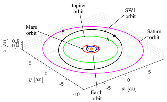
Figure 1.
Sketch of the comet SW1 heliocentric orbit evaluated at 1 August 2023. The figure shows, for comparison purposes, the orbits of Mars, Earth, Jupiter, and Saturn. The star symbol indicates the perihelion point of the generic heliocentric orbit.
In this paper, the capability of a spacecraft equipped with a photonic solar sail to perform a rendezvous of the SW1 orbit is investigated from an optimal viewpoint. In fact, the specific characteristics of the SW1 heliocentric orbit, which can be roughly approximated with a circular orbit of radius , make the solar sail transfer a challenging problem, due to the fact that the maximum magnitude of the sail propulsive acceleration is inversely proportional to the square of the solar distance. Accordingly, and as also highlighted in the next section, just before the cometary rendezvous the propellantless propulsion system can give only a small fraction (about ) of the total thrust available just after the launch from the Earth, that is, when the Sun–spacecraft distance is roughly . Indeed, a solar sail-based propulsion system is rarely considered in a heliocentric mission scenario which requires the thrust vectoring at a solar distance greater than , that is, beyond the typical Jupiter distance from the Sun. However, the photonic solar sail can be still effective even beyond a radial distance of , as highlighted by the numerical results discussed later in this paper.
In fact, the (rather) common assumption that a solar sail should be jettisoned, or the solar sail-induced propulsive acceleration should be neglected, when the solar distance is greater than , originates from the interesting work by Carl Sauer [13] that analyzes the photonic solar sail performance in a Solar System escape (more precisely, the term used in [13] is ‘interstellar’) mission scenario. In particular, according to [13], in the last paragraph of p. 9 Sauer substantially affirms that “...the effectiveness of the sail in reducing flight time is minimal...” when the solar distance of the spacecraft is in the range , so that the primary propulsion system (i.e., the solar sail) is jettisoned at “...to allow the acquisition of science data without possible interference from the sail”. This conclusion is, indeed, absolutely acceptable in a Solar System escape trajectory such as that analyzed in the second part of [13], because such a specific trajectory uses a pass close to the Sun (i.e., a sort of ‘solar photonic assist maneuver’ as named by Leipold and Wagner [14] and Dachwald [15] in their fine paper of 2004) to reach the required value of the hyperbolic excess speed. On the other hand, in a Solar System escape scenario the use of a solar sail-based propulsion system at a distance greater than is still possible, but the reduction in the total flight time (in that case, the flight times are of the order of decades) is marginal when compared to the increase in difficulty to actively change the sail attitude at such great solar distances.
Bearing in mind that a rendezvous with the active comet SW1 is therefore a challenging scenario for a (photonic) solar sail-based spacecraft, this work aims to illustrate the results of a preliminary, orbit-to-orbit, heliocentric trajectory design by considering the (simplified) thrust vector that models the performance of a flat sail of assigned characteristics. In this context, the paper takes advantage of both the analytical model and the ad hoc automatic routines already implemented by the authors to study this specific mission scenario. In this sense, the contribution of this work is not to propose new optimization techniques or to refine the mathematical model for the solar sail-based trajectory design, but to collect and comment on the results of a simulation campaign aimed at estimating the potentialities of such a propellantless propulsion system in a challenging mission scenario such as the rendezvous with the comet SW1.
In particular, taking the actual characteristics of the Earth and SW1 heliocentric orbits into account, the minimum flight time is evaluated by considering both an ideal force model (i.e., a model in which the sail is assumed as a flat, perfectly reflecting, mirror) and an optical force model (i.e., a model in which the thermo-optical characteristics of the reflecting film are taken into account) to describe the solar sail thrust vector during the deep space flight [16,17]. The numerical analysis presents a parametric study of the transfer time as a function of the sail typical performance parameter, i.e., the characteristic acceleration [18] defined as the maximum magnitude of the sail propulsive acceleration vector at a distance of 1 astronomical unit from the Sun.
Finally, the numerical results obtained through a simplified, but less computationally demanding, two-dimensional approach to the preliminary trajectory design are discussed in the last part of the work. In this context, bearing in mind the orbital characteristics (i.e., the value of the eccentricity and the inclination) of both the starting (Earth) and target (SW1) orbit, the spacecraft heliocentric transfer is approximated through a classical circle-to-circle orbit raising [19] and the mission performance is obtained by using the typical approach discussed in the recent literature [20]. The numerical simulations will show that, even with a non-negligible value of the target orbit inclination over the Ecliptic (the value of that orbital inclination is about 9 degrees), the two-dimensional circle-to-circle approximation of the orbit transfer gives both a flight time and a shape of the transfer trajectory which are very close to those obtained with a three-dimensional approach.
The paper is organized as follows. Section 2 briefly describes the mathematical model, that is, the three-dimensional spacecraft dynamics and the (rather classical) procedure which has been used to optimize the spacecraft trajectory during the interplanetary transfer. In particular, the aim of Section 2 is only to illustrates the main features of the mathematical model that, in its turn, has already been commented on in detail by the authors in the suggested references. Section 3 discusses the results of numerical simulations, in terms of a parametric study of the mission performance (i.e., the minimum flight time) as a function of the solar sail propulsive characteristics, and the results of a case study which refers to a specific value of the sail (reference) propulsive acceleration. A two-dimensional approach to the optimal trajectory design is then proposed in Section 4, whose aim is to obtain an approximate value of the optimal flight time with a reduced computation time. Finally, the concluding remarks are drawn in Section 5, as usual.
2. Mathematical Preliminaries and Models
The problem addressed in this section is to analyze the rapid transfer trajectory, in a three-dimensional heliocentric mission scenario, of a spacecraft whose primary propulsion system is a classical (photonic) solar sail of assigned characteristics. In this context, assume that the solar sail-based spacecraft initially (i.e., at time ) covers a Keplerian (three-dimensional) orbit which coincides with the Earth’s orbit around the Sun, whose gravitational parameter is . As is well known, such a specific scenario is consistent with a solar sail deployment just outside the Earth’s sphere of influence [21], when the spacecraft leaves the planet using a Keplerian parabolic escape trajectory.
In an orbit-to-orbit transfer, the spacecraft uses the propulsive acceleration given by the solar sail propulsion system to reach, at time , a Keplerian orbit which coincides with the SW1 heliocentric trajectory. According to the common assumptions used in the preliminary phase of the trajectory design, during the transfer, that is, during the time interval , the spacecraft is subjected to the Sun’s gravitational acceleration and, possibly, solar sail-induced thrust. Moreover, in an orbit-to-orbit transfer the initial (or final) angular position of the spacecraft along the parking (or target) orbit is left free, so that the initial (or final) spacecraft true anomaly (or ) is obtained as an output of a trajectory optimization process that extremizes (i.e., optimizes) a given performance index. On the other hand, the remaining classical orbital parameters that define the parking (i.e., the Earth) and the target (i.e., the comet SW1) orbit are considered assigned, and they are reassumed in Table 1. In particular, this table gives the value of the semimajor axis a, eccentricity e, orbital inclination i, argument of perihelion , and right ascension of the ascending node , which are obtained through the well known JPL Horizons system.

Table 1.
Classical orbital elements of the parking (Earth) and target (comet SW1) orbit used in the numerical simulations.
Note that the comet SW1 orbital elements reassumed in Table 1 are evaluated at the beginning of August 2023. In fact, as discussed by Sarid et al. [22], the heliocentric orbit of comet SW1 is (strongly) perturbed by Jupiter’s gravitational attraction, and the simulations show that the Jupiter conjunction of year 2038 will (roughly) double the eccentricity of the comet orbit.
In a solar sail-based mission scenario, the time variation of the thrust vector components is typically calculated by minimizing the total flight time [23], that is, by studying the (rapid) transfer trajectory which maximizes the performance index J defined as
The procedure used in this work to maximize the performance index J and, then, to obtain the minimum flight time related to the rapid transfer trajectory, has already been validated in a number of different mission scenarios which involve the solar sail-based spacecraft transfer towards Solar System small bodies, as also illustrated in some recent authors’ works [24,25]. An interesting approach to the solar sail-based trajectory optimization, in missions toward Solar System small bodies, is also discussed in the works by Heiligers et al. [26] and Zeng et al. [27]. In particular, the procedure used in this work will be (briefly) illustrated at the end of this section, for the sake of completeness. The next subsection, instead, illustrates the mathematical model used to describe the solar sail-based spacecraft dynamics in the three-dimensional heliocentric scenario.
2.1. Spacecraft Dynamics
Paralleling the approach employed by the authors in the recent literature [25], the motion of the solar sail-based spacecraft during the heliocentric transfer is described using the modified equinoctial elements (MEOEs) introduced by Walker in 1985 [28,29]. In particular, MEOEs are elements valid for a generic osculating orbit, which are related to the classical orbital elements through the simple relationships [28,29]
while the inverse passage is obtained by using the equations
Note that p is the semilatus rectum of the spacecraft osculating orbit, see the first of Equation (2), while the true longitude L is the fast varying variable which indicates the spacecraft angular position along the transfer orbit; see the last of Equation (2).
According to Betts [30], if one defines the spacecraft state vector as
the spacecraft dynamics can be described by the following (compact) differential vectorial equation
where is the solar sail-induced propulsive acceleration vector, while and are defined as
The six scalar initial conditions associated with the vectorial differential Equation (10) model the spacecraft motion along the Earth’s heliocentric orbit at time . Bearing in mind that in an orbit-to-orbit transfer the (initial) spacecraft angular position is left free, one obtains five initial conditions by combining Equation (2) and the data of the first row of Table 1. In that case, and according to [25], the result is given by the following equations
The three components of vector which appear in Equation (10) coincide with the components of the propulsive acceleration vector in a typical radial–tangential–normal (RTN) reference frame of unit vectors . In particular, the RTN reference frame is sketched in Figure 2, in which is the Sun–spacecraft vector and is the radial unit vector, where r is the Sun–spacecraft distance. Note that , the plane coincides with the plane of the osculating orbit, and the normal unit vector is aligned with the spacecraft specific angular momentum vector.
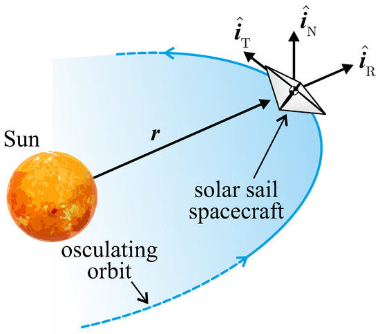
Figure 2.
Typical RTN reference frame and characteristics of the spacecraft osculating orbit.
The analytical expression of the components of in the RTN reference frame depends on the solar sail thrust model which is adopted to describe the propulsive performance of such a propellantless thruster. In this context, assuming a flat sail, i.e., a solar sail with a rigid and flat reflecting membrane, a common choice in the preliminary trajectory design is to use the optical force model without degradation [31,32]. The interested reader should note that the solar sail thrust vector can be described through a more refined (and complex) mathematical model. In this sense, the work of Vulpetti [33], which can be considered one of the founders of the photonic solar sail astrodynamics, discusses the effect of wrinkles on the thrust vector characteristics. The optical force model, which is detailed in the classical McInnes’ textbook [34], allows the propulsive acceleration vector to be written, in a compact analytical form, as a function of the radial unit vector and the normal unit vector , which is defined as the unit vector normal to the sail (nominal) plane in the direction opposite to the Sun [18,34]. Bearing in mind the approach described in [35], the compact expression of the propulsive acceleration vector is
where is a reference distance, is the characteristic acceleration defined as the propulsive acceleration magnitude experienced by a solar sail whose reference plane is oriented perpendicular to the solar rays when , and are dimensionless (normalized) force coefficients where , whose value depends on the optical characteristics of the reflecting membrane. In particular, assuming a membrane with a highly reflective aluminum-coated front side and a highly emissive chromium-coated back side [36], the values of the normalized force coefficients are reassumed in Table 2, which also details the values of for an ideal force model [25].
Table 2.
Normalized force coefficients for an ideal and an optical force model, assuming a (rigid and flat) sail membrane with a highly reflective aluminum-coated front side and a highly emissive chromium-coated back side.
Note that the term is the common solar sail performance parameter, whose value depends on the characteristics of both the solar sail and the whole spacecraft (including the value of the payload mass and other subsystems). For example, the upcoming NASA’s Solar Cruiser demonstration mission [37] has a characteristic acceleration of about . Moreover, in Equation (14) the normal unit vector is the control term in the trajectory design, that is, bearing in mind the natural constraint , one has two independent scalar control variables in the optimization problem, which is briefly described in the next subsection.
2.2. Trajectory Optimization
Fon an assigned value of the characteristic acceleration , the optimal orbit-to-orbit transfer has been studied using an indirect approach [38] in which the Hamiltonian function is obtained from Equation (10) as [25]
where is the adjoint vector [39]. The time derivative of is given by the classical Euler–Lagrange equations
which gives six first-order, non-linear, differential equation in the variables , whose explicit expressions are omitted here for the sake of brevity.
During the transfer, the optimal control vector, that is, the optimal sail attitude in terms of time variation of , is obtained by using Pontryagin’s maximum principle, that is, by finding the value of the normal unit vector that maximizes (at any time) the Hamiltonian function given by Equation (15). In this respect, a numerical approach is used to calculate the two (independent) scalar variables that maximize the value of and the procedure is illustrated in the recent authors’ work [25].
The equations of motion (10) and the Euler–Lagrange Equation (16) form the two-point boundary problem (TPBVP) which is completed by 13 boundary conditions, because the (optimal) flight time is an output of the optimization process. In particular, five (initial) conditions are given by Equation (13), while five (final) conditions are obtained by enforcing the rendezvous with comet SW1 orbit. In this respect, using the data from Table 1 and Equation (2), one obtains
Finally, the last three scalar constraints required to complete the TPBVP are obtained from the transversality condition [39] as
The TPBVP has been solved using an in-house procedure based on the multiple shooting method and the use of genetic algorithms. In particular, the differential equations have been integrated in double precision using a variable order Adams–Bashforth–Moulton solver [40] with absolute and relative errors of . The results of this numerical optimization process are illustrated in the next section, which contains both a parametric analysis of the orbit-to-orbit transfer as a function of the value of the characteristic acceleration and a detailed case study for a specific value of .
3. Numerical Simulations
The optimization procedure discussed in the previous section has been applied to evaluate the rapid Earth–comet SW1 transfer as a function of the spacecraft characteristic acceleration value in the range , with a step of ; see the red circles in Figure 3 for example.
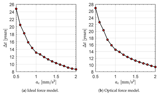
Figure 3.
Minimum flight time as a function of the spacecraft characteristic acceleration , in an Earth–comet SW1 orbit-to-orbit transfer using an ideal or optical force model.
Bearing in mind the current solar sail technology level [16,23], the range below the (usually considered as canonical [34]) value of is consistent with a medium–high performance solar sail, which hopefully will be available in the near future. On the other hand, the upper part of the selected range of models the behavior of a (more futuristic) high performance sail [41,42,43,44], which uses advanced materials [45,46] to improve the propulsive performance. In order to evaluate the impact on the transfer performance of the sail thrust characterization, the orbit-to-orbit transfer has been optimized by considering both the ideal and the optical force model, using the normalized coefficients reassumed in Table 2. The results, in terms of optimal flight time as a function of , are given by Figure 3 for the two force models.
Figure 3 clearly shows that the (optimal) flight time of a medium–high performance solar sail is well above 10 years, with a value of when for both the force models considered in the numerical simulations. On the other hand, an orbit-to-orbit transfer time below 10 years can be reached only through a high performance solar sail. In this context, for example, a sail with is required when an optical force model is used to describe the thrust vector. This aspect is due to the combination of a high value of the semimajor axis and a low eccentricity of the comet SW1 heliocentric orbit, which gives a perihelion (or aphelion) distance of about (or ). In fact, a classical solar sail is quite ineffective at such distances from the Sun, because the maximum magnitude of the solar sail propulsive acceleration varies as , as described by Equation (14). In this specific mission scenario one obtains that the dimensionless ratio is in the range when the spacecraft completes the rendezvous, as illustrated by the curve of Figure 4, which describes the variation of the ratio as a function of the spacecraft (final) true anomaly along the comet orbit. In other terms, at the end of the mission the solar sail-induced propulsive acceleration magnitude is only a small fraction (i.e., a value below ) of the initial maximum value, which roughly coincides with by construction.
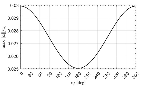
Figure 4.
Variation of the dimensionless ratio as a function of the spacecraft (final) true anomaly .
The numerical simulations show that the spacecraft with a medium–high performance solar sail completes several revolutions during the optimal orbit-to-orbit transfer. This point is highlighted by Figure 5, which shows the variation in true longitude during the transfer. Note that the integer part of the ratio indicates the revolutions around the Sun completed by the spacecraft before reaching the comet SW1 heliocentric orbit. The value of is consistent with the curves reassumed in Figure 6, which shows the ecliptic projection of the optimal transfer trajectory for some values of , using an optical force model.
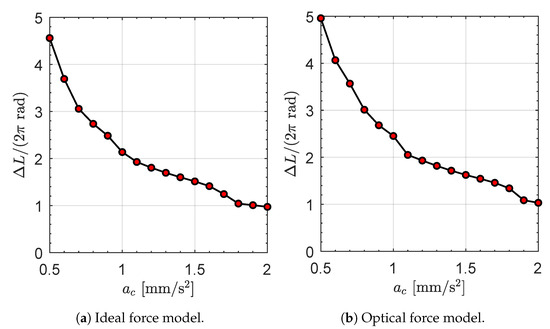
Figure 5.
Variation in true longitude during the optimal transfer, as a function of the characteristic acceleration and force model.
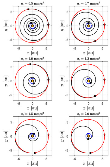
Figure 6.
Ecliptic projection of the optimal transfer trajectory (black line) for an optical force model, when . Black circle → start; square → arrival; star → perihelion point; orange circle → Sun; blue line → Earth’s orbit; red line → comet SW1 orbit.
Figure 3 also shows, as expected, that the performance of the ideal force model (in terms of flight time) is better than that obtained through an optical force model. However, the relative difference between the (minimum) flight time obtained through the two force models is below , as highlighted in Figure 7.

Figure 7.
Comparison between the minimum flight time obtained with an ideal () and an optical () force model as a function of the characteristic acceleration .
The numerical solution of the TPBVP gives, as secondary outputs, the (optimal) value of the true anomaly both at the beginning () and the end () of the transfer, as sketched in Figure 8. Note that the value of the pair is useful to find a launch window for the rapid transfer, as a function of the value of the characteristic acceleration.

Figure 8.
Initial and final true anomaly in a rapid transfer using an ideal or optical force model.
Case Study
This subsection gives a detailed calculation of the characteristics of the optimal transfer trajectory for specific value of . In this context, the (canonical) value of has been selected to describe the time variation of both the spacecraft osculating orbital parameters and the sail attitude during the orbit-to-orbit transfer. In this case, the optimal flight time is , that is, about ; see also Figure 3b. The time variation of the classical orbital parameters of the spacecraft osculating orbit is shown in Figure 9, where one can observe that the change in orbital inclination is substantially performed in the first part of the transfer, that is, when the Sun–spacecraft distance is still in the order of one astronomical unit. The sketch of the optimal transfer is reported in Figure 10.
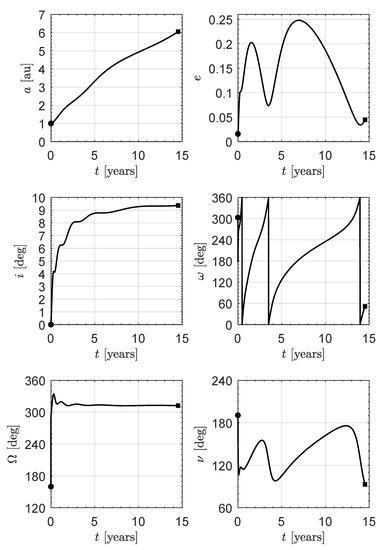
Figure 9.
Time variation of the spacecraft osculating orbit elements during the optimal transfer with and an optical force model. Circle → start; square → arrival.
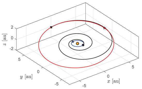
Figure 10.
Optimal transfer trajectory (black line) for an optical force model, when . Black circle → start; square → arrival; star → perihelion; orange circle → Sun; blue line → Earth’s orbit; red line → comet SW1 orbit.
Finally, the optimal control law, in terms of the time variation of the component of the normal unit vector in the RTN reference frame, is reported in Figure 11. Note that the three components of are roughly constant for , that is, the sail attitude (with respect to the RTN reference frame) is nearly fixed for about of the transfer. In particular, such an attitude maximizes the transverse component (i.e., the component perpendicular to the radial direction) of the propulsive acceleration . This is an interesting result, which is consistent with the model described in the next section, where a two-dimensional approach is used to obtain an accurate approximation of the optimal transfer performance with a reduced computation time.
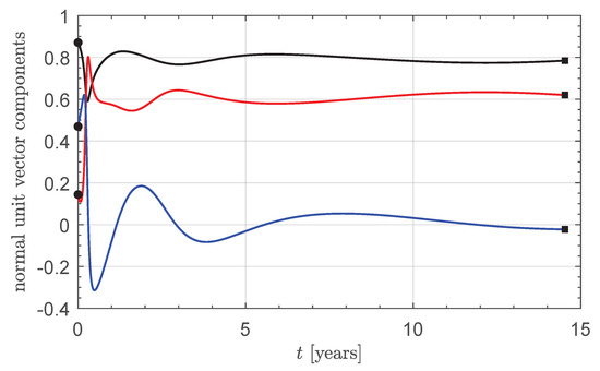
Figure 11.
Time variation of the components of the normal unit vector (in the RTN reference frame) during the optimal transfer with and an optical force model. Circle → start; square → arrival; black line → radial component; red line → tangential component; blue line → normal component.
4. Two-Dimensional Simplified Approach
The (very) small value of the eccentricity of both the Earth and comet SW1 heliocentric orbit, together with the small relative orbital inclination (slightly above , see data in Table 1), suggest the use of a simplified mathematical model to study the optimal orbit-to-orbit transfer. In fact, an Earth–comet SW1 mission is the typical scenario that can be approximated through a classical circle-to-circle orbit raising, in which the celestial bodies’ (heliocentric) orbits are assumed as circular and coplanar. In that case, the spacecraft dynamics can be described with a (simplified) mathematical model which uses the classical spacecraft equations of motion in the polar (heliocentric) reference frame sketched in Figure 12. In this respect, the dynamics model and the optimization procedure are thoroughly described (and commented on) in a number of the authors’ works [19,47], and they are omitted here for the sake of brevity.
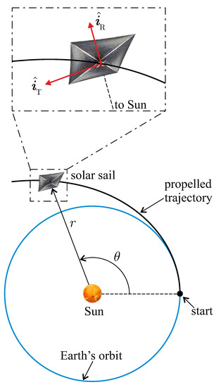
Figure 12.
Heliocentric polar reference frame and polar angle .
In particular, the radius of the initial (or final) circular orbit is assumed as (or , i.e., a value that coincides with the semimajor axis of the comet SW1 orbit), while the initial polar angle is set to for symmetry reasons; see Figure 12. Using such a two-dimensional approach to trajectory optimization, and considering the range of characteristic acceleration , the minimum flight time for an ideal or optical force model has been reassumed in Figure 13 as a function of . A comparison between the curves of Figure 13 and that of Figure 3 (which refer to a complete three-dimensional scenario), indicates that the results obtained through a two-dimensional approach approximate very well the values obtained with a more realistic model. This aspect is confirmed by Figure 14, which shows that the percentage difference between the minimum flight time obtained through a three-dimensional () and a two-dimensional () approach is below for both the two force models.

Figure 13.
Minimum flight time as a function of the spacecraft characteristic acceleration , for an Earth–comet SW1 circle-to-circle (coplanar) two-dimensional orbit raising.
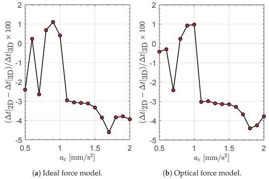
Figure 14.
Comparison between the minimum flight time obtained with a three-dimensional () and a two-dimensional () approach to trajectory optimization.
The solution of the optimal control problem also gives the value of the final polar angle , which can be used to evaluate the number of complete revolutions around the Sun during the transfer. In this case, the numerical results are reassumed in Figure 15, while Figure 16 shows a set of optimal transfer trajectories (in polar form), when an optical force model is considered in the simulations. Bearing in mind that , one observes that the trajectories of Figure 16 are consistent (and in some cases substantially coincident) with the trajectories reported in Figure 6. This is an important result, because it confirms a posteriori the usefulness of the two-dimensional approach, which requires a computation time of about two orders of magnitude less than that related to the three-dimensional model.
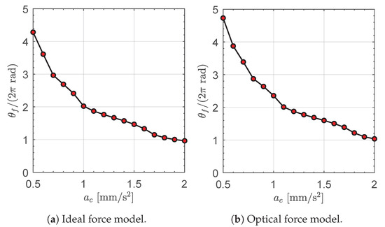
Figure 15.
Final polar angle as a function of the spacecraft characteristic acceleration , for an Earth–comet SW1 circle-to-circle (coplanar) two-dimensional orbit raising.
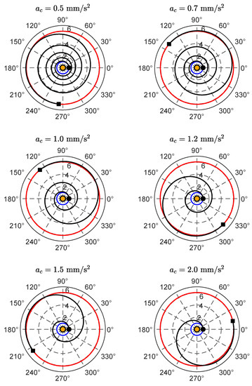
Figure 16.
Polar form of the optimal transfer trajectory (black line) for an optical force model, when . Black circle → start; square → arrival; orange circle → Sun; blue line → Earth’s orbit; red line → comet SW1 orbit.
5. Conclusions
A solar sail-based rendezvous with comet 29P/Schwassmann–Wachmann 1 requires a flight time of about two decades when a medium–high performance sail is considered in the orbital simulations. Accordingly, such a complex mission scenario can be considered a typical application of a high performance sail, which could give a flight time less than ten years, even with a realistic optical force model. In this respect, the numerical results discussed in this paper can be used to obtain a fast estimation of the characteristics of the optimal transfer trajectory with a reduced computation time. A possible extension of this work is to consider a cometary flyby mission, instead of a rendezvous scenario, in order to reduce the required flight time for a given value of the characteristic acceleration. In fact, a flyby mission has a less constrained terminal condition, so that the flight time is surely lesser than the time obtained in the paper. Accordingly, for example, if the scientific mission requires a cometary flyby and not an in situ study, the flight time can be significantly less than the decades obtained in the previous section, the value of the characteristic acceleration being the same.
Author Contributions
Conceptualization, A.A.Q.; methodology, A.A.Q.; software, A.A.Q.; writing—original draft preparation, A.A.Q.; writing—review and editing, A.A.Q., K.A.S., and G.P. All authors have read and agreed to the published version of the manuscript.
Funding
This research received no external funding.
Institutional Review Board Statement
Not applicable.
Informed Consent Statement
Not applicable.
Data Availability Statement
Not applicable.
Conflicts of Interest
The authors declare no conflict of interest.
Abbreviations
| JPL | Jet Propulsion Laboratory |
| MEOE | modified equinoctial element |
| RTN | radial–tangential–normal |
| SW1 | 29P/Schwassmann–Wachmann 1 |
| TPBVP | two-point boundary problem |
| a | semimajor axis [au] |
| characteristic acceleration [mm/s] | |
| propulsive acceleration vector [mm/s] | |
| matrix, see Equation (11) | |
| force coefficients, see Table 2 | |
| vector, see Equation (11) | |
| e | eccentricity |
| Hamiltonian function | |
| i | orbital inclination [deg] |
| radial unit vector | |
| transverse unit vector | |
| normal unit vector | |
| J | performance index [days] |
| normal unit vector | |
| MEOEs | |
| r | Sun–spacecraft distance [au] |
| position vector [au] | |
| Sun–spacecraft unit vector | |
| reference distance [] | |
| t | time [days] |
| spacecraft state vector | |
| flight time [days] | |
| adjoint vector | |
| generic adjoint variable | |
| Sun’s gravitational parameter [km/s] | |
| argument of periapse [deg] | |
| right ascension of the ascending node [deg] | |
| Subscripts | |
| 0 | initial, Earth’s heliocentric orbit |
| f | final, comet SW1 heliocentric orbit |
| Superscripts | |
| · | derivative with respect to time |
References
- Gunnarsson, M.; Rickman, H.; Festou, M.; Winnberg, A.; Tancredi, G. An extended CO source around comet 29P/Schwassmann-Wachmann 1. Icarus 2002, 157, 309–322. [Google Scholar] [CrossRef]
- Gronkowski, P. Cometary outbursts—Search of probable mechanisms—Case of 29P/Schwassmann-Wachmann 1. Astron. Nachr. 2002, 323, 49–56. [Google Scholar] [CrossRef]
- Stansberry, J.; Van Cleve, J.; Reach, W.; Cruikshank, D.; Emery, J.; Fernandez, Y.; Meadows, V.; Su, K.; Misselt, K.; Rieke, G.; et al. Spitzer observations of the dust coma and nucleus of 29P/Schwassmann-Wachmann. Astrophys. J. Suppl. Ser. 2004, 154, 463–468. [Google Scholar] [CrossRef]
- Neslusan, L.; Tomko, D.; Ivanova, O. On the chaotic orbit of comet 29P/Schwassmann-Wachmann 1. Contrib. Astron. Obs. Skaln. Pleso 2017, 47, 7–18. [Google Scholar]
- Kokhirova, G.; Ivanova, O.; Rakhmatullaeva, F.D.; Buriev, A.; Khamroev, U. Astrometric and photometric observations of comet 29P/Schwassmann-Wachmann 1 at the Sanglokh international astronomical observatory. Planet. Space Sci. 2020, 181, 104794. [Google Scholar] [CrossRef]
- Betzler, A.S. A photometric study of centaurs 29P/Schwassmann-Wachmann and (2060) Chiron. Mon. Not. R. Astron. Soc. 2023, 523, 3678–3688. [Google Scholar] [CrossRef]
- Wood, J.; Hinse, T.C. The Transformation of Centaurs into Jupiter-family Comets. Astrophys. J. 2022, 929, 157. [Google Scholar] [CrossRef]
- Harris, W.; Woodney, L.; Villanueva, G. Chimera: A Mission of Discovery to the First Centaur. In Proceedings of the EPSC-DPS Joint Meeting 2019, Geneva, Switzerland, 15–20 September 2019. [Google Scholar]
- Harris, W.; Fernandez, Y.R.; Sarid, G.; Steckloff, J.K.; Volk, K.; Womack, M.; Woodney, L.M. Active Primordial Bodies: Exploration of the primordial composition of ice-rich planetesimals and early-stage evolution in the outer solar system. Bull. AAS 2021, 53, 1–7. [Google Scholar] [CrossRef]
- Singer, K.N.; Stern, S.A.; Stern, D.; Verbiscer, A.; Olkin, C. Centaurus: Exploring Centaurs and More, Messengers from the Era of Planet Formation. In Proceedings of the EPSC-DPS Joint Meeting 2019, Geneva, Switzerland, 15–20 September 2019. [Google Scholar]
- Vance, L.; Thangavelautham, J. Considerations Regarding a Swarm Based Sample Return Mission to Centaur 29P/Schwassmann-Wachmann. In Proceedings of the IEEE Aerospace Conference, Big Sky, MT, USA, 4–11 March 2023. [Google Scholar] [CrossRef]
- Clements, T.D.; Fernandez, Y. Dust production from mini outbursts of comet 29P/Schwassmann-Wachmann 1. Astron. J. 2021, 161, 73. [Google Scholar] [CrossRef]
- Sauer, C.G., Jr. Solar Sail Trajectories for Solar Polar and Interstellar Probe Missions. In Proceedings of the AAS/AIAA Astrodynamics Specialist Conference, Girdwood, AK, USA, 15–19 August 1999. paper AAS 99-336. [Google Scholar]
- Leipold, M.; Wagner, O. ‘Solar Photonic Assist’ Trajectory Design for Solar Sail Missions to the Outer Solar System and Beyond. In Proceedings of the AAS/GSFC 13th International Symposium on Space Flight Dynamics, Greenbelt, MD, USA, 11–15 May 1998. paper AAS 98-386. [Google Scholar]
- Dachwald, B. Optimization of Interplanetary Solar Sailcraft Trajectories Using Evolutionary Neurocontrol. J. Guid. Control. Dyn. 2004, 27, 66–72. [Google Scholar] [CrossRef]
- Fu, B.; Sperber, E.; Eke, F. Solar sail technology—A state of the art review. Prog. Aerosp. Sci. 2016, 86, 1–19. [Google Scholar] [CrossRef]
- Gong, S.; Macdonald, M. Review on solar sail technology. Astrodynamics 2019, 3, 93–125. [Google Scholar] [CrossRef]
- Wright, J.L. Space Sailing; Gordon and Breach Science Publishers: Langhorne, PA, USA, 1992; pp. 223–233. ISBN 978-2881248429. [Google Scholar]
- Caruso, A.; Quarta, A.A.; Mengali, G. Comparison between direct and indirect approach to solar sail circle-to-circle orbit raising optimization. Astrodynamics 2019, 3, 273–284. [Google Scholar] [CrossRef]
- Quarta, A.A.; Mengali, G. Semi-Analytical Method for the Analysis of Solar Sail Heliocentric Orbit Raising. J. Guid. Control. Dyn. 2012, 35, 330–335. [Google Scholar] [CrossRef]
- Bate, R.R.; Mueller, D.D.; White, J.E. Fundamentals of Astrodynamics; Dover Publications: New York, NY, USA, 1971; Chapter 1; pp. 40–43. [Google Scholar]
- Sarid, G.; Volk, K.; Steckloff, J.; Harris, W.; Womack, M.; Woodney, L. 29P/Schwassmann-Wachmann 1, A Centaur in the Gateway to the Jupiter-family Comets. Astrophys. J. Lett. 2019, 883. [Google Scholar] [CrossRef]
- Zhao, P.; Wu, C.; Li, Y. Design and application of solar sailing: A review on key technologies. Chin. J. Aeronaut. 2023, 36, 125–144. [Google Scholar] [CrossRef]
- Mengali, G.; Quarta, A.A. Rapid Solar Sail Rendezvous Missions to Asteroid 99942 Apophis. J. Spacecr. Rocket. 2009, 46, 134–140. [Google Scholar] [CrossRef]
- Quarta, A.A.; Mengali, G. Solar sail trajectories to Earth’s Trojan asteroids. Universe 2023, 9, 186. [Google Scholar] [CrossRef]
- Heiligers, J.; Fernandez, J.M.; Stohlman, O.R.; Wilkie, W.K. Trajectory design for a solar-sail mission to asteroid 2016 HO3. Astrodynamics 2019, 3, 231–246. [Google Scholar] [CrossRef]
- Zeng, X.; Gong, S.; Li, J. Fast solar sail rendezvous mission to near Earth asteroids. Acta Astronaut. 2014, 105, 40–56. [Google Scholar] [CrossRef]
- Walker, M.J.H.; Ireland, B.; Owens, J. A set of modified equinoctial orbit elements. Celest. Mech. 1985, 36, 409–419. [Google Scholar] [CrossRef]
- Walker, M.J.H. Erratum: A set of modified equinoctial orbit elements. Celest. Mech. 1986, 38, 391–392. [Google Scholar] [CrossRef]
- Betts, J.T. Very low-thrust trajectory optimization using a direct SQP method. J. Comput. Appl. Math. 2000, 120, 27–40. [Google Scholar] [CrossRef]
- Dachwald, B.; Macdonald, M.; McInnes, C.R.; Mengali, G.; Quarta, A.A. Impact of optical degradation on solar sail mission performance. J. Spacecr. Rocket. 2007, 44, 740–749. [Google Scholar] [CrossRef]
- Dachwald, B.; Mengali, G.; Quarta, A.A.; Macdonald, M. Parametric model and optimal control of solar sails with optical degradation. J. Guid. Control. Dyn. 2006, 29, 1170–1178. [Google Scholar] [CrossRef]
- Vulpetti, G.; Apponi, D.; Zeng, X.; Circi, C. Wrinkling analysis of solar-photon sails. Adv. Space Res. 2021, 67, 2669–2687. [Google Scholar] [CrossRef]
- McInnes, C.R. Solar Sailing: Technology, Dynamics and Mission Applications; Springer-Praxis Series in Space Science and Technology; Springer: Berlin/Heidelberg, Germany, 1999; Chapter 2; pp. 46–54. [Google Scholar] [CrossRef]
- Mengali, G.; Quarta, A.A. Optimal three-dimensional interplanetary rendezvous using nonideal solar sail. J. Guid. Control. Dyn. 2005, 28, 173–177. [Google Scholar] [CrossRef]
- Mengali, G.; Quarta, A.A.; Circi, C.; Dachwald, B. Refined solar sail force model with mission application. J. Guid. Control. Dyn. 2007, 30, 512–520. [Google Scholar] [CrossRef]
- Pezent, J.B.; Sood, R.; Heaton, A.; Miller, K.; Johnson, L. Preliminary trajectory design for NASA’s Solar Cruiser: A technology demonstration mission. Acta Astronaut. 2021, 183, 134–140. [Google Scholar] [CrossRef]
- Betts, J.T. Survey of Numerical Methods for Trajectory Optimization. J. Guid. Control. Dyn. 1998, 21, 193–207. [Google Scholar] [CrossRef]
- Bryson, A.E.; Ho, Y.C. Applied Optimal Control; Hemisphere Publishing Corporation: New York, NY, USA, 1975; Chapter 2; pp. 71–89. ISBN 0-891-16228-3. [Google Scholar]
- Shampine, L.F.; Reichelt, M.W. The MATLAB ODE suite. SIAM J. Sci. Comput. 1997, 18, 1–22. [Google Scholar] [CrossRef]
- Mengali, G.; Quarta, A.A.; Romagnoli, D.; Circi, C. H2-Reversal Trajectory: A New Mission Application for High-Performance Solar Sails. Adv. Space Res. 2011, 48, 1763–1777. [Google Scholar] [CrossRef]
- Mengali, G.; Quarta, A.A. Optimal heliostationary missions of high-performance sailcraft. Acta Astronaut. 2007, 60, 676–683. [Google Scholar] [CrossRef]
- Miller, D.; Duvigneaud, F.; Menken, W.; Landau, D.; Linares, R. High-performance solar sails for interstellar object rendezvous. Acta Astronaut. 2022, 200, 242–252. [Google Scholar] [CrossRef]
- Zeng, X.; Li, J.; Baoyin, H.; Gong, S. Trajectory optimization and applications using high performance solar sails. Theor. Appl. Mech. Lett. 2011, 1, 033001. [Google Scholar] [CrossRef]
- Matloff, G.L. Graphene solar photon sails and interstellar arks. JBIS J. Br. Interplanet. Soc. 2014, 67, 237–248. [Google Scholar]
- Matloff, G.L. Effects of enhanced Graphene reflection on the performance of Sun-launched interstellar arks. JBIS J. Br. Interplanet. Soc. 2018, 71, 394–396. [Google Scholar]
- Quarta, A.A.; Mengali, G. Approximate Solutions to Circle-to-Circle Solar Sail Orbit Transfer. J. Guid. Control. Dyn. 2013, 36, 1866–1890. [Google Scholar] [CrossRef]
Disclaimer/Publisher’s Note: The statements, opinions and data contained in all publications are solely those of the individual author(s) and contributor(s) and not of MDPI and/or the editor(s). MDPI and/or the editor(s) disclaim responsibility for any injury to people or property resulting from any ideas, methods, instructions or products referred to in the content. |
© 2023 by the authors. Licensee MDPI, Basel, Switzerland. This article is an open access article distributed under the terms and conditions of the Creative Commons Attribution (CC BY) license (https://creativecommons.org/licenses/by/4.0/).