
Synthesis of State/Output Feedback Event-Triggered Controllers for Load Frequency Regulation in Hybrid Wind–Diesel Power Systems


Abstract
:1. Introduction
- A new event-triggering mechanism for the FLC problem is proposed based on time-regularization. By using such a technique, the closed-loop stability is preserved in the presence of sampling while the Zeno behavior is prevented. The structure of the developed ETC mechanism is different from the proposed techniques in [31,32,33,34,35,36,37,38,39].
- Better performance than time-triggering is guaranteed thanks to the structure of the developed ETC mechanism, which ensures that the generated triggering instants are less than or, at worst, equal to periodic sampling times. Such a performance guarantee is an attractive feature compared to existing ETC mechanisms.
- A less conservative ETC performance is achieved, in terms of the generated number of triggering times, compared with the approach of [43].
2. Preliminaries
3. Problem Formulation
- Problem statement. Design the feedback gain matrix K and the event-triggering rule for sampling times , such that:
- The closed-loop stability is guaranteed in the presence of external disturbances;
- Zeno behavior is ruled out.
4. State-Feedback Control
4.1. Feedback Law
4.2. Event-Triggering Rule
5. Stability Analysis
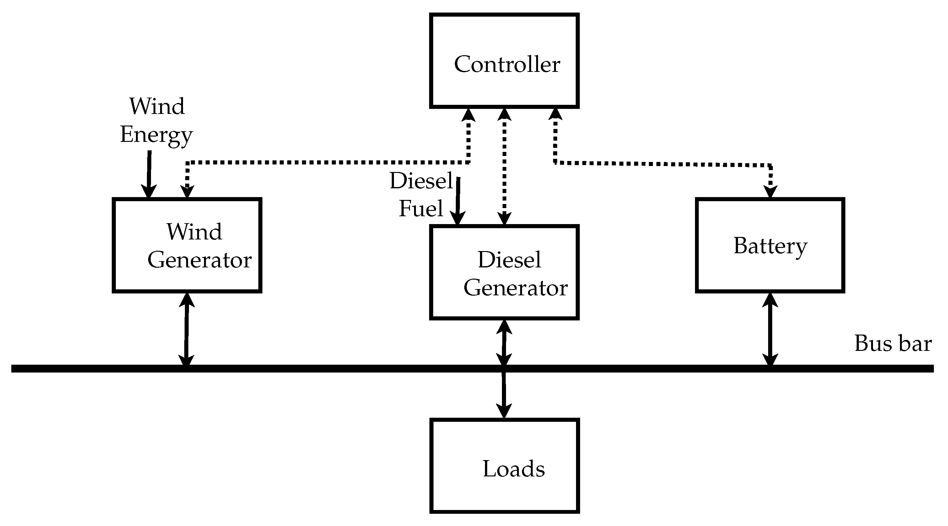
- The hybrid wind–diesel system is described by the linearized model (3).
- The full state vector is available for feedback.
- Plant matrices are controllable/stabilizable.
- The communication network is noiseless and delay-free.
- The event-triggering rule can be continuously verified by the ETC.
6. Robustness of the Developed Event-Triggered Controller
7. Results and Discussion
Robustness Analysis
8. Sensitivity Analysis
9. Conclusions
Author Contributions
Funding
Data Availability Statement
Acknowledgments
Conflicts of Interest
Abbreviations
| ANN | Artificial Neural Network | LQR | Linear Quadratic Regulator |
| ARE | Algebraic Riccati Equation | LTI | Linear Time-invariant |
| ETC | Event-triggered Control | MATI | Maximal Allowable Transmission Interval |
| ETM | Event-triggering Mechanism | NCS | Networked Control Systems |
| HDS | Hybrid Dynamical System | PBH | Popov–Belevitch–Hautus |
| HWDPS | Hybrid Wind–Diesel Power System | SDC | Sampled-data Control |
| LFC | Load Frequency Control | SMC | Sliding Mode Control |
| LMI | Linear Matrix Inequality | ZOH | Zero-Order Hold |
Nomenclature
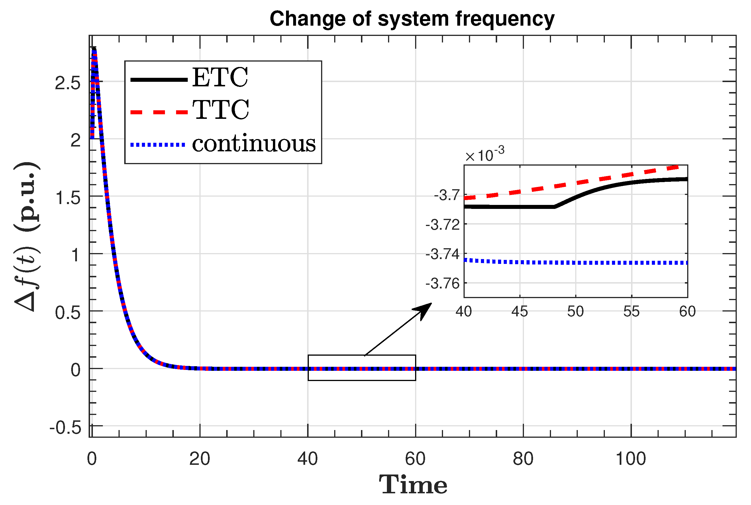
| change in system frequency (puHz) | |
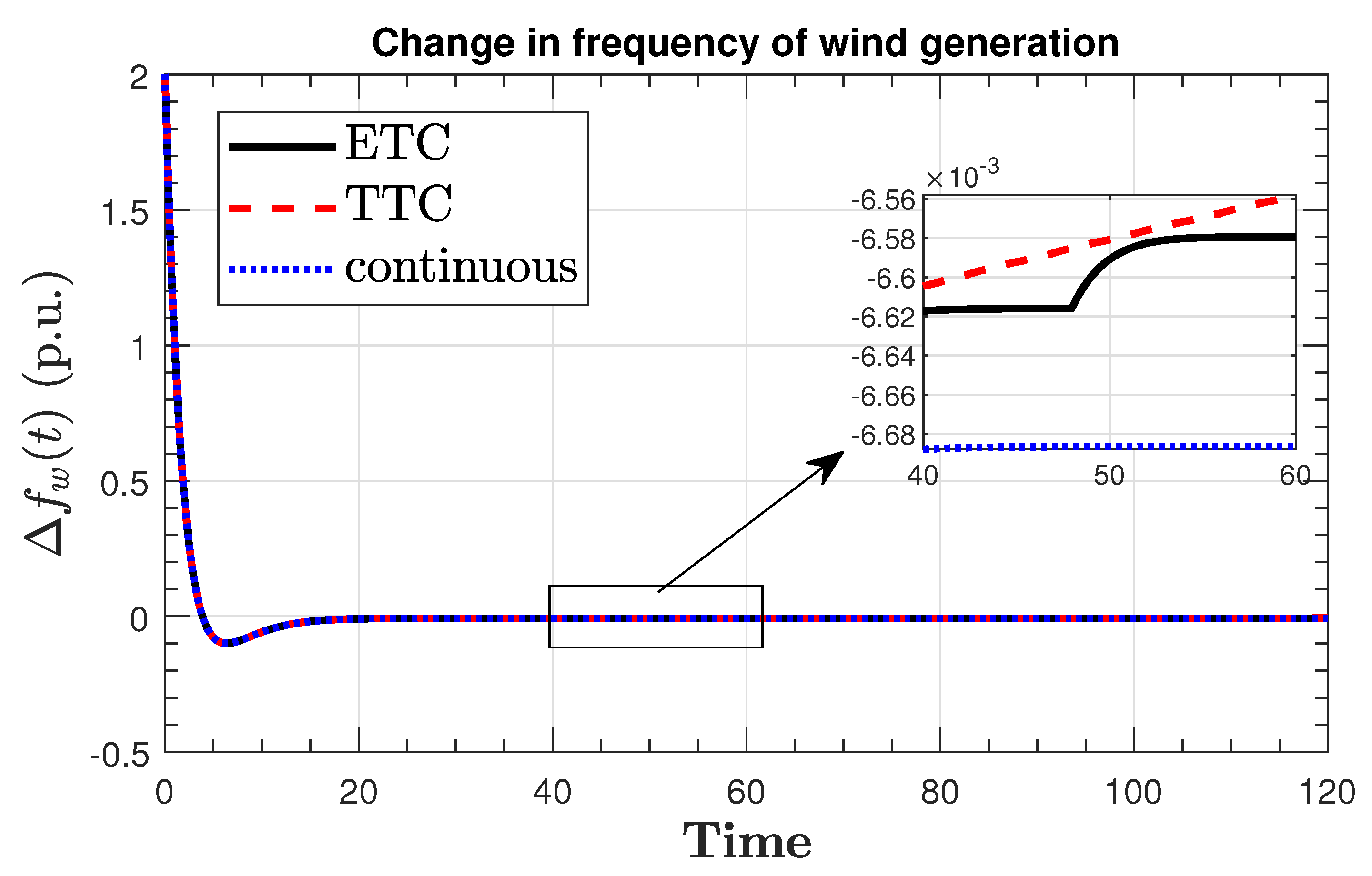
| change in the frequency of wind generation (puHz) | |
| change in the active power of diesel generator (puKW) | |
| change in the active power of wind generation (puKW) | |
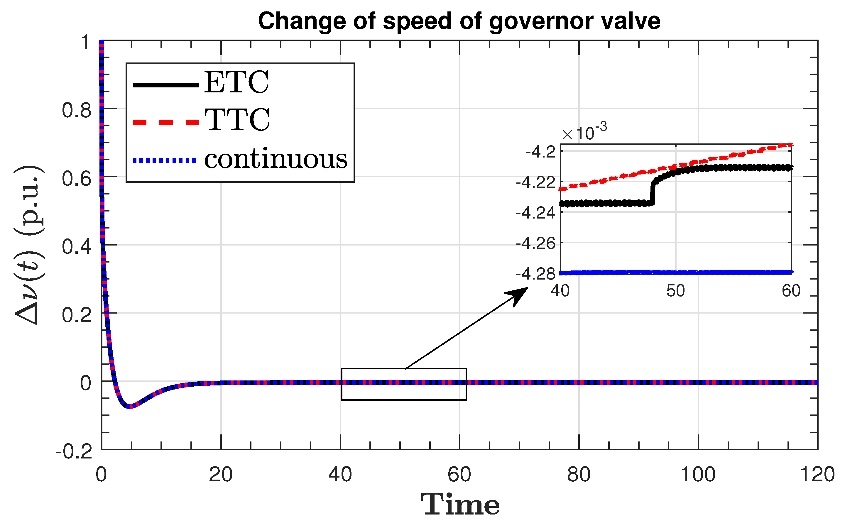
| change in the speed of the governor valve (m/s) | |
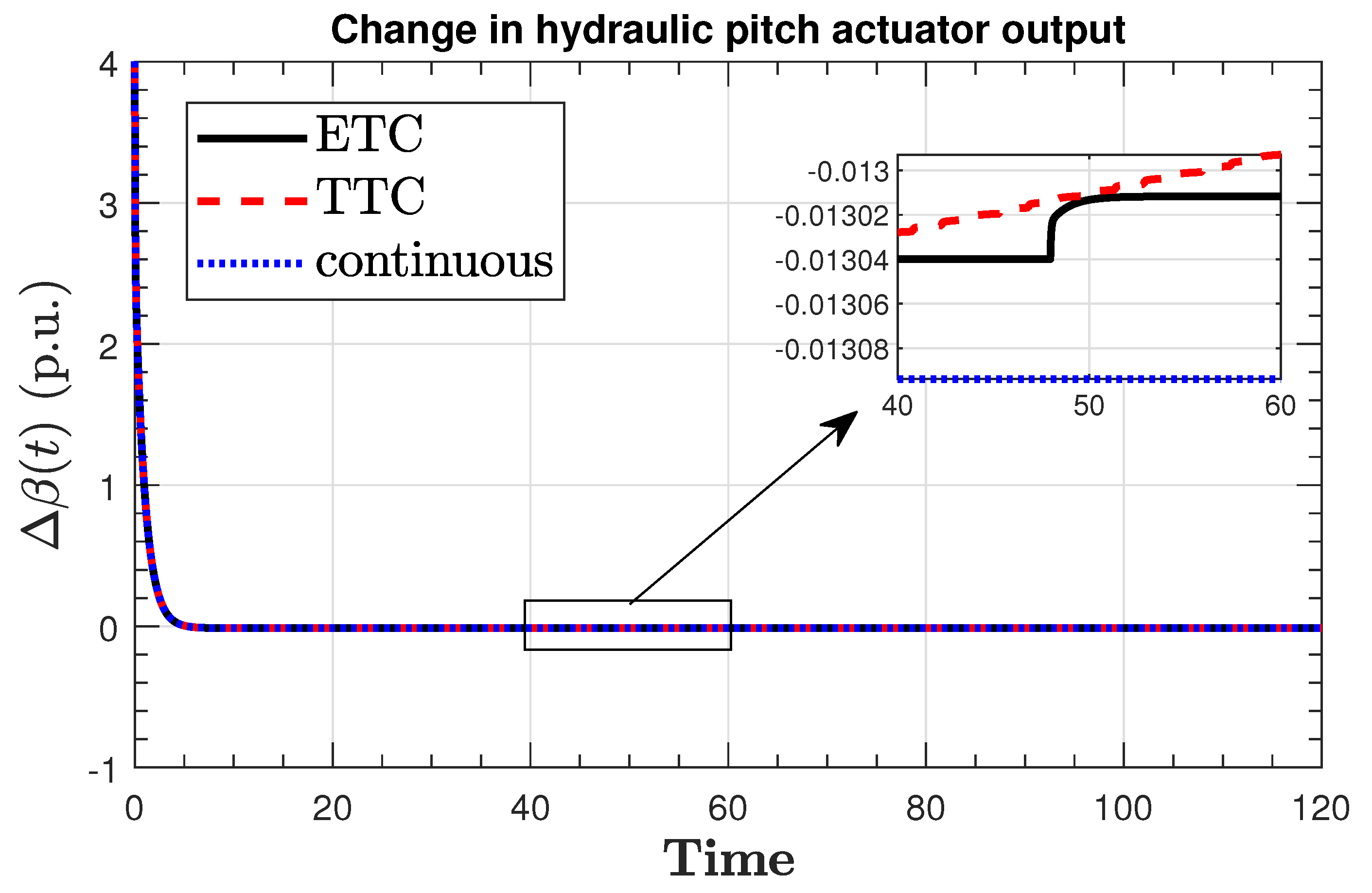
| variation in the output of the hydraulic pitch actuator (puKW) | |
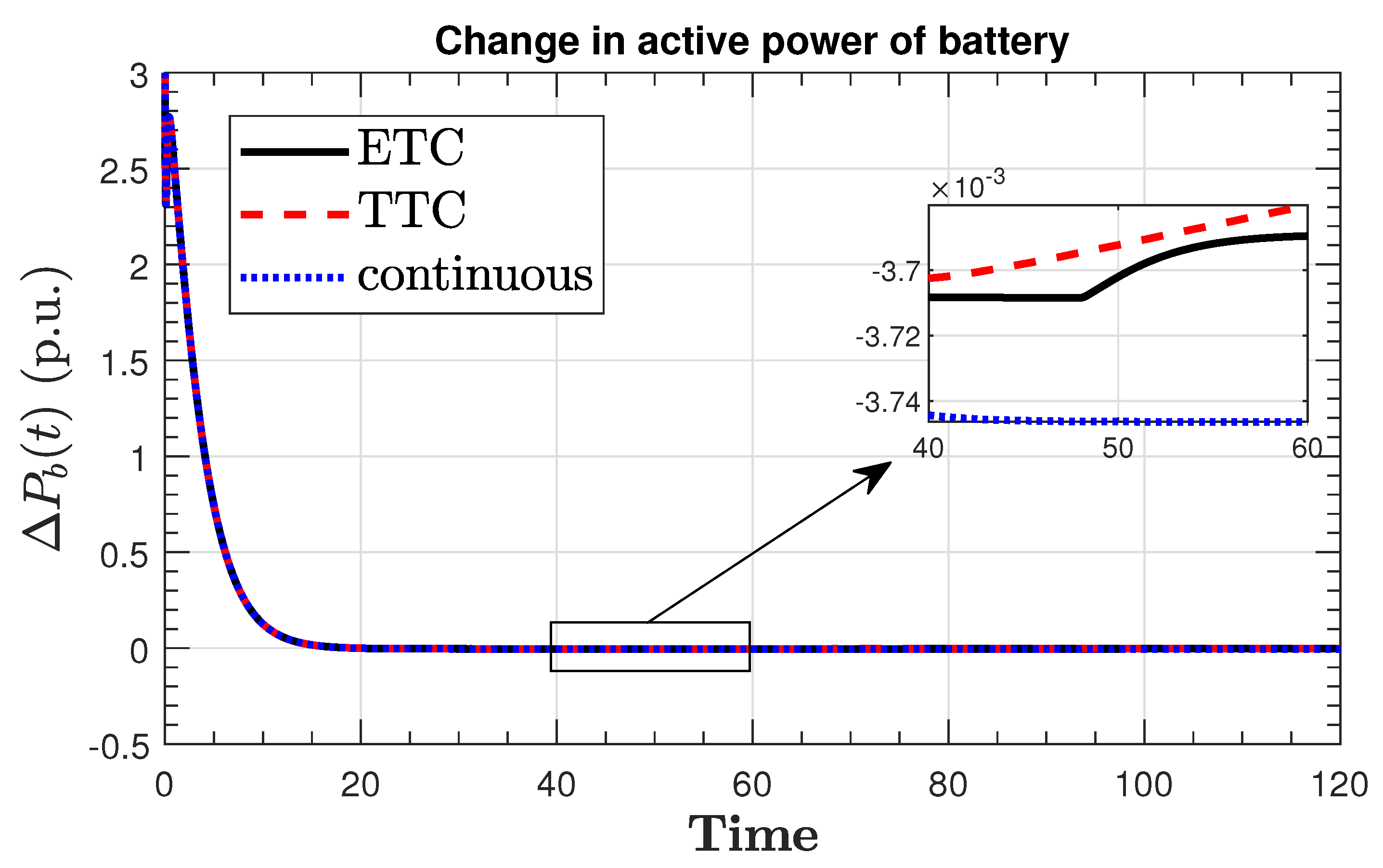
| active power variations of the battery (puKW) |
References
- Shayeghi, H.; Shayanfar, H.; Jalili, A. Load frequency control strategies: A state-of-the-art survey for the researcher. Energy Convers. Manag. 2009, 50, 344–353. [Google Scholar] [CrossRef]
- Shankar, R.; Pradhan, S.; Chatterjee, K.; Mandal, R. A comprehensive state of the art literature survey on LFC mechanism for power system. Renew. Sustain. Energy Rev. 2017, 76, 1185–1207. [Google Scholar] [CrossRef]
- Latif, A.; Hussain, S.; Das, D.; Ustun, T. State-of-the-art of controllers and soft computing techniques for regulated load frequency management of single/multi-area traditional and renewable energy based power systems. Appl. Energy 2020, 266, 114858. [Google Scholar] [CrossRef]
- Hote, Y.; Jain, S. PID controller design for load frequency control: Past, Present and future challenges. IFAC-PapersOnLine 2018, 51, 604–609. [Google Scholar] [CrossRef]
- Sondhi, S.; Hote, Y. Fractional order PID controller for load frequency control. Energy Convers. Manag. 2014, 85, 343–353. [Google Scholar] [CrossRef]
- Alayi, R.; Zishan, F.; Seyednouri, S.; Kumar, R.; Ahmadi, M.; Sharifpur, M. Optimal Load Frequency Control of Island Microgrids via a PID Controller in the Presence of Wind Turbine and PV. Sustainability 2021, 13, 10728. [Google Scholar] [CrossRef]
- Jamii, J.; Mansouri, M.; Trabelsi, M.; Mimouni, M.; Shatanawi, W. Effective artificial neural network-based wind power generation and load demand forecasting for optimum energy management. Front. Energy Res. 2022, 10, 898413. [Google Scholar] [CrossRef]
- Dhibi, K.; Mansouri, M.; Trabelsi, M.; Abodayeh, K.; Bouzrara, K.; Nounou, H.; Nounou, M. Enhanced PSO-Based NN for Failures Detection in Uncertain Wind Energy Systems. IEEE Access 2023, 11, 15763–15771. [Google Scholar] [CrossRef]
- Dokht Shakibjoo, A.; Moradzadeh, M.; Moussavi, S.; Mohammadzadeh, A.; Vandevelde, L. Load frequency control for multi-area power systems: A new type-2 fuzzy approach based on Levenberg–Marquardt algorithm. ISA Trans. 2022, 121, 40–52. [Google Scholar] [CrossRef]
- Khadanga, R.; Kumar, A.; Panda, S. Frequency control in hybrid distributed power systems via type-2 fuzzy PID controller. IET Renew. Power Gener. 2021, 15, 1706–1723. [Google Scholar] [CrossRef]
- Muthukumari, S.; Kanagalakshmi, S.; Sunil Kumar, T.K. Optimal Tuning of LQR for Load Frequency Control in Deregulated Power System for Given Time Domain Specifications. In Proceedings of the 2019 29th Australasian Universities Power Engineering Conference (AUPEC), Nadi, Fiji, 26–29 November 2019; pp. 1–6. [Google Scholar] [CrossRef]
- Ali, T.; Malik, S.A.; Hameed, I.; Daraz, A.; Mujlid, H.; Azar, A. Load Frequency Control and Automatic Voltage Regulation in a Multi-Area Interconnected Power System Using Nature-Inspired Computation-Based Control Methodology. Sustainability 2022, 14, 12162. [Google Scholar] [CrossRef]
- Liu, J.; Yao, Q.; Hu, Y. Model predictive control for load frequency of hybrid power system with wind power and thermal power. Energy 2019, 172, 555–565. [Google Scholar] [CrossRef]
- Daraz, A.; Malik, S.; Azar, A.; Aslam, S.; Alkhalifah, T.; Alturise, F. Optimized Fractional Order Integral-Tilt Derivative Controller for Frequency Regulation of Interconnected Diverse Renewable Energy Resources. IEEE Access 2022, 10, 43514–43527. [Google Scholar] [CrossRef]
- Li, C.; Wu, Y.; Sun, Y.; Zhang, H.; Liu, Y.; Liu, Y.; Terzija, V. Continuous Under-Frequency Load Shedding Scheme for Power System Adaptive Frequency Control. IEEE Trans. Power Syst. 2020, 35, 950–961. [Google Scholar] [CrossRef]
- Horri, R.; Mahdinia Roudsari, H. Adaptive Under-Frequency Load-Shedding Considering Load Dynamics and Post Corrective Actions to Prevent Voltage Instability. Electr. Power Syst. Res. 2020, 185, 106366. [Google Scholar] [CrossRef]
- Dahab, Y.; Abubakr, H.; Mohamed, T. Adaptive Load Frequency Control of Power Systems Using Electro-Search Optimization Supported by the Balloon Effect. IEEE Access 2020, 8, 7408–7422. [Google Scholar] [CrossRef]
- Guo, J. Application of a novel adaptive sliding mode control method to the load frequency control. Eur. J. Control 2021, 57, 172–178. [Google Scholar] [CrossRef]
- Prasad, S.; Purwar, S.; Kishor, N. Load frequency regulation using observer based non-linear sliding mode control. Int. J. Electr. Power Energy Syst. 2019, 104, 178–193. [Google Scholar] [CrossRef]
- Mi, Y.; Song, Y.; Fu, Y.; Wang, C. The Adaptive Sliding Mode Reactive Power Control Strategy for Wind–Diesel Power System Based on Sliding Mode Observer. IEEE Trans. Sustain. Energy 2020, 11, 2241–2251. [Google Scholar] [CrossRef]
- Karafyllis, I.; Kravaris, C. From continuous-time design to sampled-data design of observers. IEEE Trans. Autom. Control 2009, 59, 2169–2174. [Google Scholar] [CrossRef]
- Chen, T.; Francis, B. Optimal Sampled-Data Control Systems; Springer Inc.: New York, NY, USA, 1995. [Google Scholar]
- Nešić, D.; Teel, A.; Carnevale, D. Explicit Computation of the Sampling Period in Emulation of Controllers for Nonlinear Sampled-Data Systems. IEEE Trans. Autom. Control 2009, 54, 619–624. [Google Scholar] [CrossRef]
- Carnevale, D.; Teel, A.; Nešić, D. A Lyapunov proof of an improved maximum allowable transfer interval for networked control systems. IEEE Trans. Autom. Control 2007, 52, 892–897. [Google Scholar] [CrossRef]
- Zhang, X.M.; Han, Q.L.; Ge, X.; Ning, B.; Zhang, B.L. Sampled-data control systems with non-uniform sampling: A survey of methods and trends. Annu. Rev. Control 2023, 55, 70–91. [Google Scholar] [CrossRef]
- Abdelrahim, M.; Postoyan, R.; Daafouz, J. Event-triggered control of nonlinear singularly perturbed systems based only on the slow dynamics. In Proceedings of the IFAC Symposium on Nonlinear Control systems, Toulouse, France, 4–6 September 2013; pp. 347–352. [Google Scholar] [CrossRef]
- Borgers, D.; Heemels, W. Event-Separation Properties of Event-Triggered Control Systems. IEEE Trans. Autom. Control 2014, 59, 2644–2656. [Google Scholar] [CrossRef]
- Abdelrahim, M.; Dolk, V.; Heemels, W. Input-to-state stabilizing event-triggered control for linear systems with output quantization. In Proceedings of the 55th IEEE Conference on Decision and Control, Las Vegas, NV, USA, 12–14 December 2016; pp. 483–488. [Google Scholar] [CrossRef]
- Soltaninejad, M.; Ghiasi, A.R.; Ghaemi, S.; Bagheri, P. Quantized event-triggered H∞ control of linear networked systems with time-varying delays and packet losses. Optim. Control. Appl. Methods 2020, 41, 327–348. [Google Scholar] [CrossRef]
- Aranda-Escolástico, E.; Abdelrahim, M.; Guinaldo, M.; Dormido, S.; Heemels, W. Design of periodic event-triggered control for polynomial systems: A delay system approach. IFAC-PapersOnLine 2017, 50, 7887–7892. [Google Scholar] [CrossRef]
- Yan, S.; Gu, Z.; Park, H.J. Memory-Event-Triggered H∞ Load Frequency Control of Multi-Area Power Systems With Cyber-Attacks and Communication Delays. IEEE Trans. Netw. Sci. Eng. 2021, 8, 1571–1583. [Google Scholar] [CrossRef]
- Yan, S.; Gu, Z.; Park, J.H.; Xie, X. Adaptive Memory-Event-Triggered Static Output Control of T–S Fuzzy Wind Turbine Systems. IEEE Trans. Fuzzy Syst. 2022, 30, 3894–3904. [Google Scholar] [CrossRef]
- Lv, M.; Sun, Y.; Wang, Y.; Dinavahi, V. Adaptive Event-Triggered Load Frequency Control of Multi-Area Power Systems Under Networked Environment via Sliding Mode Control. IEEE Access 2020, 8, 86585–86594. [Google Scholar] [CrossRef]
- Xu, K.; Niu, Y.; Yang, Y. Load frequency control for wind-integrated multi-area power systems: An area-based event-triggered sliding mode scheme. J. Frankl. Inst. 2022, 359, 9451–9472. [Google Scholar] [CrossRef]
- Liu, J.; Gu, Y.; Zha, L.; Liu, Y.; Cao, J. Event-Triggered H∞ Load Frequency Control for Multiarea Power Systems Under Hybrid Cyber Attacks. IEEE Trans. Syst. Man Cybern. Syst. 2019, 49, 1665–1678. [Google Scholar] [CrossRef]
- Li, H.; Wang, X.; Xiao, J. Adaptive Event-Triggered Load Frequency Control for Interconnected Microgrids by Observer-Based Sliding Mode Control. IEEE Access 2019, 7, 68271–68280. [Google Scholar] [CrossRef]
- Zhong, Q.; Yang, J.; Shi, K.; Zhong, S.; Li, Z.; Sotelo, M.A. Event-Triggered H∞ Load Frequency Control for Multi-Area Nonlinear Power Systems Based on Non-Fragile Proportional Integral Control Strategy. IEEE Trans. Intell. Transp. Syst. 2022, 23, 12191–12201. [Google Scholar] [CrossRef]
- Yan, S.; Gu, Z.; Park, J.H.; Xie, X. Sampled Memory-Event-Triggered Fuzzy Load Frequency Control for Wind Power Systems Subject to Outliers and Transmission Delays. IEEE Trans. Cybern. 2023, 53, 4043–4053. [Google Scholar] [CrossRef]
- Anand, S.; Dev, A.; Sarkar, M.K. Load Frequency Control for Power Systems with I/O Time Delays Via Discrete-Time Prediction-Based Event-Triggered Control. In Proceedings of the 2021 IEEE Texas Power and Energy Conference (TPEC), College Station, TX, USA, 5 February 2021; pp. 1–6. [Google Scholar] [CrossRef]
- Goebel, R.; Sanfelice, R.; Teel, A. Hybrid Dynamical Systems: Modeling, Stability, and Robustness; Princeton University Press: Princeton, NJ, USA, 2012. [Google Scholar]
- Selivanov, A.; Fridman, E. Event-Triggered H∞ Control: A Switching Approach. IEEE Trans. Autom. Control 2016, 61, 3221–3226. [Google Scholar] [CrossRef]
- Sadabadi, M.; Peaucelle, D. From static output feedback to structured robust static output feedback: A survey. Annu. Rev. Control 2016, 42, 11–26. [Google Scholar] [CrossRef]
- Dahiya, P.; Mukhija, P.; Saxena, A. Design of sampled data and event-triggered load frequency controller for isolated hybrid power system. Int. J. Electr. Power Energy Syst. 2018, 100, 331–349. [Google Scholar] [CrossRef]
- Heemels, W.; Teel, A.; van de Wouw, N.; Nešić, D. Networked Control Systems with Communication Constraints: Tradeoffs between Transmission Intervals, Delays and Performance. IEEE Trans. Autom. Control 2010, 55, 1781–1796. [Google Scholar] [CrossRef]
- Dolk, V.; Borgers, D.; Heemels, W. Dynamic Event-triggered Control: Tradeoffs Between Transmission Intervals and Performance. In Proceedings of the IEEE Conference on Decision and Control, Los Angeles, CA, USA, 15–17 December 2014; pp. 2764–2769. [Google Scholar]
- Nkosi, N.; Bansal, R.C.; Adefarati, T.; Naidoo, R.M.; Bansal, S.K. A review of small-signal stability analysis of DFIG-based wind power system. Int. J. Model. Simul. 2023, 43, 153–170. [Google Scholar] [CrossRef]
- Fu, A.; Mazo, M., Jr. Decentralized periodic event-triggered control with quantization and asynchronous communication. Automatica 2018, 94, 294–299. [Google Scholar] [CrossRef]
- Heemels, W.; Donkers, M.; Teel, A. Model-based periodic event-triggered control for linear systems. Automatica 2013, 49, 698–711. [Google Scholar] [CrossRef]
- Lofberg, J. YALMIP: A toolbox for modeling and optimization in MATLAB. In Proceedings of the 2004 IEEE International Conference on Robotics and Automation (IEEE Cat. No.04CH37508), New Orleans, LA, USA, 26 April–1 May 2004; pp. 284–289. [Google Scholar] [CrossRef]
- Sanfelice, R.G.; Copp, D.; Nanez, P. A toolbox for simulation of hybrid systems in MATLAB/SIMULINK: Hybrid equations (HyEQ) toolbox (HSCC). In Proceedings of the 16th International Conference on Hybrid Systems: Computation and Control, Philadelphia, PA, USA, 8–11 April 2013; pp. 101–106. [Google Scholar] [CrossRef]


| Result | Guaranteed Min Sampling Time | Number of ETC Transmissions |
|---|---|---|
| [43] | 2 s | 31 |
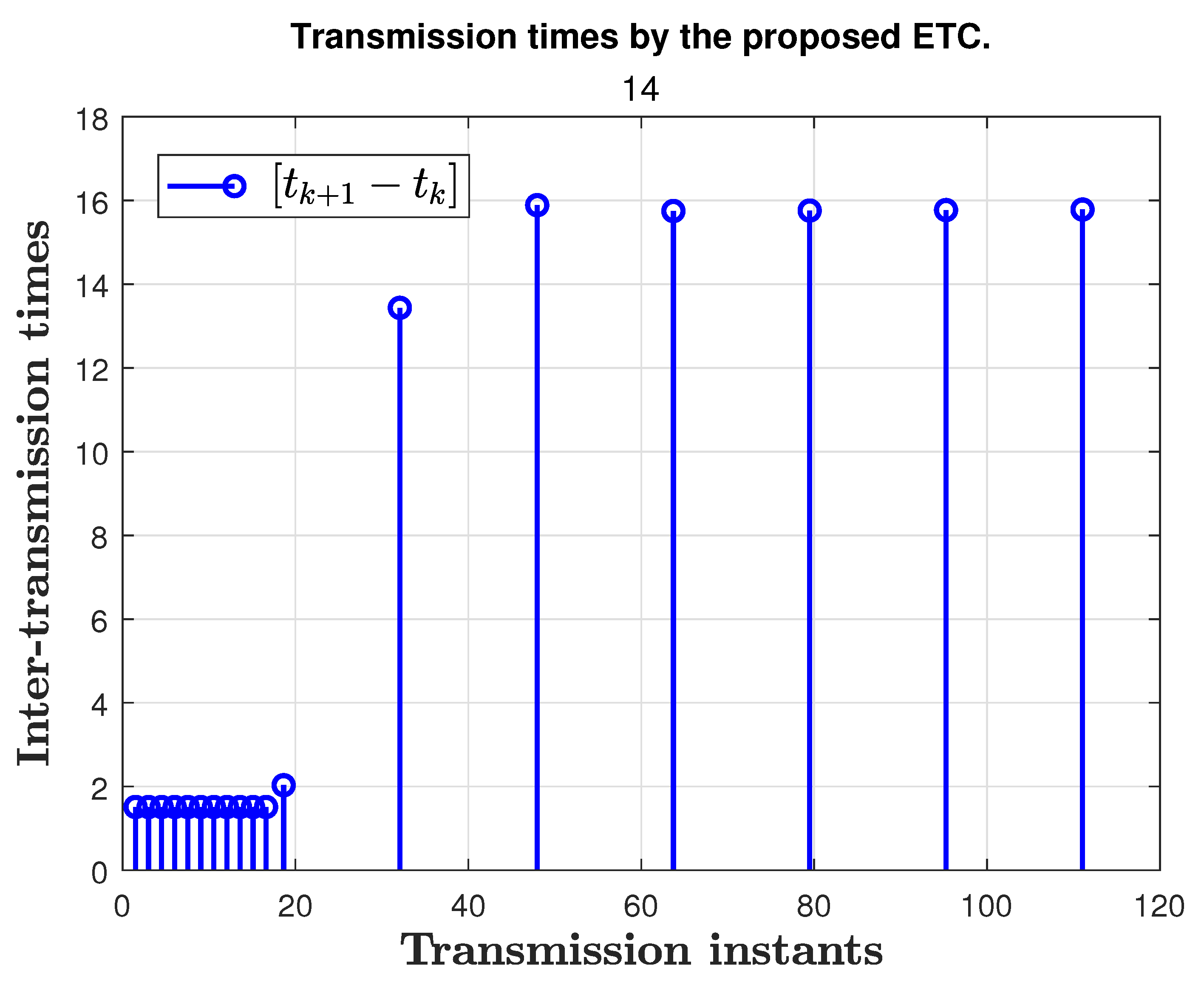
| Proposed ETC technique | s | 18 |
| Result | Periodic Sampling Time | Number of ETC Transmissions |
|---|---|---|
| [43] | 4 s | 21 |
| Proposed ETC technique | s | 18 |
| Parameter | Nominal Value | Min Stabilizing Value | Parameter | Nominal Value | Min Stabilizing Value |
|---|---|---|---|---|---|
Disclaimer/Publisher’s Note: The statements, opinions and data contained in all publications are solely those of the individual author(s) and contributor(s) and not of MDPI and/or the editor(s). MDPI and/or the editor(s) disclaim responsibility for any injury to people or property resulting from any ideas, methods, instructions or products referred to in the content. |
© 2023 by the authors. Licensee MDPI, Basel, Switzerland. This article is an open access article distributed under the terms and conditions of the Creative Commons Attribution (CC BY) license (https://creativecommons.org/licenses/by/4.0/).
Share and Cite
Abdelrahim, M.; Almakhles, D. Synthesis of State/Output Feedback Event-Triggered Controllers for Load Frequency Regulation in Hybrid Wind–Diesel Power Systems. Appl. Sci. 2023, 13, 9652. https://doi.org/10.3390/app13179652
Abdelrahim M, Almakhles D. Synthesis of State/Output Feedback Event-Triggered Controllers for Load Frequency Regulation in Hybrid Wind–Diesel Power Systems. Applied Sciences. 2023; 13(17):9652. https://doi.org/10.3390/app13179652
Chicago/Turabian StyleAbdelrahim, Mahmoud, and Dhafer Almakhles. 2023. "Synthesis of State/Output Feedback Event-Triggered Controllers for Load Frequency Regulation in Hybrid Wind–Diesel Power Systems" Applied Sciences 13, no. 17: 9652. https://doi.org/10.3390/app13179652