A New Method for Evaluating Natural Gas Pipelines Based on ICEEMDAN-LMS: A View of Noise Reduction in Defective Pipelines

Abstract

As the main means of energy transportation, pipelines have the characteristics of 24 h uninterrupted transportation, low cost, strong transmission capacity, and low risk, and they have become an important device for natural gas transportation. However, due to defects caused by the pipeline itself and external forces, it is easy for natural gas leakage to cause major accidents, serious environmental pollution, and huge losses of life and property. Traditional pipeline defect detection technology can be interfered with by a large number of noise signals when collecting defect signals, and the noise reduction method is simple but has poor accuracy, so it cannot directly obtain effective pipeline defect information from the signal and cannot effectively improve the emergency intensity and emergency level of pipeline operation and maintenance management. Therefore, a new noise reduction method, ICEEMDAN-LMS, for natural gas pipelines is proposed in this paper, and the method is calculated and tested in detail. The effectiveness of the new method is verified through the analysis of a pipeline defect signal and normal signal. Moreover, the proposed method can reduce noise more effectively than conventional methods, which has clear value in engineering applications. Importantly, this noise reduction method not only provides a reliable basis for the intelligent diagnosis of pipeline defect signals, but can also be an important reference for helping management departments to make decisions and emergency plans and formulate on-site treatment programs.

1. Introduction

Long-distance pipelines are commonly used in the oil and gas industries. Pipeline defects due to corrosion, natural damage, third-party damage, pipeline materials, and other factors damage the integrity of pipelines, resulting in a reduced service period for each pipeline, and this can even cause a variety of accidents, affecting normal pipeline operation. Therefore, to eliminate the risks to safety and the environment caused by defects, it is necessary to detect these defects using pipeline signals. In the process of pipeline defect detection, when the original defect signal is directly analyzed, high levels of background noise often affect the detection performance and seriously interfere with the final detection result [1]. The detection of pipeline signals is often affected by noise, which reduces the accuracy of pipeline defect diagnosis [2]. Therefore, a precise noise reduction method is needed to suppress noise in pipeline signals and ensure the safe operation of pipelines, which is important in practice. However, the natural gas in a gas pipeline contains impurities and corrosive substances and is affected by external forces, which will continuously wash the pipe body and corrode the pipe wall, resulting in the pipeline pressure distribution being uneven, and pipe wall cracks will appear. When the pipeline has defects, it is easy for natural gas leakage to cause environmental pollution, major accidents, and huge losses of life and property. In order to prevent the occurrence of unsafe pipeline accidents, it is necessary to carry out the comprehensive and accurate detection of pipeline defects. Although existing non-destructive testing technology has many advantages, the pipeline will be disturbed by a lot of noise signals in the process of collecting defect signals. If the pipeline signal is not denoised, effective pipeline defect information cannot be obtained directly from the signal. Therefore, it is necessary to propose an effective signal processing method to reduce the noise of pipeline defect signals, so as to improve the emergency management of pipelines. This is of great significance for the identification, quantification, disaster prevention, and emergency management of pipeline defects [3].

Natural gas pipelines are limited by long laying times, design and operation standards, changes in ground environment facilities, and other factors, and are prone to various defects, leading to pipeline leakage. In order to detect pipeline defects in advance and prevent pipeline disasters, pipeline noise reduction should be carried out before pipeline inspection. However, the traditional pipeline noise reduction method is relatively simple, has poor accuracy, and cannot effectively improve the emergency intensity and emergency level of pipeline operation and maintenance management. However, with the development of science and technology, artificial intelligence is gradually being applied to the noise reduction in natural gas pipelines. For example, deep learning and machine learning methods are applied to the pipeline field to reduce the noise of pipeline signals and assist emergency management departments in making decisions and formulating emergency plans and on-site processing programs [4].

Scholars have carried out a lot of research on noise reduction in the field of transportation [5,6]. Especially in the field of pipeline transportation, scholars have made a lot of contributions to the noise reduction method of pipeline signals. The main traditional noise reduction algorithms are Fourier transform, Wiener filtering, and wavelet transform [7]. Fourier transform is a transform that maps time–domain data to frequency–domain data. Wiener filtering is only suitable for stationary linear signals. Although wavelet transform is suitable for non-stationary signals, it lacks adaptability [8,9]. Many researchers and experts have proposed different approaches to noise reduction. Kalman initially proposed a classification method based on Kalman filters to reduce noise, which improves classification accuracy while preserving defect feature information [10]. However, wavelet filters are superior to Kalman filters in field noise reduction [11]. Wavelet denoising is a time–frequency analysis method that is suitable for non-stationary signal analysis. However, when wavelets are used to analyze pipeline defects, prior knowledge of the signal, appropriate basis function, and decomposition level is required. Moreover, high-frequency noise cannot be completely decomposed, so the reconstructed signal will be distorted. The empirical mode decomposition (EMD) denoising method is a time–frequency analysis method which can decompose complex signals into multiple inherent modal functions based on the signal’s the local characteristic time scale. This method has good adaptive decomposition ability and can handle the denoising of non-stationary and non-linear signals. However, it is prone to modal aliasing during noise reduction [12]. Ensemble empirical mode decomposition (EEMD) obtains the intrinsic mode function (IMF) component by adding white noise, which can alleviate the problem of mode aliasing; however, the process is complex and time-consuming. Therefore, the complete EEMD (CEEMD) method was proposed. In this method, which is based on EMD, different positive and negative noise signals are added to obtain the final IMF component. This method not only compensates for the mode-aliasing problem of EMD, but is also faster than the EEMD method. Moreover, it obtains a more thorough decomposition and reduces noise better. In recent years, scholars have increasingly used EMD to reduce signal noise in different fields such as mechanical vibration, earthquake, and pipeline fault detection [13,14,15]. For example, [14] used the HHT method, which is based on EMD, to study the characteristics of the seismic and explosion waves of natural minerals in coal mines to provide specific guidance for engineering practice. The derivative extremum field mean mode decomposition (DEMMD) method has been employed to study the denoising of pipeline detection signals [16]. However, mode-aliasing and end effects in EMD affect the effectiveness of modal analysis. In addition, EMD is unstable in terms of computation time, and the decomposition performance of multi-frequency signals that consist of similar frequencies is not ideal.

Many theoretical studies have been conducted to address the disadvantages of EMD, mainly focusing on the mode-aliasing problem and construction of the mean curve. For example, [17] proposed using EEMD to add white noise to the original signal to reduce the mode-aliasing problem to a certain extent; however, the amount of calculation was impractical. Moreover, if the original signal has a low signal-to-noise ratio (SNR), residual noise remains in the reconstructed signal. The CEEMD method not only reduces the among of calculation and reconstruction error, but also reduces mode aliasing; however, some problems remain [18]. Using CEEMD, ref. [19] proposed a new fully integrated EMD called CEEMD with adaptive noise (CEEMDAN). The adaptive addition of Gaussian white noise at each stage of the decomposition process enables the method to handle non-stationary and non-linear signals well, yielding an extremely low complete decomposition reconstruction error. Reference [20] proposed the improved CEEMDAN (ICEEMDAN) method, which obtains good denoising accuracy and completeness and can fully compensate for the shortcomings of the above methods.

Although the ICEEMDAN method has many advantages in terms of noise reduction, it only has a significant effect on high-frequency noise signals, and the algorithm performs poorly in the steady state. With regard to signal noise reduction, least mean squares (LMS) not only more comprehensively decomposes the IMF component, but also improves the steady state of the algorithm. As a filter-denoising algorithm based on the steepest gradient descent, the LMS algorithm requires fewer computer resources and is easy to implement. Since its introduction, it has been widely used for signal denoising. Reference [21] proposed an improved LMS algorithm for system noise reduction, which successfully solved the interference problem of complex signal components. The authors of [22] found that the LMS technique has a fast detection speed for signal noise reduction. Reference [23] proposed an improved adaptive algorithm for LMS to perform adaptive filtering and noise reduction processing on fault signals to improve the SNR of the fault signals.

To sum up, the existing traditional noise reduction methods have disadvantages such as mode aliasing, end effect, residual noise, and so on. Therefore, this paper proposes a new hybrid method consisting of ICEEMDAN’s signal decomposition algorithm and IMF’s selection method. This method achieves good denoising accuracy and completeness, which can fully make up for the shortcomings of the above methods. In order to improve the steady-state performance of the noise reduction method, LMS is introduced to improve the steady state of the algorithm. Therefore, ICEEMDAN, combined with the improved LMS method, can not only make the noise reduction more thorough and achieve the ideal noise reduction effect, but also have better robustness.

This study aims to propose a new method to reduce the noise of pipeline defect signals, so as to improve the ability to identify pipeline defects, evaluate the effect of noise reduction, and verify the effectiveness of this method through an example.

The rest of this article is organized as follows. In Section 2, we introduce the basic theory of ICEEMDAN, the LMS, and the basic theory of the improved LMS. Section 3 introduces the ICEEMDAN-LMS method and its noise reduction performance on analog signals. In Section 4, the denoising of pipeline defect signals is evaluated experimentally. Section 5 puts forward the conclusion of this paper and the future research direction.

2. Materials and Methods

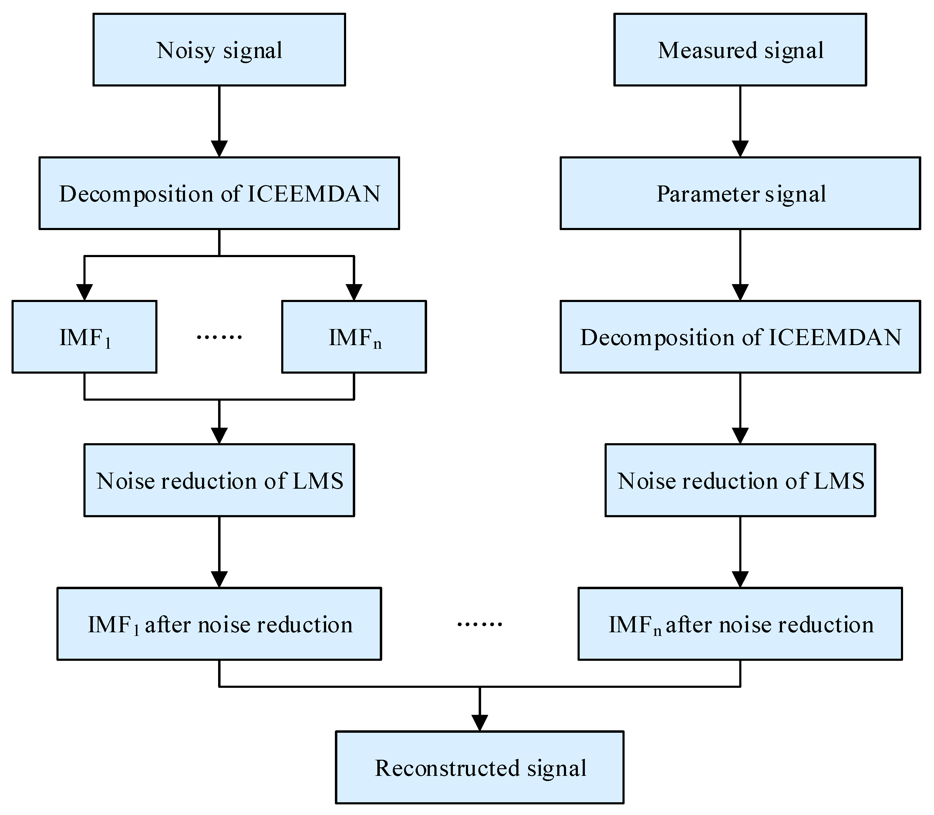
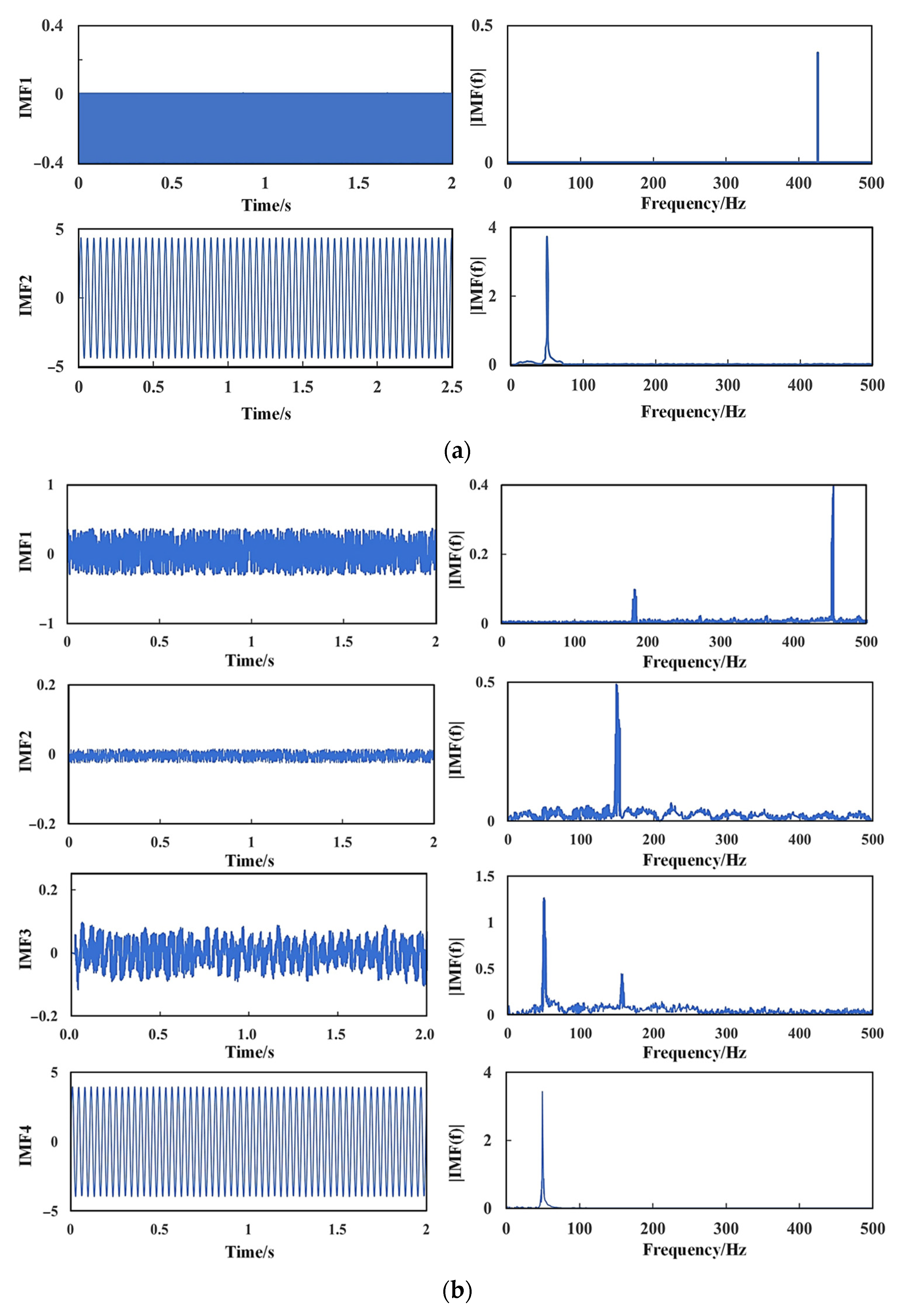
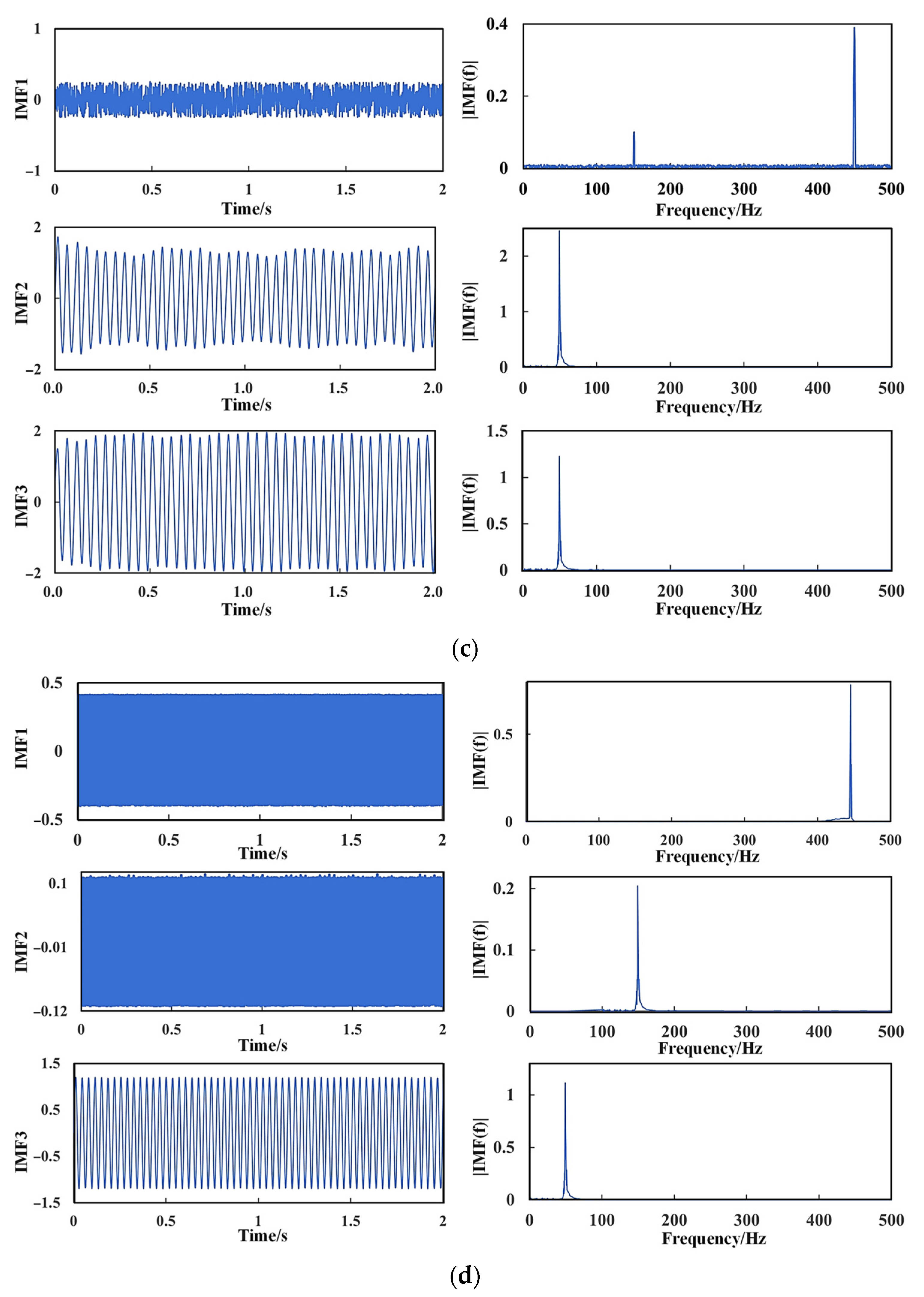
2.1. ICEEMDAN Decomposition Method

EMD can handle the noise reduction in non-linear or non-stationary signals. EMD is based on two basic assumptions:

(a)

For any signal to be analyzed, it can be decomposed into several different basic signal components; whether the component is linear or non-linear, there are equal extreme points and zero crossing points. The component also needs to satisfy the constraint conditions that the local symmetry is 0 and the mean value is 0.

(b)

For a certain point in time, the basic signal components decomposed in the signal to be analyzed can be reconstructed with certain rules to restore the signal to be analyzed. The instantaneous frequency of the signal to be analyzed can be obtained only when all the basic signal components are decomposed. Here, each of the underlying signal components is an intrinsic mode function.

EMD is an adaptive method for the non-stationary signal analysis of non-linear systems but is prone to mode aliasing [24]. To reduce the mode-aliasing phenomenon in EMD, Gaussian noise is added to the entire time–domain space to decompose signals into more regular modes, and this is called EEMD [25]. However, a certain degree of residual noise exists in the EEMD-decomposed eigenmode component, trend component, and reconstructed signal. Complementary EEMD (CEEMD) was proposed to alleviate these problems by adding complementary noise [26]. However, deficiencies still exist in signal integrity and mean decomposition. Therefore, complete EMD with adaptive noise (CEEMDAN), which is based on CEEMD, was proposed and effectively prevents pseudo-modes and residual noise modes [27]; however, some residual noise remains in the decomposed IMF. ICEEMDAN, which is a complete-set EMD with improved adaptive noise, is an improved mode decomposition algorithm based on CEEMDAN that can effectively reduce the generation of pseudo-modal components and solve the residual noise problems existing in the intrinsic modal components, thus increasing the SNR. More precisely, the signal is decomposed into different IMF components, which improves the signal analysis capability [28]. ICEEMDAN’s decomposition process is as follows:

(1)

Add noise ${\eta }^{\mathrm{i}}$ with a mean and variance of 0 and 1, respectively, to the original pipeline signal x to construct a new pipeline signal xⁱ and calculate the local mean of the signal using EMD to obtain a component r_i and several IMF components [29]. Equations (1)–(3) represent the denoted signals, first-order residuals, and first-order IMF components, respectively. The ICEEMDAN method can effectively remove the residual noise and mode aliasing that may exist in the IMF components of the EMD and EEMD algorithms. This is expressed as follows:

$$x^i\left(t\right)=x\left(t\right)+{\beta }_0{E}_1\left({\eta }^i\left(t\right)\right).$$

(1)

$$r_1=〈M\left(x^i\left(t\right)\right)〉.$$

(2)

$$IM{F}_1\left(t\right)=x^i\left(t\right)-r_1\left(t\right).$$

(3)

where $x\left(t\right)$ is a function that describes the value of the signal at different times, and $t$ is the independent variable; ${\eta }^{\mathrm{i}}$ represents Gaussian white noise, where i = 1, 2… n; ${\beta }_0=\frac{{\epsilon }_{0}std\left(x\left(t\right)\right)}{std\left(E_1\left({\eta }^i\left(t\right)\right)\right)}$ represents the noise coefficient; and ${\epsilon }_0$ represents the reciprocal of the expected SNR between the first noise signal and the analyzed signal. Moreover, i represents the number of times noise is added and $std\left(•\right)$ is the standard deviation operator. Finally, $E_k\left(•\right)$ is the k-th mode obtained by EMD, $M\left(•\right)$ represents the local mean value used for the production signal, and $〈•〉$ denotes averaging the whole.

(2)

Add a group of Gaussian white noises to the first-order residual to construct a new signal $r_1\left(t\right)+{\beta }_1{E}_2\left({\eta }^i\left(t\right)\right)$ to be decomposed and obtain the second-order residual $r_2$ and second IMF component using EMD as follows:

$$r_2\left(t\right)=〈M\left(r_1\left(t\right)+{\beta }_1{E}_2\left({\eta }^i\left(t\right)\right)\right)〉.$$

(4)

$$IM{F}_2=r_1\left(t\right)-r_2\left(t\right).$$

(5)

(3)

Similarly, in the k-th order mode, calculate:

$$r_k\left(t\right)=〈M\left(r_{k-1}\left(t\right)+{\beta }_{k-1}{E}_k\left({\eta }^i\left(t\right)\right)\right)〉.$$

(6)

$$IM{F}_k\left(t\right)=r_{k-1}\left(t\right)-r_k\left(t\right).$$

(7)

(4)

Step (3) is repeated until the residual component meets the termination condition or the modal component is less than the local extreme value of the first three orders, and the algorithm outputs all obtained residual and IMF components.

Through the ICEEMDAN process, the characteristic signals at different time scales in the original pipeline signals are decomposed into several IMF components, including the IMF components of the signals indicating the pipeline defects; each modal component is arranged according to frequency. This effectively removes the noise remaining in the intrinsic modal component and greatly reduces the generation of false modal components.

2.2. LMS Method

The LMS algorithm is an adaptive iterative algorithm that was proposed in 1959 by Widrow and Hoff to solve system identification problems [30]. This algorithm cancels out noise from the noisy signal using the reference signal, thereby eliminating the noise in the noisy signal [31]. The objective of the LMS algorithm is to minimize the mean squared error between the known expected response and output signal of the filter, estimate the gradient vector in each iteration according to the input signal, and update the weight coefficient to adapt the algorithm iteratively and output the optimal result. The algorithm has the advantages of a simple structure, high calculation accuracy, easy implementation, and good convergence and stability. Moreover, it has been widely used in many fields to process signals [32]. The expected signal is expressed as follows:

$$E\left[e^2\left(k\right)\right]=E\left({\left[y\left(k\right)-W^T\left(k\right)x\left(k\right)\right]}^2\right).$$

(8)

where $x\left(k\right)$ is the original input noisy signal, $W\left(k\right)$ is the weighted vector of the signal at time k, and $y\left(k\right)$ is the output signal.

Therefore, the filter estimation method based on the LMS algorithm is as follows:

$$w\left(k+1\right)=w\left(k\right)+2\mu e\left(k\right)x\left(k\right).$$

(9)

where $\mu$ is the iteration step size, which has the range $1<\mu <\frac{1}{{\lambda }_{\max }}$, and ${\lambda }_{\max }$ denotes the largest eigenvalue of the autocorrelation matrix.

2.3. Improved LMS Algorithm

Because the step size in conventional LMS is fixed, it cannot achieve both fast convergence and low steady-state misalignment error. The choice of step size $\mu$ in conventional LMS affects the steady-state error as well as the convergence rate of the algorithm; that is, a larger step size increases not only the convergence rate, but also increases the steady-state error and vice versa. In addition, because of the influence of parameter uncertainty, the iteration error and step size of the algorithm are both large during the early iterations, when the convergence speed is high. During the later iterations, the error is always large, resulting in a large step size. Therefore, to address the disadvantages of the LMS algorithm, this study proposes an improved LMS algorithm based on conventional LMS. According to the autocorrelation mean $p\left(k\right)$ of the error signal, the length adjustment parameter $\alpha \left(k\right)$ and waveform size coefficient $\beta \left(k\right)$ are changed. The autocorrelation mean is expressed as follows:

$$p\left(k\right)=mp\left(k-1\right)+N\left(1-m\right)e\left(k\right)e\left(k-1\right).$$

(10)

where $p\left(k\right)$ is the autocorrelation mean of the error signal, N is the interference factor between the error signal and expected signal, and m is the sampling frequency adjustment parameter. Furthermore, we have:

$$\alpha \left(k\right)={\left|\frac{e\left(k\right)}{e\left(k-1\right)}\right|}^2.$$

(11)

$$\beta \left(k\right)=\delta \beta \left(k-1\right)+\gamma p^2\left(k\right).$$

(12)

where $\delta$ and $\gamma$ are fixed constants of the adjustment function.

Then, the step size of the improved LMS is expressed as follows:

$$\mu \left(k\right)=\beta \left(k\right)\left[1-\frac{1}{1+\alpha \left(k\right)\times e^2\left(k\right)}\right].$$

(13)

By adjusting the step size in the improved LMS algorithm, the convergence speed of the weight is accelerated, the algorithm’s steady-state error is reduced, and the performance of the algorithm is improved.

3. Results

3.1. Improved LMS Algorithm

The LMS algorithm is only suitable for single frequencies, and hence, a complex multifrequency signal must be decomposed into a single-frequency signal suitable for LMS processing. ICEEMDAN solves the mode-aliasing problem of the EMD method while reducing the reconstruction error after the CEEMDAN calculation. Complex multi-frequency signals are decomposed into a single IMF component, and noise reduction is then carried out on each IMF component using the adaptive LMS algorithm. That is, the collected original noisy signals are first decomposed into multiple IMF components using ICEEMDAN, and the measured noise signals are also decomposed into multiple IMF components using ICEEMDAN. If the actual noise is difficult to detect, simulated noise can be used instead. After the decomposed multi-scale signals have been obtained, the input signals and noise are decomposed into each frequency band, and then the decomposed components are processed by the improved LMS algorithm to obtain the denoised IMF components. These IMF components are summed to update the signals at different frequency scales. Finally, the denoised signal is reconstructed. Using this signal processing and decomposition, the signal and noise of each frequency band are simplified. Therefore, by adopting this method, the filter-order selection will not be too high, thereby reducing the convergence time and improving the corresponding denoising results. A flowchart of ICEEMDAN-LMS is presented in Figure 1.

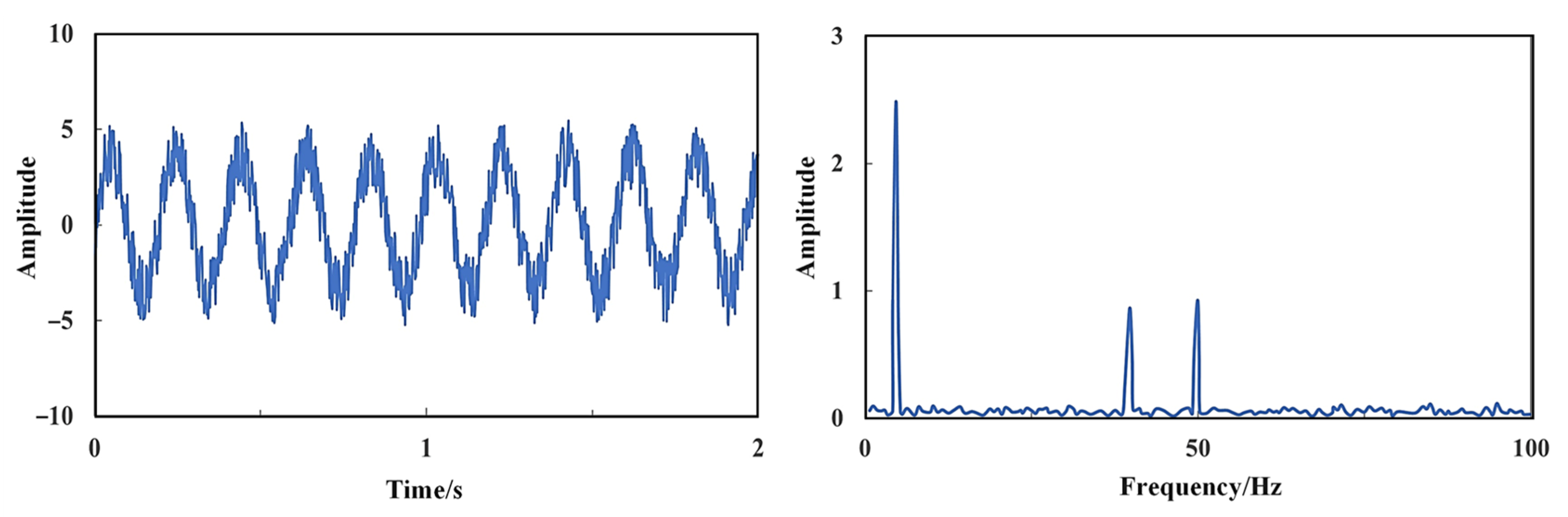
3.2. Pipeline Defect Simulation Signal Analysis

A set of simulation signals comprising normal and noisy signals was designed. In this study, two sinusoidal signals of the same frequency with an amplitude of 2.5 were used, and the result of summing is still the sinusoidal signal of the original frequency. The normal signal is expressed as follows:

$$X=2.5\sin \left(10\pi t\right)+\sin \left(80\pi t\right)$$

Three groups of noise signals were generated as follows:

$${\eta }_1=\sin \left(100\pi t\right)+n\left(t\right)$$

$${\eta }_2=\sin \left(100\pi t\right)+\sin \left(200\pi t\right)+n\left(t\right)$$

$${\eta }_3=\sin \left(100\pi t\right)+\sin \left(200\pi t\right)+\sin \left(1000\pi t\right)+n\left(t\right)$$

where $\eta \left(t\right)$ is Gaussian white noise with a mean of 0 and a variance of 1; $n\left(t\right)$ is Gaussian white noise. To facilitate the calculation, we set the sampling frequency to f_s = 1000 Hz and used N = 1000 sampling points.

Taking the first type of noise as an example, the synthesized signal (denoted as $x_1$) was used for noise reduction. ICEEMDAN was performed on the signals to obtain the corresponding IMF components. Noise ${\eta }_1$ was also decomposed by ICEEMDAN to obtain the corresponding IMF component as a reference signal. Noise signals were filtered by the improved LMS algorithm for each group of IMF components, and the filtered IMF components were summed to obtain the defect signal ${\eta }_{11}$ of the pipeline after noise reduction.

As the time–domain comparison diagrams in Figure 2 and Figure 3 show, the noise of the signal after noise reduction is substantially lower, and the waveform of the signal can be clearly seen. A comparison of the frequency domain diagrams reveals that the main frequency of the pipeline defect signal before noise reduction is concentrated below 100 Hz, and the amplitude of the sinusoidal signal at 100 Hz is reduced from 3.05 to 0.53. In addition, the peak value of the pipeline defect signal is mostly lost in the noise before noise reduction, but the peak value of the effective signal becomes evident after noise removal. As shown in the spectrum diagram of the pipeline defect signal in Figure 3, the visible noise in the spectrum diagram before noise removal is substantially reduced after noise removal. Therefore, when ICEEMDAN is combined with the improved LMS method, it yields a significant reduction in the noise of pipeline defect signals.

As can be seen from

Table 1. Noise removal results.

	s/s11	s/s22	s/s33
SNR/dB	10.66	10.25	9.47
MSE	0.24	0.30	0.38

, ICEEMDAN-LMS obtains good noise reduction results on pipeline defect signals. As the number of superimposed noise signals increases, the root-mean-squared error (RMSE) after noise reduction gradually increases. Adjusting the step size M and order $\mu$ in the LMS algorithm enables ICEEMDAN-LMS to have a significant effect on the data processing of pipeline defect signals when the SNR is greater than −20 dB. However, when the SNR is below −20 dB, the active components of the signal are filtered out. As Figure 4 shows, for added noise over −20 dB, the SNR after denoising increases from −20 dB to −8.5 dB.

After denoising the non-stationary signal of the pipeline defects, it was found that the SNR was improved when the improved LMS method was used (see

Table 2. SNR results for non-stationary signals.

	s/s1	s/s11
SNR/dB	0.09	0.36

).

It can be seen from the above analysis that the ICEEMDAN-LMS method is suitable not only for the noise reduction analysis of stationary pipeline signals, but also for non-stationary signals, and the reduction in noise is substantial. The simulated signal noise reduction results are shown in Figure 5.

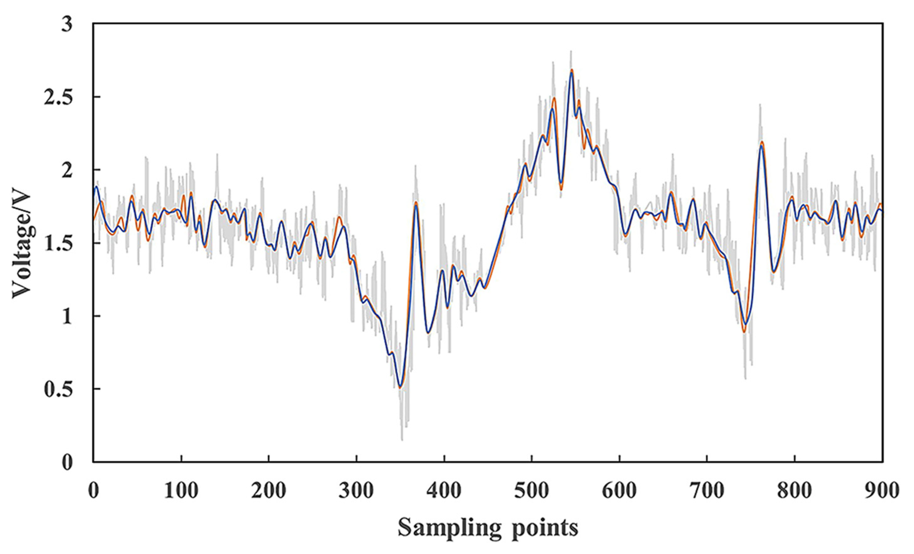
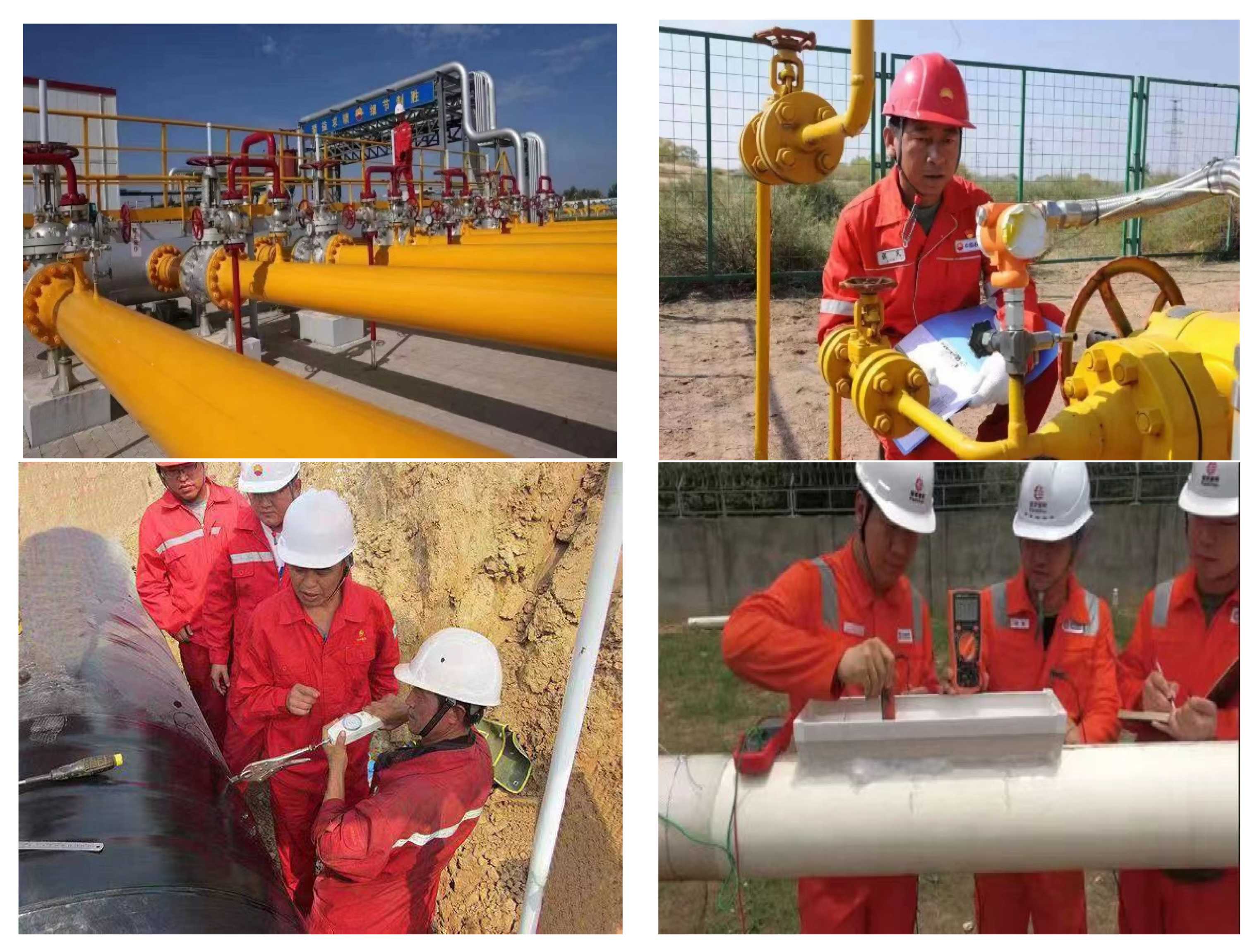
4. Experimental Verification

During gas pipeline defect detection, noise and human interference inevitably exist, which distorts the detection signal and affects the detection. Long-distance pipelines typically pass through complex geological environments. In this study, the magnetic flux leakage detection method was used to detect the pipeline defect signal, and ICEEMDAN-LMS was used to analyze the pipeline defect signal. The reference signals were taken from defect signals measured under normal pipeline working conditions, and the normal signals were filtered to remove high-frequency components. The speed of the detection device of the Shanjing DN250 pipeline was 0.1 m/s, and signals of 14,016 samples in length were obtained in the experiment. The signals were imported into MATLAB for noise removal using ICEEMDAN-LMS. The on-site detection and noise removal results are presented in Figure 6.

ICEEMDAN was used to decompose the signal characteristics of the pipeline signals and compare them with three other EMD-based methods: EEMD, CEEMDAN, and ICEEMDAN [25,33,34]. Figure 7 shows the signal denoising decomposition results of the different methods. As Figure 7a–d show, all four noise reduction methods are suitable for reducing pipeline defect signal noise. Although different methods can eliminate some of the noise, no method performs sufficiently well. Figure 7a shows the decomposition results of the EMD. The original signal has not been completely decomposed, and noise remains in the signal after noise reduction. Moreover, when the signal is highly distorted, the final results are poor. As shown in Figure 7b, the EEMD method is superior to the EMD method in terms of noise reduction; however, the processing of signal distortion remains unsatisfactory, and the mode-aliasing problem still exists in the decomposed eigenmode components. The same problem occurs in the decomposition results of CEEMDAN. As shown in Figure 7c, the denoising performance is better, and progress has been made in the removal of pseudo-modes and residual noise. The results in Figure 7d reveal that the problem of residual noise modes is largely solved, the SNR is increased, and good noise reduction results have been obtained. This method is less effective at suppressing noise and is less robust. Nevertheless, this adaptive denoising method is particularly suitable for denoising pipeline defect signals.

The defect signal is only a part of the pipeline detection results, most of which comprise the detected normal pipeline signal. To evaluate the effectiveness of the proposed denoising method, the EMD, EEMD, CEEMDAN, and ICEEMDAN-LMS methods, which are based on different optimization algorithms, were each used to reduce the noise of field signals. Figure 8 compares the traditional denoising methods and proposed method. First, the signal of a normal pipeline should be denoised; otherwise, the noise signal could be incorrectly identified as the defect signal. Therefore, to evaluate the noise reduction performance for the pipeline defect signal, noise signal, and normal pipeline signal, the SNR and RMSE were used as evaluation criteria:

$$RMSE=\sqrt{\frac{1}{N}{\displaystyle \sum _{t=1}^N{\left[x\left(t\right)-x^{\prime }\left(t\right)\right]}^2}}$$

(14)

$$SNR=10\log \frac{{\displaystyle \sum _{t=1}^N{x}^2\left(t\right)}}{{\displaystyle \sum _{t=1}^N{\left[x\left(t\right)-x^{\prime }\left(t\right)\right]}^2}}$$

(15)

where $x\left(t\right)$ represents the original signal, $x\prime \left(t\right)$ is the denoised signal, and N is the signal length. The RMSE index measures the overall accuracy. The smaller the mean squared error, the better the approximation between the reconstructed and original signals. The SNR is the ratio of the effective signal to the interference signal. The SNR and RMSE were used to evaluate the denoising performance. A larger SNR and smaller RMSE indicate better denoising performance.

To further demonstrate the effectiveness of ICEEMDAN-LMS in reducing pipeline defect signals, ICEEMDAN was first performed on pipeline signals to obtain nine IMF components and residuals. Figure 9 shows the IMF components obtained from the pipeline signal decomposition using EMD and ICEEMDAN. The decomposition of ICEEMDAN is critical because the decomposition results affect the subsequent denoising steps.

According to the decomposition results, the low-frequency components are relatively stable. The fluctuation frequency of each high-frequency component is different, but it also has obvious regularity and small fluctuation in the whole time period. However, the trend of IMF9 generated by EMD is close to the residual component, which indicates that EMD has an over decomposition phenomenon and that the reconstruction error is large. Therefore, ICEEMDAN is more effective in suppressing residual noise and mode-aliasing problems that may exist in the IMF component.

In order to verify the validity of the model proposed in this paper, ICEEMDAN decomposed data were input into the improved LMS model and the noise reduction process of LMS was developed to obtain the noise IMF components and true signal IMF components. In LMS noise reduction, the output of the filter is optimal when the mean squared error is minimized. The optimal output of each frequency band can be combined to reconstruct the denoised signal. The noise reduction results of ICEEMDAN-LMS for pipeline defects are shown in Figure 10 and reveal that the ICEEMDAN-LMS noise reduction method makes the waveform of the pipeline defect signal smoother and more realistic, and most of the high-frequency noise signals have been removed. As presented in

Table 3. Comparison of the SNR and RMSE of the four methods.

Methods	SNR	RMSE
EMD	21.0942	0.0098
EEMD	21.2068	0.0128
CEEMDAN	26.5030	0.0056
ICEEMDAN-LMS	28.4176	0.0039

, ICEEMDAN-LMS yields the highest SNR, indicating that ICEEMDAN-LMS has the largest effective signal proportion and the best noise reduction performance. The minimum mean squared error indicates that the reconstructed and original signals are the most similar. Compared with the CEEMDAN method, ICEEMDAN-LMS improves the SNR by 6.74% and reduces the RMSE by 4.36%. Therefore, ICEEMDAN-LMS improves the SNR and RMSE and hence reduces noise better.

5. Conclusions

In the process of the defect detection of long-distance pipelines, noise interference will inevitably distort the detection signal and affect the detection result. Therefore, the ICEEMDAN-LMS pipeline defect signal denoising method is proposed in this study. The field pipeline defect signal is denoised, and the signal-to-noise ratio and root-mean-squared error are used to evaluate the signal denoising performance.

The contributions of this paper are as follows:

• In this study, by adjusting and improving the step size of LMS, the convergence speed of weights is accelerated and the steady-state error of the algorithm is reduced.
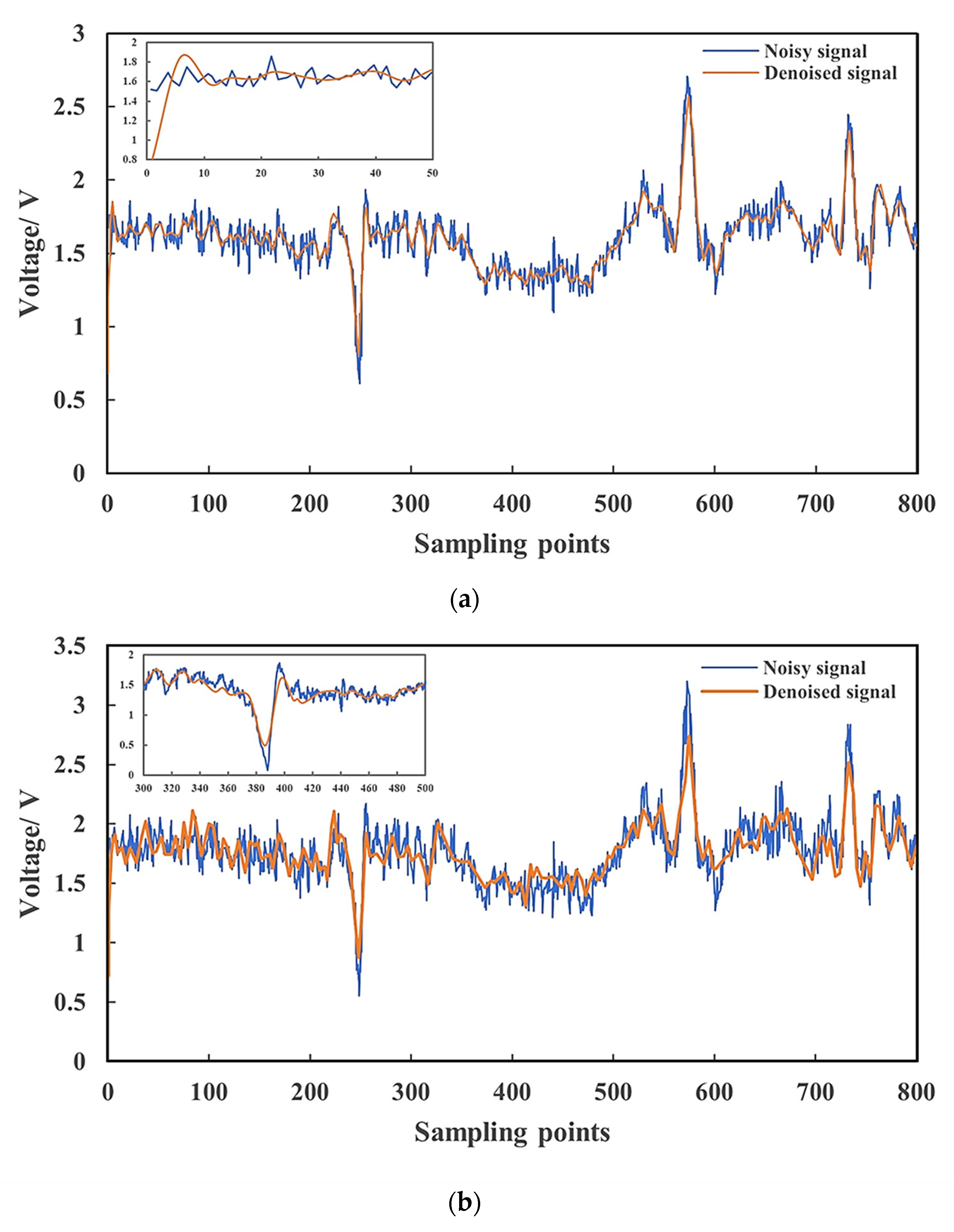
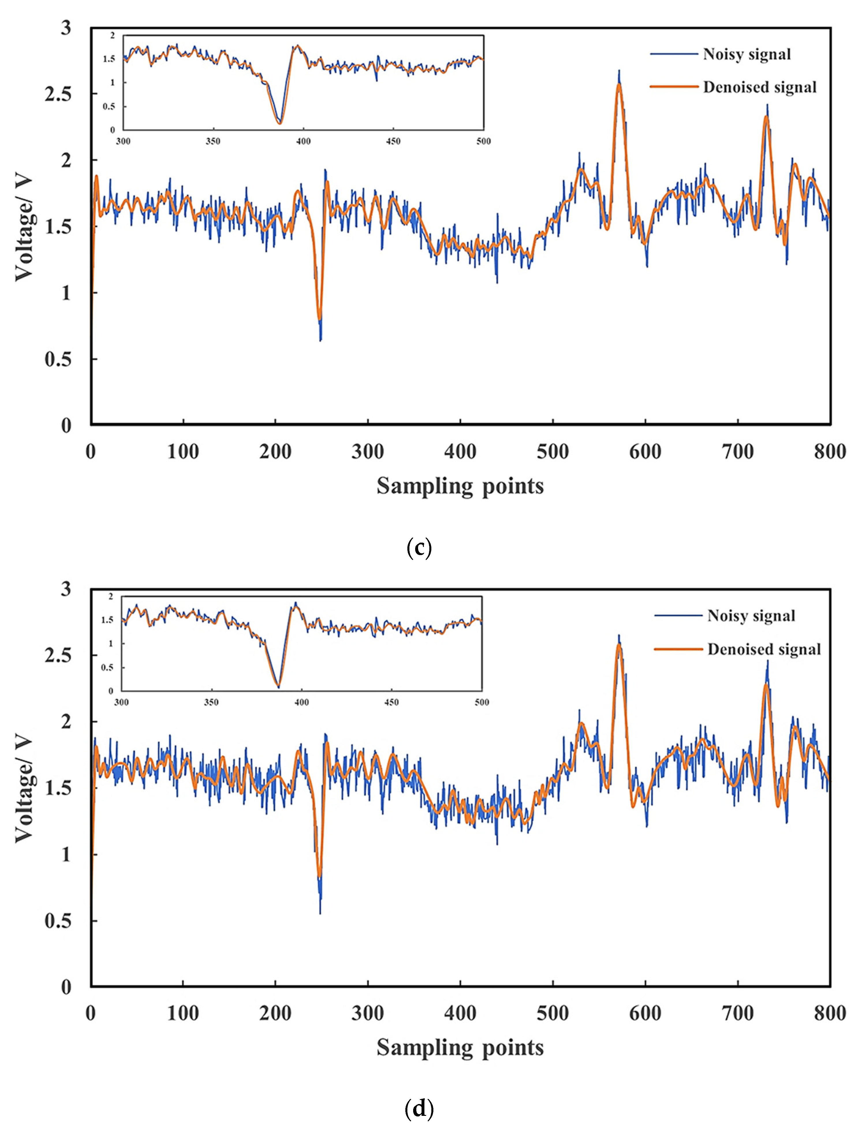
• The superior performance of this method compared with existing methods is verified by simulating pipeline defect signals. The experimental results show that the proposed algorithm can effectively preserve the defect signal and suppress the pipeline noise.
• Compared with the traditional pipeline signal denoising method, the ICEEMDAN-LMS method can improve the signal-to-noise ratio by 6.74% and reduce the root-mean-squared error by 4.36%. The ICEEMDAN-LMS denoising method has the highest signal-to-noise ratio and the lowest RMSE. As a result, ICEEMDAN-LMS improves the signal-to-noise ratio and root-mean-squared error, resulting in a better pipeline noise reduction.

This paper provides a new concept for the noise reduction method and the defect identification of natural gas pipelines and has certain reference value in engineering applications and scientific research experiments. Although this study carried out the field collection and research of defect data and achieved specific results, pipeline leakage caused by pipeline defects is complicated and changeable, and it is necessary to further enrich the signal data of natural gas pipeline defect detection under various circumstances to lay a solid foundation for the realization of big data identification. In addition, how to build a more refined noise reduction model for natural gas pipelines and fully realize the intelligent recognition of pipeline defect signals are challenging tasks. In future studies, the performance of this method will be evaluated from the perspective of the intelligent diagnosis of pipeline defects. We aim to strengthen the emergency analysis and management of long-distance natural gas pipelines and improve the emergency support capacity of natural gas pipeline enterprises.

References

1. Wang, T.X. Characterization of pipeline defect in guided-waves based inspection through matching pursuit with the optimized dictionary. NDT E Int. 2013, 54, 171–182. [Google Scholar]
2. Afzal, M.; Polikar, R.; Udpa, L.; Udpa, S. Adaptive noise cancellation schemes for magnetic flux leakage signals obtained from gas pipeline inspection. Acoust. Speech Signal Proc. 2001, 5, 3389–3392. [Google Scholar]
3. Chen, Y.; Zhang, L.; Hu, J.; Liu, Z.; Xu, K. Emergency response recommendation for long-distance oil and gas pipeline based on an accident case representation model. J. Loss Prev. Process Ind. 2022, 77, 104779. [Google Scholar] [CrossRef]
4. Chen, Y.; Zhang, L.; Hu, J.; Chen, C.; Fan, X.; Li, X. An emergency task recommendation model of long-distance oil and gas pipeline based on knowledge graph convolution network. Process Saf. Environ. Prot. 2022, 167, 651–661. [Google Scholar] [CrossRef]
5. Yan, X.; Wu, Z.; Wang, H. Network noise control under speed limit strategies using an improved bilevel programming model. Transp. Res. Part D Transp. Environ. 2023, 121, 103805. [Google Scholar] [CrossRef]
6. Wang, H.; Zhang, X.; Jiang, S. A Laboratory and Field Universal Estimation Method for Tire–Pavement Interaction Noise (TPIN) Based on 3D Image Technology. Sustainability 2022, 14, 12066. [Google Scholar] [CrossRef]
7. Hammel, S.-M. A noise reduction method for chaotic systems. Phys. Lett. A 1990, 148, 421–428. [Google Scholar] [CrossRef]
8. Almeida, L.-B. The fractional fourier transform and time-frequency representation. IEEE Trans. Signal Process. 1994, 42, 3084–3091. [Google Scholar] [CrossRef]
9. Pratt, W.-K. Generalized wiener filtering computation techniques. IEEE Trans. Comput. 1972, 100, 636–641. [Google Scholar] [CrossRef]
10. Kalman, R.E. A new approach to linear filtering and prediction problems. J. Basic Eng. Trans. ASME 1960, 82, 35–45. [Google Scholar] [CrossRef]
11. Li, F.; Zhang, B.; Verma, S.; Marfurt, K.-J. Seismic signal denoising using thresholded variational mode decomposition. Explor. Geophys. 2017, 49, 450–461. [Google Scholar] [CrossRef]
12. Guo, T.; Deng, Z.-M. An improved EMD method based on the multi-objective optimization and its application to fault feature extraction of rolling bearing. Appl. Acoust. 2017, 127, 46–62. [Google Scholar] [CrossRef]
13. Wang, J.; Du, G.; Zhu, Z.; Shen, C.; He, Q. Fault diagnosis of rotating machines based on the EMD manifold. Mech. Syst. Signal Process. 2020, 135, 106443. [Google Scholar] [CrossRef]
14. Li, X.; Li, Z.; Wang, E.; Feng, J.; Kong, X.; Chen, L.; Li, B.; Li, N. Analysis of natural mineral earthquake and blast based on Hilbert–Huang transform (HHT). J. Appl. Geophys. 2016, 128, 79–86. [Google Scholar] [CrossRef]
15. Lu, W.; Liang, W.; Zhang, L.; Liu, W. A novel noise reduction method applied in negative pressure wave for pipeline leakage localization. Process Saf. Environ. Prot. 2016, 104 Pt A, 142–149. [Google Scholar] [CrossRef]
16. Sha, D.; Liang, W.; Wu, L. A novel noise reduction method for natural gas pipeline defect detection signals. J. Nat. Gas Sci. Eng. 2021, 96, 104335. [Google Scholar] [CrossRef]
17. Wang, T.; Zhang, M.; Yu, Q.; Zhang, H. Comparing the applications of EMD and EEMD on time–frequency analysis of seismic signal. J. Appl. Geophys. 2012, 83, 29–34. [Google Scholar] [CrossRef]
18. Li, J.; Liu, C.; Zeng, Z.; Chen, L. GPR Signal Denoising and Target Extraction with the CEEMD Method. IEEE Geosci. Remote Sens. Lett. 2015, 12, 1615–1619. [Google Scholar]
19. Torres, M.E.; Colominas, M.A.; Schlotthauer, G.; Flandrin, P. A complete ensemble empirical mode decomposition with adaptive noise. In Proceedings of the 2011 IEEE International Conference on Acoustics, Speech and Signal Processing (ICASSP), Prague, Czech Republic, 22–27 May 2011; pp. 4144–4147. [Google Scholar]
20. AL-Musaylh, M.S.; Deo, R.C.; Li, Y.; Adamowski, J.F. Two-phase particle swarm optimized-support vector regression hybrid model integrated with improved empirical mode decomposition with adaptive noise for multiple-horizon electricity demand forecasting. Appl. Energy 2018, 217, 422–439. [Google Scholar] [CrossRef]
21. Ibrahim, G.; Albarbar, A.; Abouhnik, A. Adaptive filtering based system for extracting gearbox condition feature from the measured vibrations. Measurement 2013, 46, 2029–2034. [Google Scholar] [CrossRef]
22. Elasha, F.; Mba, D.; Ruiz-Carcel, C. A comparative study of adaptive filters in detecting a naturally degraded bearing within a gearbox. Mech. Syst. Signal Process. 2016, 3, 1–8. [Google Scholar] [CrossRef]
23. Sahoo, S.; Das, J.-K. Application of adaptive wavelet transform for gear fault diagnosis using modified-LLMS based filtered vibration signal. Recent Adv. Electr. Electron. Eng. 2019, 12, 257–262. [Google Scholar] [CrossRef]
24. Boudraa, A.-O.; Cexus, J.-C. EMD-Based Signal Filtering. IEEE Trans. Instrum. Meas. 2007, 56, 2196–2202. [Google Scholar] [CrossRef]
25. Wu, Z.H.; Huang, N.E. Ensemble empirical mode decomposition: A noise-assisted data analysis method. Adv. Adapt. Data Anal. 2011, 1, 1–41. [Google Scholar] [CrossRef]
26. Yeh, J.-R.; Shieh, J.-S.; Huang, N.-E. Complementary ensemble empirical mode decomposition: A novel noise enhanced data analysis method. Adv. Adapt. Data Anal. 2010, 2, 135–156. [Google Scholar] [CrossRef]
27. Dang, S.; Li, L.; Wang, Q.; Wang, K.; Cheng, P. Fiber optic gyro noise reduction based on hybrid CEEMDAN-LWT method. Measurement 2020, 161, 107865. [Google Scholar]
28. Ali, M.; Prasad, R. Significant wave height forecasting via an extreme learning machine model integrated with improved complete ensemble empirical mode decomposition. Renew. Sustain. Energy Rev. 2019, 104, 281–295. [Google Scholar] [CrossRef]
29. Jiang, Z.; Che, J.; Wang, L. Ultra-short-term wind speed forecasting based on EMD-VAR model and spatial correlation. Energy Convers. Manag. 2021, 250, 114919. [Google Scholar] [CrossRef]
30. Slock, D. On the convergence behavior of the LMS and the normalized LMS algorithms. IEEE Trans. Signal Process. 1993, 41, 2811–2825. [Google Scholar] [CrossRef]
31. Yang, Z.; Huo, L.; Wang, J.; Zhou, J. Denoising low SNR percussion acoustic signal in the marine environment based on the LMS algorithm. Measurement 2022, 202, 111848. [Google Scholar] [CrossRef]
32. Laid, C.; Saad, B. A new pre-whitening transform domain LMS algorithm and its application to speech denoising. Signal Process. 2017, 130, 118–128. [Google Scholar]
33. Luukko, P.-J.-J.; Helske, J.; Räsänen, E. Introducing libeemd: A program package for performing the ensemble empirical mode decomposition. Comput. Stat. 2016, 31, 545–557. [Google Scholar] [CrossRef]
34. Xu, L.; Su, H.; Cai, D.; Zhou, R. RDTS Noise Reduction Method Based on ICEEMDAN-FE-WSTD. IEEE Sens. J. 2022, 22, 17854–17863. [Google Scholar] [CrossRef]
Figure 1. ICEEMDAN-LMS noise reduction process.
Applsci 13 09670 g001
Figure 2. Time–domain and frequency–domain of the pipeline defect signal before noise removal.
Applsci 13 09670 g002
Figure 3. Time–domain and frequency–domain of the pipeline defect signal after noise removal.
Applsci 13 09670 g003
Figure 4. Noise reduction effect when the SNR is −20 dB.
Applsci 13 09670 g004
Figure 5. Simulation signal denoising results.
Applsci 13 09670 g005
Figure 6. Noise reduction diagram of the field detection.
Applsci 13 09670 g006
Figure 7. Decomposition results obtained using (a) EMD, (b) EEMD, (c) CEEMDAN, and (d) ICEEMDAN.
Applsci 13 09670 g007aApplsci 13 09670 g007b
Figure 8. Comparison of traditional and ICEEMDAN-LMS noise reduction methods. (a) EMD, (b) EEMD, (c) CEEMDAN, (d) ICEEMDAN-LMS.
Applsci 13 09670 g008aApplsci 13 09670 g008b
Figure 9. ICEEMDAN denoising decomposition diagram of the pipeline defect signal. (a) EMD (b) ICEEMDAN.
Applsci 13 09670 g009
Figure 10. Test signal noise reduction performance.
Applsci 13 09670 g010