Abstract
The uplifting behaviors of existing tunnels due to overlying excavations are complex and non-linear. They are contributed to by multiple factors, and therefore, they are difficult to be accurately predicted. To address this issue, an extreme gradient boosting (XGBoost) prediction model based on Bayesian optimization (BO), namely, BO-XGBoost, was developed specifically for assessing the tunnel uplift. The modified model incorporated various factors such as an engineering design, soil types, and site construction conditions as input parameters. The performance of the BO-XGBoost model was compared with other models such as support vector machines (SVMs), the classification and regression tree (CART) model, and the extreme gradient boosting (XGBoost) model. In preparation for the model, 170 datasets from a construction site were collected and divided into 70% for training and 30% for testing. The BO-XGBoost model demonstrated a superior predictive performance, providing the most accurate displacement predictions and exhibiting better generalization capabilities. Further analysis revealed that the accuracy of the BO-XGBoost model was primarily influenced by the site’s construction factors. The interpretability of the BO-XGBoost model will provide valuable guidance for geotechnical practitioners in their decision-making processes.
1. Introduction
In recent years, the development of three-dimensional urban transportation has made conducting excavations above existing shield tunnels inevitable [1,2,3,4,5]. During the construction of such excavations, the surrounding soil experiences disturbance, stress release, and uplift at the bottom of the excavation. Consequently, this leads to the force imbalance and uplift of the pre-existing tunnel [6,7].
Numerous studies have been conducted on the deformations of existing tunnels caused by excavations. These studies have primarily employed traditional methods such as theoretical analyses, experimental testing, and numerical simulations [8]. Theoretical analyses based on mechanical principles offer a simpler approach and reveal the underlying laws governing engineering problems [9,10,11,12,13,14,15]. However, these methods often require specific assumptions and consider limited parameters, making them challenging to adapt to different project conditions. Experimental testing, on the other hand, provides intuitive results and can better capture the influences of individual factors [16,17,18,19,20,21,22]. However, it may not fully represent actual project conditions, and the associated costs are generally high. Numerical simulations offer quick and effective means of predicting the impacts of excavations on existing tunnel uplifts. They have been widely applied in the engineering field [23,24,25,26,27]. Nevertheless, the complexities of soils pose challenges in selecting appropriate constitutive models, and the computational capabilities of the software used may impose limitations.
Machine learning models are the outcome of research efforts rooted in statistical theory and optimization algorithms with powerful high-dimensional nonlinear fitting capabilities. The fundamental principle underlying machine learning involves constructing models that learn from extensive datasets to identify patterns and regularities. These trained models can then make predictions for new cases while considering all available information throughout the learning process [28,29].
In the field of underground engineering, various machine learning methods have been applied for prediction purposes, including artificial neural networks (ANNs), random forests (RFs), support vector machines (SVMs), and the extreme gradient boosting (XGBoost) method. Firstly, Shi et al. [30] utilized an ANN method to predict the maximum ground settlement induced by tunnel excavation. Similarly, ANN-based prediction models have been established to intelligently predict soil deformations and geotechnical environmental issues in deep and large excavations and shield tunnel construction projects [31,32,33,34]. Zhou et al. [35] employed an RF algorithm to predict the risk associated with deep excavations in subway stations. Additionally, an auto machine learning (AutoML) -based approach has been proposed for the accurate prediction of tunnel displacements induced by excavations, with successful applications in real-world projects [36]. Researchers have also optimized SVM models to assess horizontal displacements and potential risks during the construction of deep excavations, effectively addressing excavation stability assessment challenges [37,38,39]. Moreover, a multi-step prediction model for rock displacement around tunnels has been proposed based on an SVM model, and its performance has been compared with that of ANN models [40].
Although the aforementioned machine learning methods are effective, they typically consist of single and complex algorithms. Ensemble methods have emerged as superior approaches when compared to individual machine learning methods and other statistical techniques [41,42]. Ensemble methods leverage combining multiple models to achieve higher predictive performances and lower error rates. In the field of shield tunnel construction, Zhou et al. [43] and Su et al. [44] developed XGBoost prediction models using different optimization algorithms. Their research demonstrated that the XGBoost model exhibits notable advantages in terms of accuracy and interpretability, surpassing other models when the prediction results were compared. This highlighted the effectiveness of such ensemble methods, specifically the XGBoost model, in the context of underground engineering applications.
In summary, traditional research methods in the field of geotechnical engineering have often relied on specific assumptions to simplify complex site conditions. However, such a simplified approach has its limitations and can adversely affect the accuracy of research outcomes. In contrast, while machine learning technologies have found widespread applications in predicting foundation deformations and surface settlements, there is a noticeable scarcity of studies focusing on tunnel uplift displacement.
This study introduces an integrated learning algorithm, the BO-XGBoost model, for predicting the uplift displacements of tunnel vaults caused by excavations. The model combines the XGBoost algorithm with a Bayesian optimization (BO) algorithm, optimizing its hyperparameters. A comprehensive database of 170 cases was prepared through extensive engineering research. The data quality and features played a crucial role in determining the upper bound of the model’s accuracy. Therefore, this paper provides a detailed description of the dataset processing. Next, the BO-XGBoost prediction model for tunnel uplift is presented, and its performance is evaluated in comparison to SVM, CART, and unoptimized XGBoost models. The evaluation criteria included root mean square error (RMSE), mean absolute error (MAE), and coefficient of determination (R2) values, which were used to assess the model’s learning and prediction abilities. Furthermore, the interpretability of the BO-XGBoost model is analyzed. The results demonstrate that the BO-XGBoost model exhibited the highest prediction performance for maximum tunnel vault uplift displacements. Moreover, the interpretability of the model will offer valuable guidance to civil engineers during their decision-making processes.
2. Materials and Methods
In order to accurately capture the non-linear impact of multiple factors, it was crucial for the tunnel uplift prediction model to possess strong interpretability. This study addressed this requirement by utilizing an extreme gradient boosting model (XGBoost) as the learning algorithm to establish a prediction model for the maximum uplift displacement of an existing tunnel resulting from excavation. To further enhance the model’s performance, the Bayesian optimization (BO) method was employed to select the optimal hyperparameters for the XGBoost model.
2.1. Algorithm Principle for the XGBoost Model
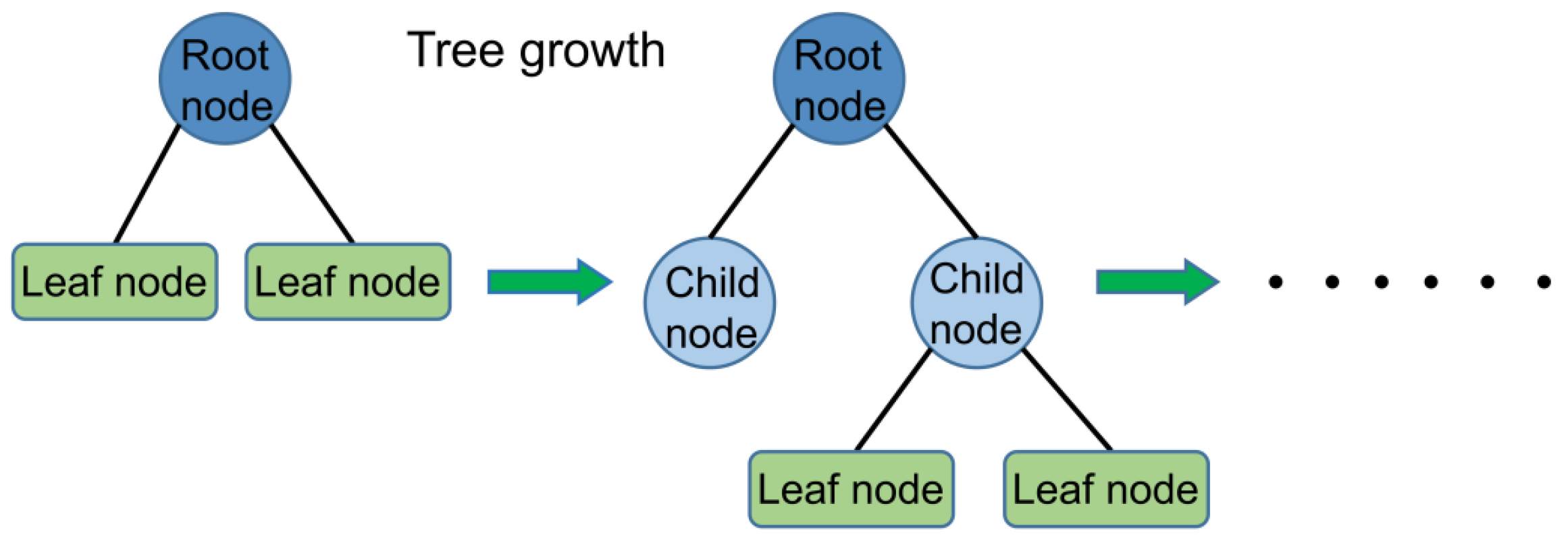
XGBoost, firstly proposed by Washington computer Ph.D. Chen and Guestrin [45], uses CART as a sub-model to achieve the ensemble learning of multiple CART trees by gradient tree boosting. The integration follows the typical additive model and forward distribution algorithm. The basic structure is shown in Figure 1.

Figure 1.
Basic structure of the XGBoost tree model.
The XGBoost algorithm, including the objective function, regularization function, and loss function, enabled it to learn the weights of each feature autonomously with excellent accuracy while being trained. We assumed that the sample dataset used for training was , where , and where is a feature vector with dimensions, denotes the sample label, and the model contains K trees. The XGBoost model was defined as shown in Equation (1):
where is the model prediction value of a sample at the tth iteration, is the model prediction value of sample at the previous iteration, and is the new sub-model trained for the tth time. The objective function (Obj) of the XGBoost model was based on the loss function (L) with the addition of the regularization term (Ω), measuring the complexity of model, as in Equation (2):
The loss function (L) was used for evaluating the deviation between the predicted and measured values of the model. In addition, the regularization term (Ω) was introduced to account for the overall complexity of all trees in the model, effectively mitigating the risk of overfitting [45]. The expression for the regularization term (Ω) is presented in Equation (3):
where γ and λ are both regularization term coefficients, T is the number of leaf nodes in the decision tree, and ω is a vector of the weight scores controlling the leaf nodes. γT affects the complexity of the model by controlling the tree depth.
The optimization objective of the model was to find the optimal loss function satisfying the minimum objective function, and this task was completed by introducing the Taylor formula into the XGBoost model. After expanding Equation (1) using Taylor’s formula and substituting Equation (2) into Equation (1), the objective function was transformed into Equation (4):
During the model training process, a crucial task is to determine the optimal cut points for constructing the tth tree’s leaf nodes. In the XGBoost model, an exact greedy algorithm was adopted to iterate through all the split leaf nodes that were eligible for splitting. Among these nodes, the one with the highest gain in the splitting objective function was chosen as the optimal splitting point. The gain of the splitting point was calculated by Equation (5). Notably, the gain provided a basis for the feature importance output. The steps of the optimal cut-point selection process are outlined in Algorithm 1.
where and denote the first-order gradient statistical sums of the sample sets of the left and right child nodes, respectively, that were split from the current node, and and are the second-order gradient statistical sums of the sample sets of the left and right child nodes, respectively.
| Algorithm 1: Exact Greedy Algorithm for Split Finding |
| Input: I, instance set of the current node, and d, the feature dimension |
for for ) do end end Output: Split with max gain |
2.2. Hyperparameter Optimization Based on Bayesian Algorithm
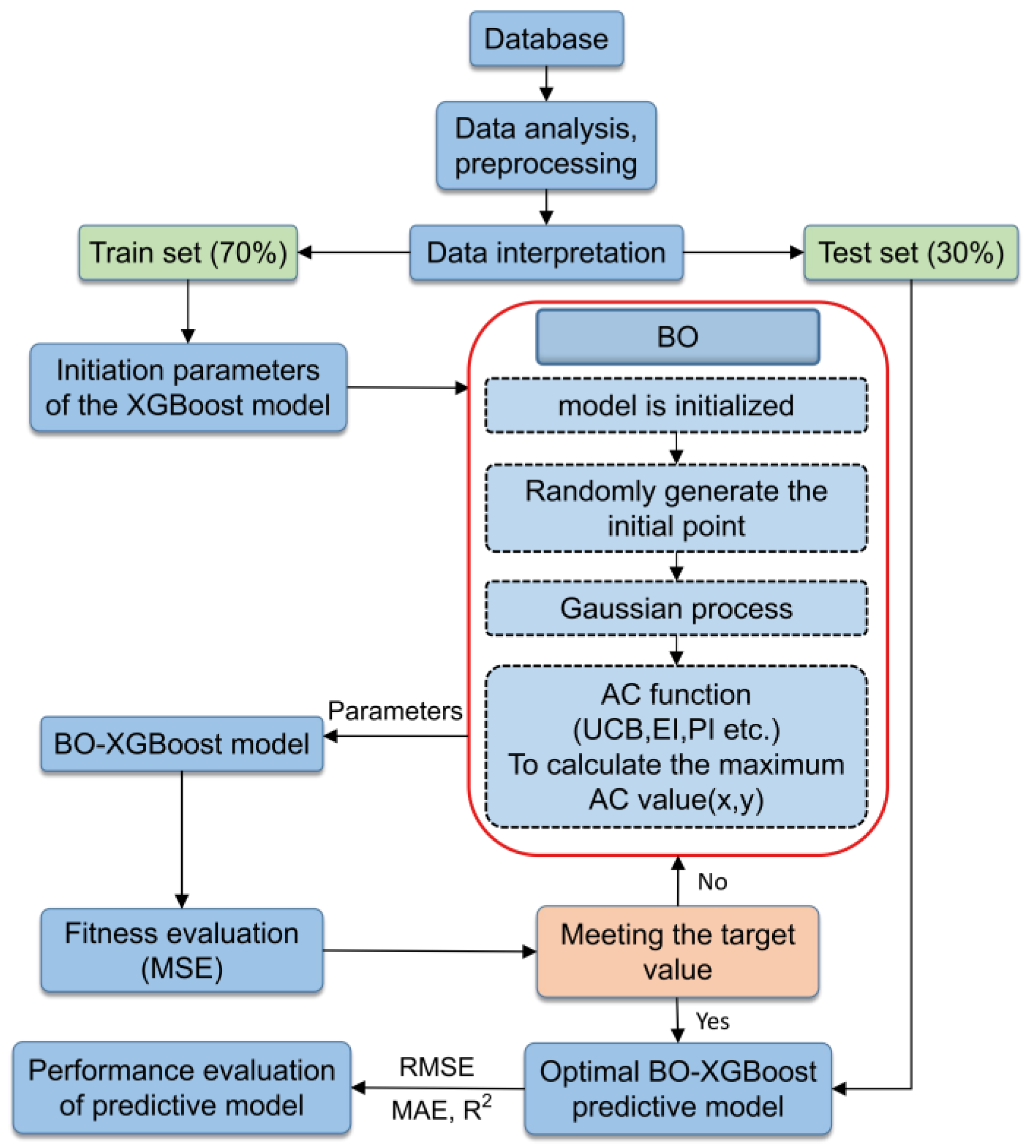
XGBoost, being an integrated tree-based model, inherently possessed a risk of overfitting [43]. To achieve an optimal prediction model performance, it was necessary to conduct hyperparameter optimization prior to training the model. However, such an optimization process can be intricate and time-consuming [46]. Bayesian optimization, on the other hand, leverages information from previous search points to determine the next point to be explored, enhancing both the quality and speed of the search. It is particularly well-suited for fine-tuning parameters with lower dimensionality. The general analysis process of the BO-XGBoost model is illustrated in Figure 2.
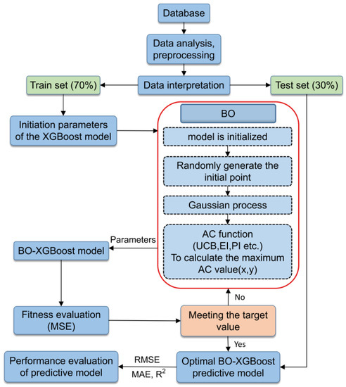
Figure 2.
The overall analysis process of the XGBoost model based on Bayesian optimization.
3. Database-Building and Exploratory Analysis
3.1. Database-Building
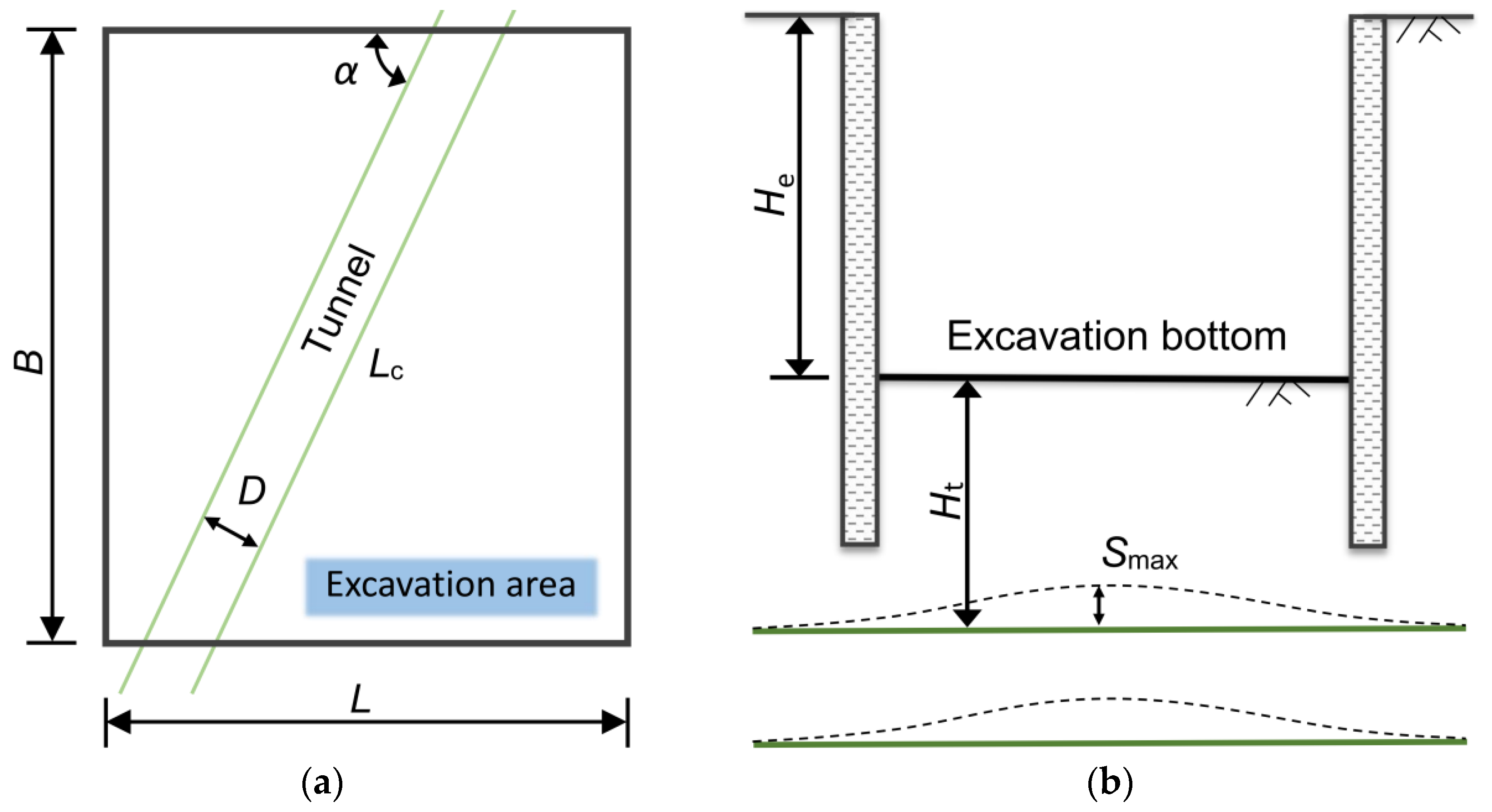
Underground engineering problems are complicated and diverse. In this section, this paper concentrates on the factors influencing the uplift of the underlying tunnel caused by the excavation. Figure 3 shows the relative position between the excavation and the existing tunnel. A database with 170 samples was built by investigating the existing engineering projects, and it was divided into a training set and a test set, with the ratio of 7:3.

Figure 3.
Relative position of the excavation and the tunnel: (a) bird’s eye view, and (b) sectional view.
The relationship between overlying the excavation-induced tunnel uplift and the influencing factors is particularly important for predicting the tunnel uplift. Geological properties are usually essential for determining a construction program. The samples in the database were categorized into four classes according to the properties of the soils in which the existing tunnels were located, namely, muddy silty clay (Mud), soft clay (Sof), silty clay (Sil), and gravelly clay (Gra). The size of an excavation, including its length (L), width (B), and depth (He), directly affects the unloading force exerted on the soil above the tunnel, which, in turn, affects the maximum uplift of the tunnel (Smax). Other factors include the radius of the shield tunnel (D), the distance between the tunnel vault and the base (Ht), and the actual underpass length of the tunnel underpass (Lc). Additionally, the control measures adopted in a project that control the disturbance of the soil by the excavation cannot be overlooked. They are, respectively, the excavation enclosure structure (SWM, DW, and BP), the internal support structure (OC and NC), and other excavation control measures (SM_1, SM_2, SM_3, and SM_4), respectively. It is worth noting that some of these factors are non-numerical variables, such as the soil mixing wall (SWM) in the excavation enclosure structure, which are quantified using binary values (0 and 1), with “1” indicating that the effect of the variable is considered and “0” indicating otherwise. Table 1 presents the definitions, ranges, and detailed descriptions of each variable.

Table 1.
The definitions, ranges, and detailed descriptions of each variable.
3.2. Data Exploratory Analysis
Feature engineering plays a crucial role in determining the quality of a prediction model. Therefore, selecting an optimal subset of features can significantly enhance the accuracy of a model’s predictions. In the initial database, it is common to encounter redundant features. These may include features that exhibit little variation or hold no relevance to the uplift of a tunnel vault, and their included information can be inferred from other features. Removing such redundant features is important for refining the dataset and improving the overall predictive accuracy of a model.
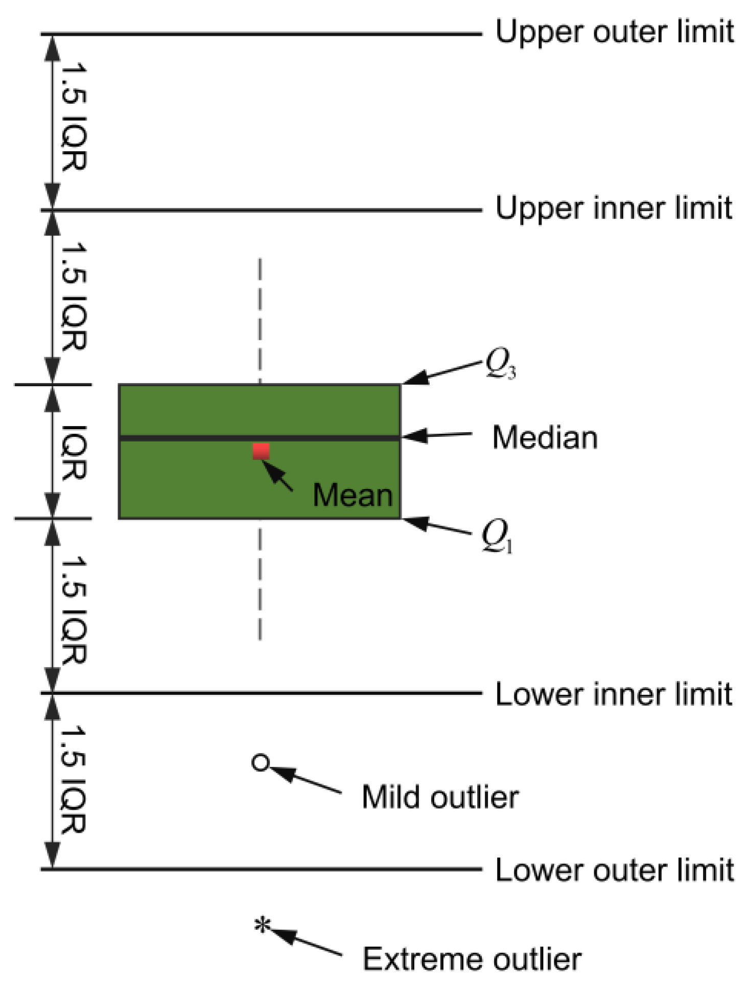
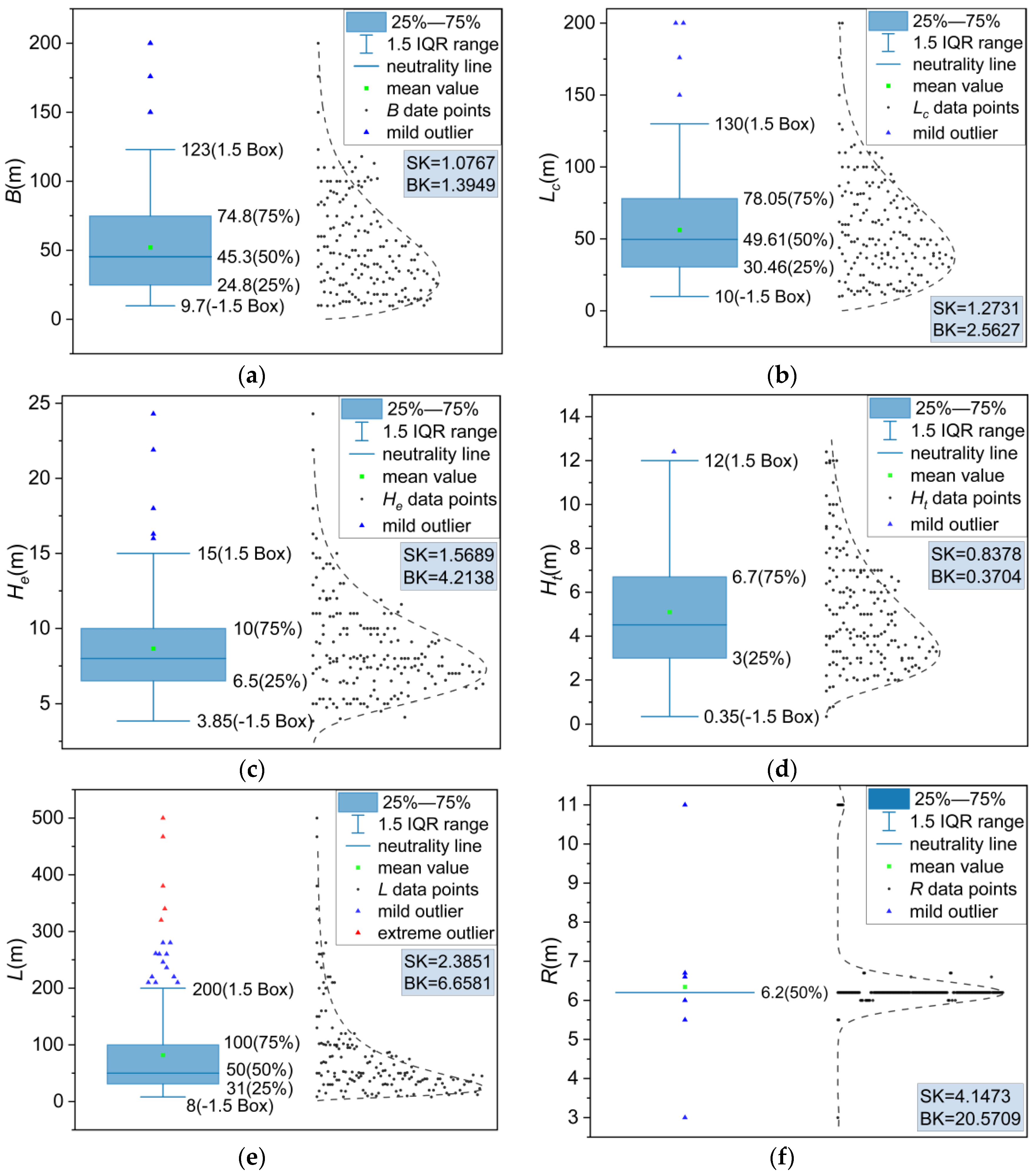
Figure 4 provides an overview of the box plot diagram. The length of the box plot indicates the degree of the data dispersion and the lengths of the upper and lower dashed lines indicate the overall data variances. Considering the soil layers, the samples in the database were categorized into four groups. Figure 5 displays distribution pie chart related to the maximum tunnel uplift (Smax), while Figure 6 illustrates the corresponding box plot. It can be observed that there was a slightly higher proportion of silty clay and soft clay samples, with gravelly clay comprising a smaller portion. This can be attributed to the fact that the engineering cases primarily originated from the southeast coast, such as Shanghai, and these areas experience faster development compared to the central and western regions. Furthermore, Figure 6 shows that the overall sample distribution was relatively even, indicating that the database exhibited good representativeness and universality.

Figure 4.
Box plot diagram.
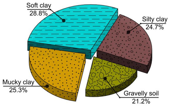
Figure 5.
Soil layer distribution proportion.
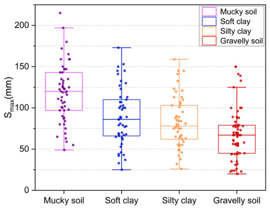
Figure 6.
Smax distribution box plot.
3.2.1. Numeric Variables
To visualize the numerical variables and identify the outliers, a box-normal plot was employed. As shown in Figure 7, the skewness coefficient (SK) and kurtosis (BK) were introduced to depict the distribution patterns of these variables. SK provided information about the direction and extent of skewness in the distribution while BK described the steepness of the distribution pattern.
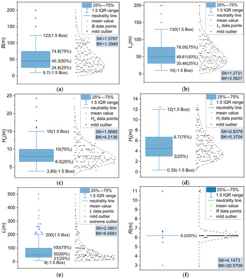
Figure 7.
Numerical variable distribution: (a) B, (b) Lc, (c) He, (d) Ht, (e) L, and (f) R.
As shown in Figure 7f, R had a limited effect on the output Smax, where no significant change was observed. The variables B, Lc, He, and Ht exhibited wider distributions, as shown in Figure 7a–d, and all presented slightly positive skew values (SK > 0). Figure 7e reveals that the variable L was concentrated towards the lower end of the box plot, exhibiting a clear positive skewness. Its kurtosis (BK) was calculated as 6.6581 (after subtracting 3). While some outliers may have held valuable information for training the prediction model, only the extreme outlier of the variable L was removed, as represented by the red triangle in Figure 7e.
The correlation between variables was assessed using Spearman’s correlation coefficient, as illustrated in Figure 8. It could be observed that the variables Lc and B exhibited a high correlation of 0.93 (Lc = B × sinα, where α is the angle of the tunnel passing through the excavation). However, when variables are highly correlated, it can reduce the interpretability of a model. Therefore, in this case, the variable Lc was chosen to train the model with a higher correlation to the output Smax.
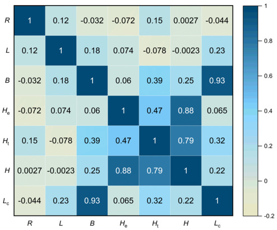
Figure 8.
Correlation matrix.
3.2.2. Categorical Variables
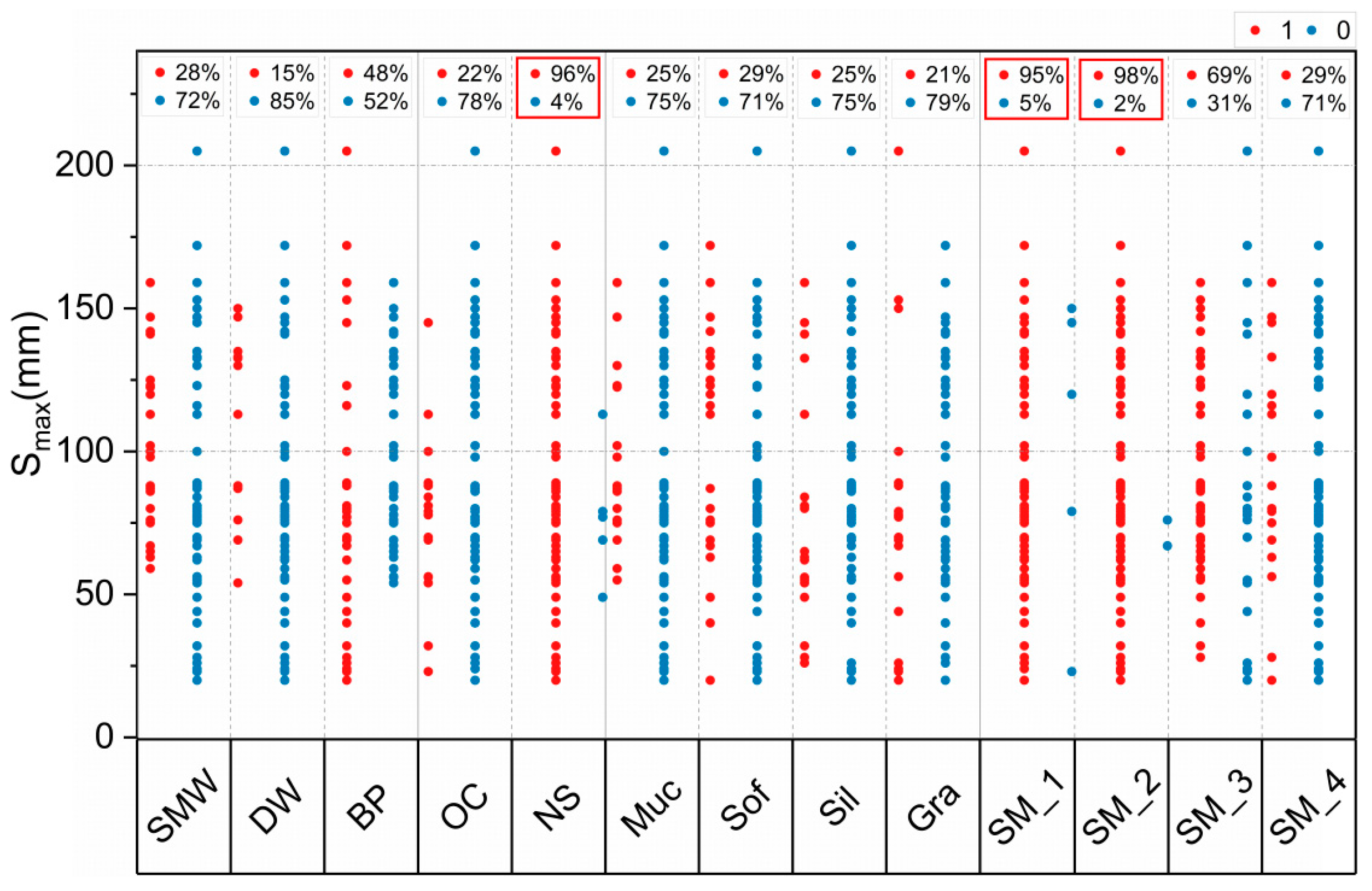
Figure 9 shows a scatter plot of the categorical variables concerning Smax and indicates the variables as percentages of the overall sample size. For instance, the variables SM_1, SM_2, and NS, whose values were concentrated in category “1”, accounted for 95%, 98%, and 96% of the sample size, respectively. This indicated that the construction measures SM_1, SM_2, and NS were used in almost all the cases of the database, thereby making it impossible to identify the effects of these factors on the maximum tunnel uplift. In contrast, the distributions of other categorical variables in relation to Smax exhibited certain patterns, indicating that they played significant guiding roles in the model training process.
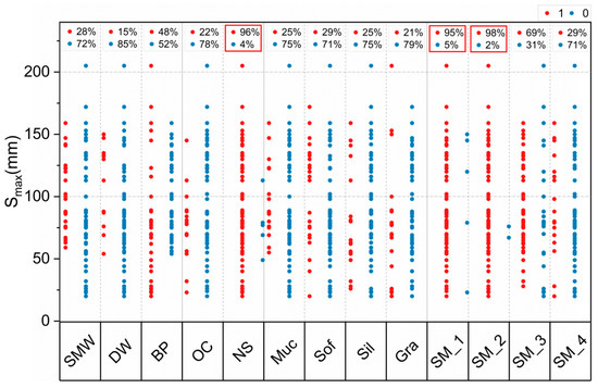
Figure 9.
Categorical variable distribution.
3.3. Data Standardized Processing
To fulfill the computational requirements of models such as SVM and enhance computation efficiency, this study applied Z-score normalization to the data, ensuring a mean value of zero and a standard deviation of one. It was calculated using Equation (6):
where is the mean of all samples and is the standard deviation of all samples. Ultimately, the prediction results of a model are reflected in the original data space.
After processing the sample data using the above methods, the variables B, Lc, He, Ht, SMW, DW, BP, Muc, Sof, Sil, Gra, SM_3, and SM_4 were selected as the inputs of the model, and Smax was the output of the model.
4. Model Prediction Performance Discussion
4.1. Model Creation and Hyperparameter Optimization
As shown in Figure 2, the model-building process included database creation, data processing, database partitioning, model training, result output, and evaluation metrics. The database was derived from engineering cases involving excavations above existing shield tunnels. Before being fed into the model, the data underwent a screening process and were normalized using the Z-score method to mitigate any effects. Of the database, 70% was used as the training set, while the remaining 30% served as the test set.
In this study, the Bayesian optimization method was used to optimize the hyperparameters of the XGBoost model, taking the parameter with the minimum mean square error as the model hyperparameter. To mitigate model overfitting, a five-fold cross-validation iteration was employed. Similar procedures were followed to construct prediction models based on SVM, GBDT, XGBoost, and BO-XGBoost algorithms, and their prediction performances were evaluated using the same dataset. Table 2 provides a summary of the hyperparameters for the XGBoost model, including their descriptions, search scopes, and optimal values.
Table 2.
Search scopes and optimal hyperparameters for each of the XGBoost parameters in the BO tuning process.
Based on the Bayesian search results in Table 2, the optimal XGBoost model hyperparameters were determined to be n_estimators = 43, max_depth = 4, learning_rate = 0.6633, Subsample = 0.9131, Gamma = 14.6795, reg_alpha = 1.5322, and reg_lambda = 16.5579.
4.2. Metrics of the Model Validation and Evaluation
In order to quantitatively evaluate the performances of the training and testing models, this study selected root mean square error (RMSE), mean absolute error (MAE), and coefficient of determination (R2) values as the evaluation metrics to describe the correspondence between the predicted and measured values. Smaller RMSE and MAE values reflected the higher prediction accuracy of the model, while an R2 value closer to one indicated a better fit between the predictive model and the actual results. The evaluation indices were calculated as shown in Equations (7)–(9).
where is the measured tunnel uplift maximum displacement of sample in the database, is the predicted maximum tunnel uplift displacement of sample in the database, is the measured average value of the maximum tunnel uplift displacement, and is the total number of samples in the database.
4.3. Performance Analysis of the Prediction Model for the Maximum Tunnel Uplift Displacement
As shown in Figure 10, Figure 11, Figure 12 and Figure 13, the distributions of the predicted and measured Smax values for the SVM model, CART model, XGBoost model, and BO-XGBoost model were given. The scatter plots, which were closer to the diagonal line P = A, indicated the superior prediction results. The performances of the four established models were analyzed using the evaluation metrics. It is worth stating that model performance was evaluated based on the learning ability and prediction ability corresponding to the training and test sets, respectively.
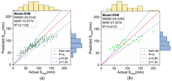
Figure 10.
Prediction results for the SVM model: (a) training set, and (b) test set.
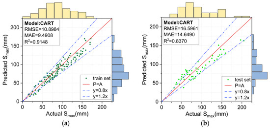
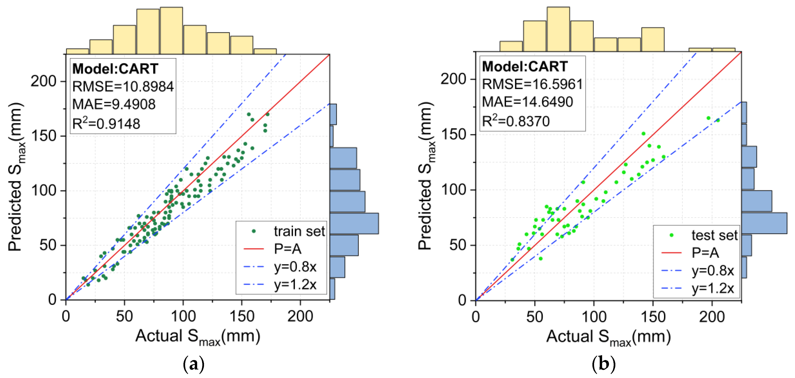
Figure 11.
Prediction results for the CART model: (a) training set, and (b) test set.
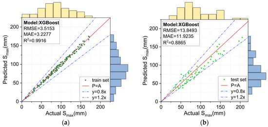
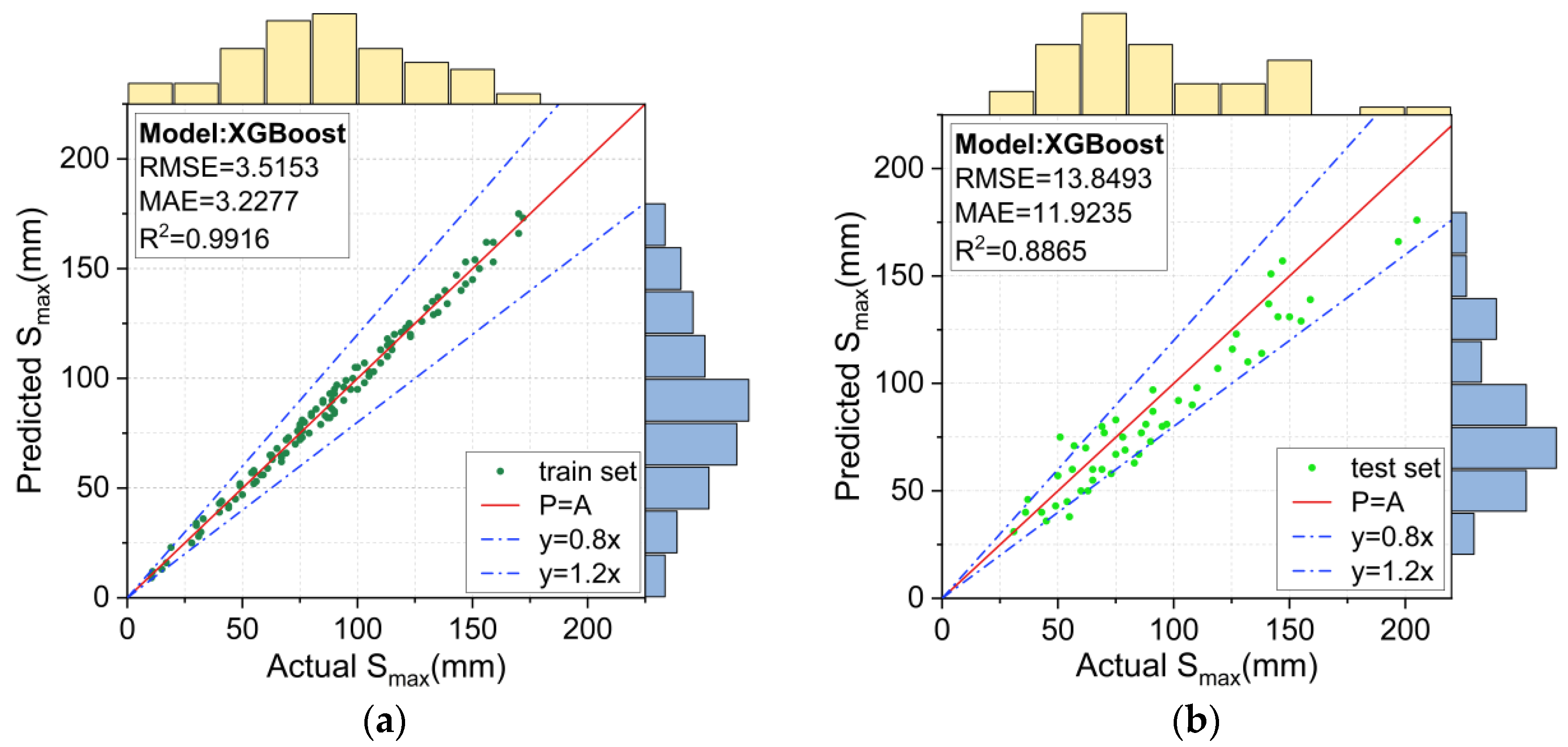
Figure 12.
Prediction results for the XGBoost model: (a) training set, and (b) test set.
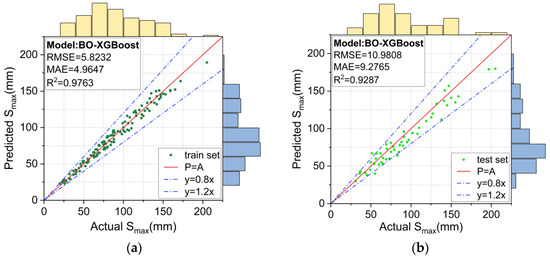
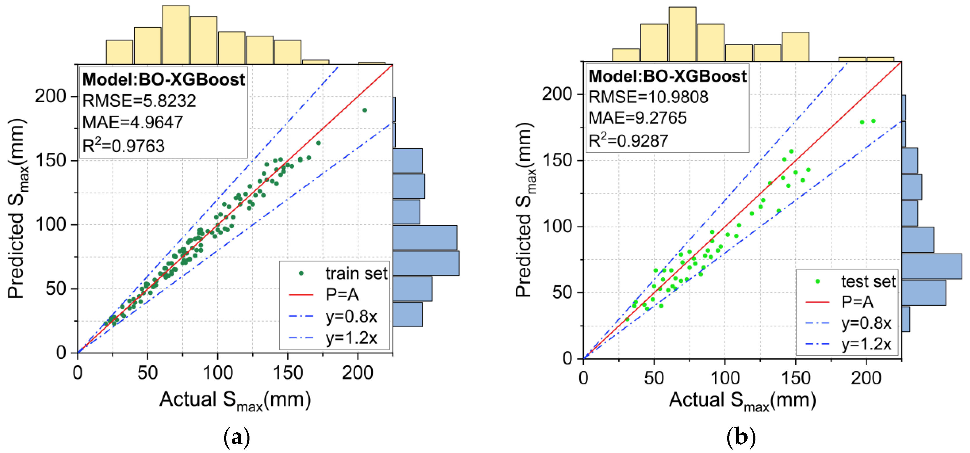
Figure 13.
Prediction results for the BO-XGBoost model: (a) training set, and (b) test set.
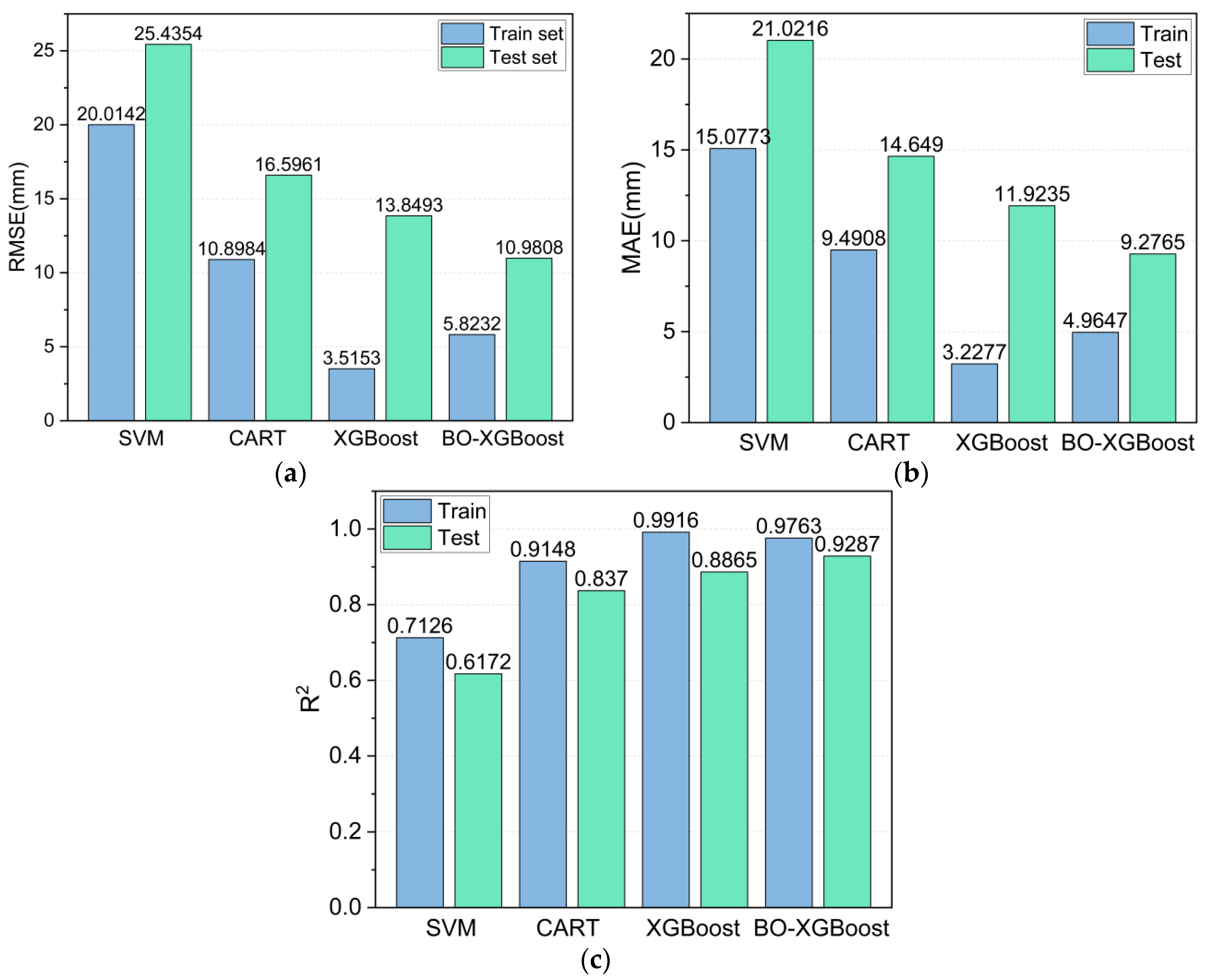
Figure 10a,b shows the prediction results for the training and test sets using the SVM model. The predictions exhibited a clear tendency: the prediction was generally large for smaller measured Smax values and smaller for larger measured Smax values. The RMSE, MAE and R2 values were 20.0142, 15.0773, and 0.7126 for the training set and 25.4354, 21.0216, and 0.6172 for the test set, respectively. This indicated that the prediction results of the SVM model deviated significantly from the measured Smax values, and thus, they were not reliable.
The Smax value predicted by the CART model is plotted in Figure 11. Compared with the SVM model, the CART model could predict a wider range of measured Smax values more accurately. The RMSE, MAE and R2 values of the SVM model for the training set were 10.8984, 9.4908, and 0.9148, respectively, indicating that the predicted values for the entire training set were closer to the measured Smax value. However, the deviation of the CART model was still relatively large for the test set (RMSE = 16.5961 and MAE = 14.6490).
The prediction results using the unoptimized XGBoost model and the BO-XGBoost model are respectively shown in Figure 12 and Figure 13. For the training set, the RMSE, MAE and R2 values were 3.5153, 3.2277, and 0.9916, respectively, for the XGBoost model and 5.8232, 4.9647, and 0.9763, respectively, for the BO-XGBoost model, and they both demonstrated excellent learning abilities for the data. Figure 12a and Figure 13a show the scatter distributions over the range of 0.8 to 1.2 for the accuracy of the P = A line. For the test set, the RMSE and MAE values were reduced from 13.8493 and 11.9235 to 10.9808 and 9.2765, respectively, after the hyperparameters of the XGBoost model were optimized by the Bayesian algorithm. The prediction accuracy of the XGBoost model evaluated by the RMSE and MAE values had improved by 20% and 22%, respectively.
The metrics of the different models evaluated on the training and test sets are summarized in Figure 14 to compare their performances more visually. The models were ranked according to their learning ability on the training set from lowest to highest, as follows: SVM < CART < BO-XGBoost < XGBoost, and, similarly, for their predictive ability on the test set, they were ranked as follows: SVM < CART < XGBoost < BO-XGBoost. Unexpectedly, the BO-XGBoost model showed a lower performance on the training set compared to the unoptimized XGBoost model, but it achieved a better prediction performance on the test set (XGBoost: R2 = 0.8865 and BO-XGBoost: R2 = 0.9287). This could be explained by the fact that the unoptimized XGBoost model tended to overfit the training data, highlighting the importance of hyperparameter optimization for the XGBoost model.

Figure 14.
Model evaluation indexes: (a) RMSE, (b) MAE, and (c) R2.
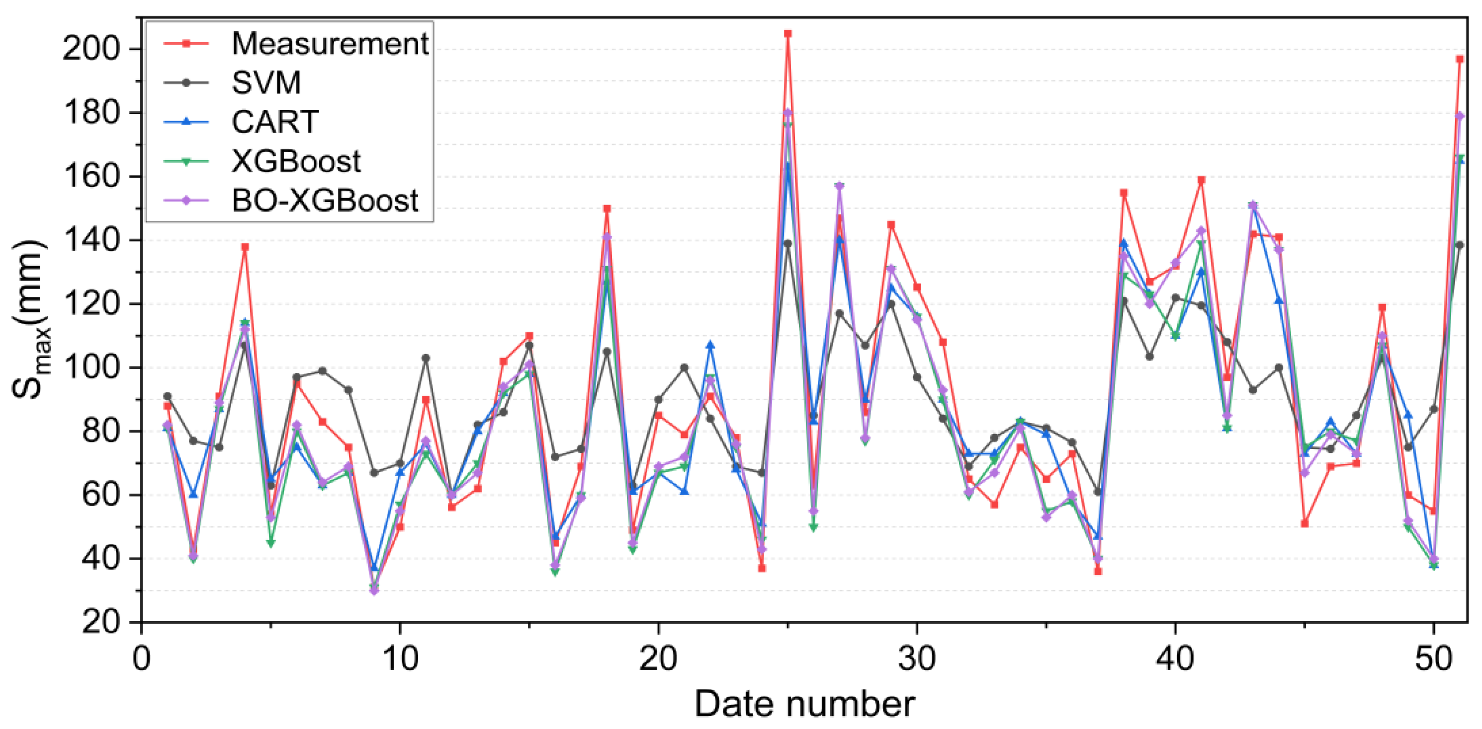
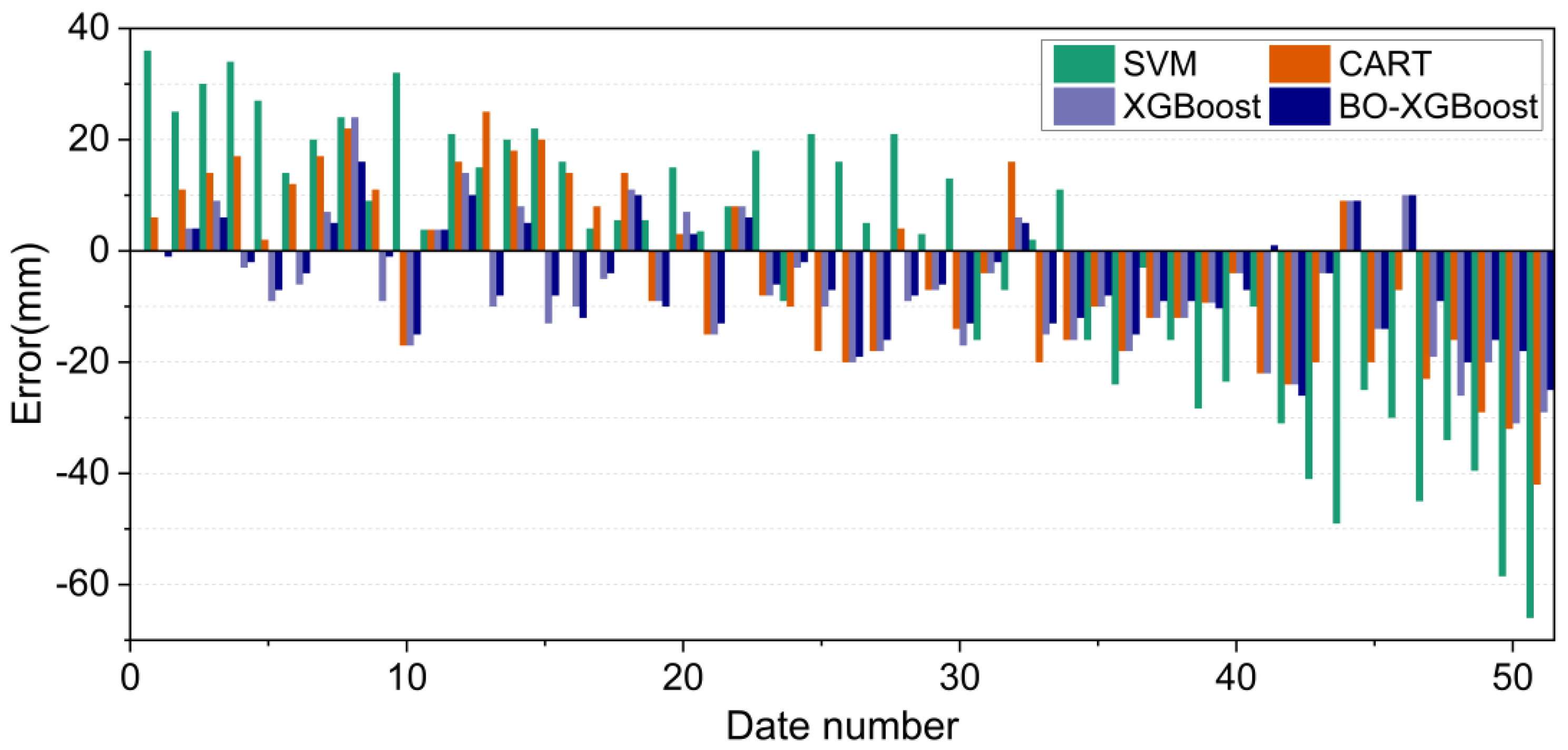
The calculation results of the four algorithm models on the test set are shown in Figure 15. The maximum displacements of the tunnel vault uplift, i.e., the Smax values, were sorted from smallest to largest, and then the errors for the predicted and measured values were calculated using Equation (10):
where represents the predicted uplift displacement and represents the measured uplift displacement. Figure 16 shows the predicted errors corresponding to the four different algorithmic models. The positive values indicate that the predicted value of Smax was greater than the measured value while a negative value indicates the opposite.

Figure 15.
Prediction comparison results for the four algorithmic models on the test set.

Figure 16.
Prediction error results for the four algorithmic models on the test set.
Combining Figure 15 and Figure 16, it can be noticed that the four models exhibited similar prediction patterns, with variations in their accuracy levels. Notably, the SVM model demonstrated the highest deviation from the measured Smax value, with the maximum error exceeding −60 mm, particularly for the highest measured Smax value. This finding highlighted the unsuitability of the SVM model for projects where Smax values are expected to be relatively large, which could potentially compromise engineering safety.
Compared with the SVM model, the prediction accuracy of the CART algorithm model for Smax values had improved, and the maximum prediction error was less than −50 mm. The XGBoost algorithm model provided a more accurate prediction for the measured Smax values than the SVM and CART models, as evidenced by the maximum prediction error value of −31 mm. Meanwhile, the maximum prediction error of the BO-XGBoost algorithm was further reduced to −26 mm, and the absolute value of the maximum prediction error was controlled within 20 mm in most periods. Consequently, the BO-XGBoost algorithm demonstrated the highest prediction accuracy among the four models considered in this study.
Summarizing the above analysis, the BO-XGBoost algorithm model performed better for generalization ability, with a higher prediction accuracy in predicting the maximum uplift displacement of the underlying tunnel vault caused by the excavation, and the prediction error of the maximum uplift displacement was only approximately ±10 mm, which was suitable for practical projects. It is worth noting that for the prediction results of the BO-XGBoost model on the test set, two of the prediction errors exceeded −20 mm and the predicted values were smaller than the measured values. Since the outliers of input variables can provide some extreme information to an established prediction model, the processing of a database in combination with field knowledge is necessary before training a model. However, the overall results demonstrated that the proposed BO-XGBoost model was effective at accurately predicting the maximum tunnel uplift displacement.
4.4. Interpretability of the Prediction Model
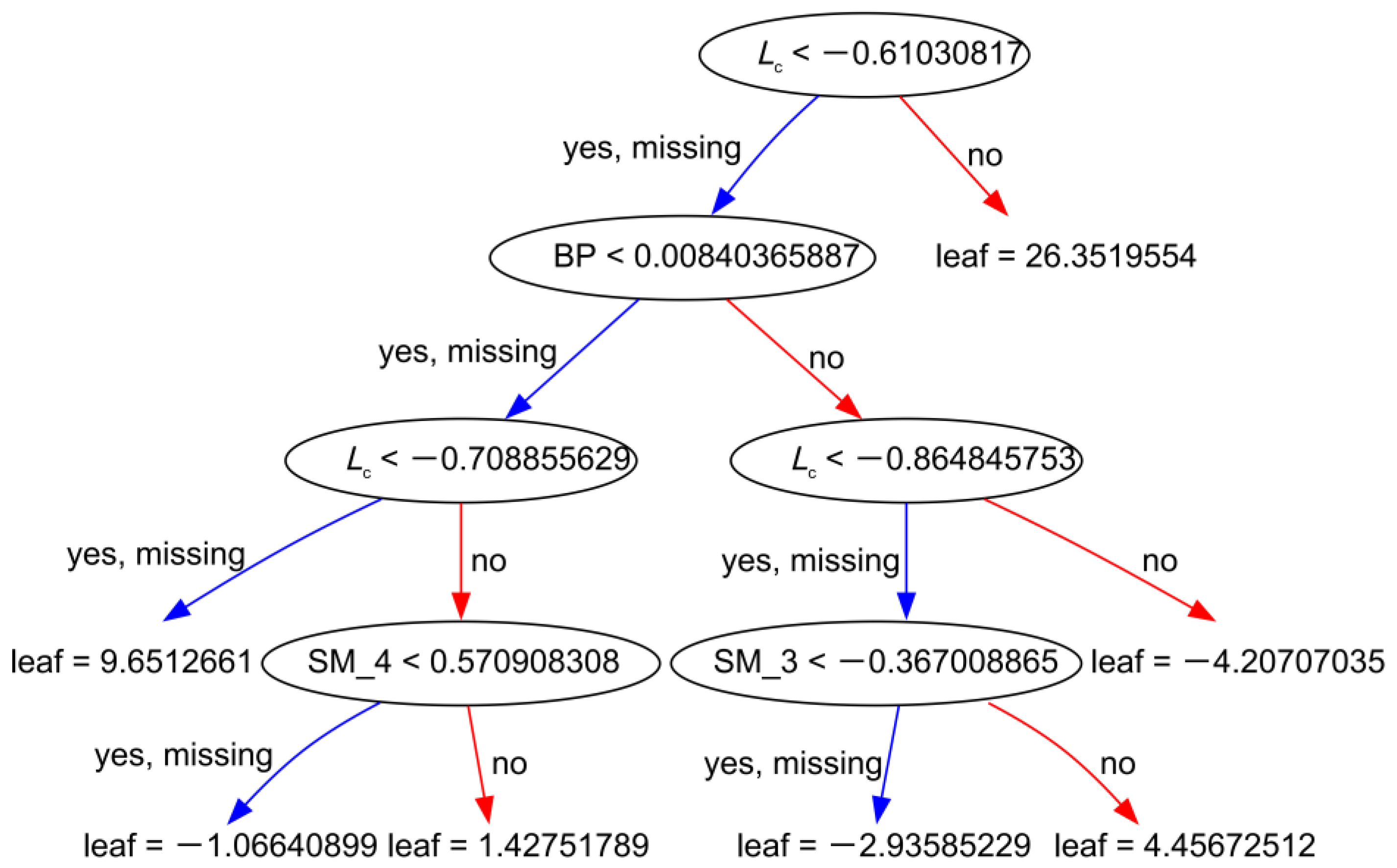
The uplifting behavior of overlying excavations on existing tunnels is a complex civil engineering problem. Explainability is an important criterion for assessing whether or not machine learning models are trustworthy. In other words, a model should not only provide accurate predictions to engineers but also provide a safe and reliable basis for decision-making. The XGBoost model, for example, provided an interface for visualizing decision trees. This feature enhances the interpretability of a model by providing engineers with an intuitive representation of the decision-making process. Figure 17 illustrates the visualization of the last tree by specifying the parameter “num_trees”. This shows that the model consisted of five layers, including four layers of tree structure and one layer of leaf structure, and the features at the nodes determined the cut of the nodes. This visualization capability of the XGBoost model aided in model analysis and provided valuable insights into the decision-making process. It enhanced the model’s explainability, which will allow engineers to understand how a model arrives at its predictions, thereby enabling informed decision-making based on a safe and reliable foundation.
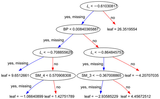
Figure 17.
The XGBoost model’s tree structure.
Feature importance plays a crucial role in elucidating a model’s behavior. By utilizing the feature importance module within the XGBoost model, the proportionate significance levels of the top ten features were calculated according to the number of times they were utilized for splitting the tree. Figure 18 shows the feature importance of the prediction model based on the BO-XGBoost model for the maximum displacement of the tunnel vault uplift.
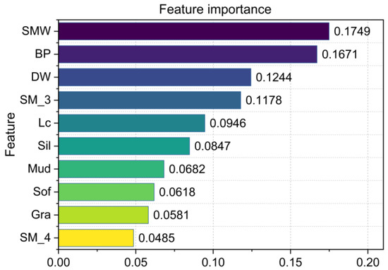
Figure 18.
Feature importance of the BO-XGBoost model.
According to the weight of the feature importance, the three factors SWM, BP, and DW were the most prominent. This indicated that the excavation enclosure structures were the most important factors in this prediction model. Additionally, the remaining features, in descending order of their weight shares, included SM_3, Lc, Sil, Mud, Sof, Gra, and SM_4. The control measure of using uplift-resistant piles (SM_3) in the excavation could effectively control the soil uplift below the excavation bottom. Prior to designing an excavation, equal attention should be given to the actual length (Lc) of a tunnel’s under-crossing. Unexpectedly, the four soil types were ranked at the bottom according to their weights, which were far below the construction measures. This confirmed that suitable construction measures can significantly counteract the effects of geological factors resulting from underlying tunnel uplift. As a result, the interpretability of the BO-XGBoost model provided significant guidance to the tunnel engineers in the decision-making process.
5. Conclusions
This study proposed the XGBoost model in a machine learning algorithm to predict the maximum uplift displacement of an underlying shield tunnel vault caused by an excavation. Meanwhile, the Bayesian optimization algorithm was applied to optimize the XGBoost model’s hyperparameters, and the best prediction model was established, namely, the BO-XGBoost model. The RMSE, MAE, and R2 values were selected as metrics for quantitatively evaluating the prediction performances of the SVM, CART, XGBoost, and BO-XGBoost models. The main conclusions were as follows:
- (1)
- Among the four algorithmic models for Smax prediction, the SVM model’s predicted results deviated the most from the measured values (RMSE = 25.4354, MAE = 21.0216, and R2 = 0.6172). The highest prediction accuracy was achieved by the BO-XGBoost model. In addition, compared to the unoptimized XGBoost model, the RMSE and MAE values of the BO-XGBoost model improved from 13.8493 and 11.9235 to 10.9808 and 9.2765, respectively.
- (2)
- According to the prediction results for the test set, the prediction errors of the four models showed tendencies to grow larger as Smax values grew larger in certain time periods. These tendencies were particularly reflected in the SVM and CART models. The maximum prediction error of the SVM-based model was more than −60 mm, whereas it was near −50 mm for the CART model. However, the maximum prediction error of the BO-XGBoost model was controlled to within ±2 mm for most time periods, which was superior to the ±31 mm error of the XGBoost model.
- (3)
- The BO-XGBoost model had better interpretability, including its ability to visualize the decision trees and calculate the feature importance. According to the weights of the characteristic importance elements, the three measures of the excavation enclosure, in order of the SWM, BP, and DW, were the most critical factors in predicting the maximum tunnel uplift displacement.
- (4)
- Expanding a dataset is beneficial for improving the prediction accuracy of a model. Currently, cases of actual projects with excavations over existing tunnels are insufficient. Apart from this, the input parameters of the training prediction model were still divided in inadequate detail. These play vital roles in achieving higher levels of accuracy for predictive models.
Author Contributions
Conceptualization, H.Z.; methodology, H.Z., Y.W. and P.G.; software, H.Z. and Y.W.; data curation, H.Z.; visualization, X.L.; writing—original draft, H.Z.; writing—review and editing, H.Z. and H.L.; funding acquisition, Y.W. and P.G.; supervision, Y.W. and H.L. All authors have read and agreed to the published version of the manuscript.
Funding
This paper was supported by the National Natural Science Foundation of China grant number 42077249 and 42107082, the opening project of the State Key Laboratory of Explosion Science and Technology (Beijing Institute of Technology), grant number KFJJ23-05M, and the Fundamental Research Funds for the Central Universities, grant number JZ2023HGTA0193 and JZ2023HGQA0094.
Institutional Review Board Statement
Not applicable.
Informed Consent Statement
Not applicable.
Data Availability Statement
Data will be made available upon request.
Conflicts of Interest
The authors declare that they have no known competing financial interests or personal relationships that could have appeared to influence the work reported in this paper.
References
- Zhang, X.M.; Ou, X.F.; Yang, J.S.; Fu, J.Y. Deformation Response of an Existing Tunnel to Upper Excavation of Foundation Pit and Associated Dewatering. Int. J. Geomech. 2017, 17, 04016112. [Google Scholar]
- Zheng, G.; Pan, J.; Li, Y.L.; Cheng, X.S.; Tan, F.L.; Du, Y.M.; Li, X.H. Deformation and protection of existing tunnels at an oblique intersection angle to an excavation. Int. J. Geomech. 2020, 20, 05020004. [Google Scholar] [CrossRef]
- Wei, G.; Feng, F.F.; Hu, C.B.; Zhu, J.X.; Wang, X. Mechanical performances of shield tunnel segments under asymmetric unloading induced by pit excavation. J. Rock Mech. Geotech. Eng. 2022, 15, 1547–1564. [Google Scholar]
- Meng, F.Y.; Chen, R.P.; Xu, Y.; Wu, K.; Wu, H.N.; Liu, Y. Contributions to responses of existing tunnel subjected to nearby excavation: A review. Tunn. Undergr. Space Technol. 2022, 119, 104195. [Google Scholar]
- Zhao, Y.R.; Chen, X.S.; Hu, B.; Wang, P.H.; Li, W.S. Evolution of tunnel uplift induced by adjacent long and collinear excavation and an effective protective measure. Tunn. Undergr. Space Technol. 2023, 131, 104846. [Google Scholar] [CrossRef]
- Sun, H.S.; Chen, Y.D.; Zhang, J.H.; Kuang, T.S. Analytical investigation of tunnel deformation caused by circular foundation pit excavation. Comput. Geotech. 2019, 106, 193–198. [Google Scholar]
- Liang, R.Z.; Wu, W.B.; Yu, F.; Jiang, G.S.; Liu, J.W. Simplified method for evaluating shield tunnel deformation due to adjacent excavation. Tunn. Undergr. Space Technol. 2018, 71, 94–105. [Google Scholar]
- Zhou, Z.; Zhou, X.; Li, L.; Liu, X.; Wang, L.; Wang, Z. The Construction Methods and Control Mechanisms for Subway Station Undercrossing an Existing Tunnel at Zero Distance. Appl. Sci. 2023, 13, 8826. [Google Scholar] [CrossRef]
- Attewell, P.B.; Yeates, J.; Selby, A.R. Soil Movements Induced by Tunnelling and their Effects on Pipelines and Structures. Int. J. Rock Mech. Min. Sci. Geomech. Abstr. 1986, 24, 163. [Google Scholar]
- Bjerrum, L.; Eide, O. Stability of strutted excavations in clay. Géotechnique 2008, 6, 32–47. [Google Scholar] [CrossRef]
- Zong, X. Study of longitudinal deformation of existing tunnel due to above excavation unloading. Rock Soil Mech. 2016, 37 (Suppl. S2), 571–577. [Google Scholar]
- Liu, J.W.; Shi, C.H.; Lei, M.F.; Cao, C.Y.; Lin, Y.X. Improved analytical method for evaluating the responses of a shield tunnel to adjacent excavations and its application. Tunn. Undergr. Space Technol. 2020, 98, 103339. [Google Scholar] [CrossRef]
- Chen, K.; Xu, R.Q.; Ying, H.W.; Liang, R.Z.; Lin, C.G.; Gan, X.L. Simplified method for evaluting deformation responses of existing tunnels due to overlying basement excavation. Chin. J. Rock. Mech. Eng. 2020, 39, 637–648. [Google Scholar]
- Qiu, J.T.; Jiang, J.; Zhou, X.J.; Zhang, Y.F.; Pan, Y.D. Analytical solution for evaluating deformation response of existing metro tunnel due to excavation of adjacent foundation pit. J. Cent. South Univ. 2021, 28, 1888–1900. [Google Scholar]
- Guo, P.P. Characteristics and Control Method for Deformation of Shallowly Buried Pipeline Induced by Braced Excavation. Ph.D. Thesis, Zhejiang University, Zhejiang, China, 2022. [Google Scholar]
- Loganathan, N.; Poulos, H.G. Analytical prediction for tunneling-induced ground movements in clays. J. Geotech. Geoenviron. Eng. 1998, 124, 846–856. [Google Scholar] [CrossRef]
- Lo, K.Y.; Ramsay, J.A. The effect of construction on existing subway tunnels—A case study from Toronto. Tunn. Undergr. Space Technol. 1991, 6, 287–297. [Google Scholar] [CrossRef]
- An, L.; Zheng, G.; Wei, S.W. Effect of dewatering of foundation pits on soil deformation behavior. Chin. J. Geotech. Eng. 2008, 30 (Suppl. S1), 493–498. [Google Scholar]
- Fellin, W.; King, J.; Kirsch, A.; Oberguggenberger, M. Uncertainty modelling and sensitivity analysis of tunnel face stability. Struct. Saf. 2010, 32, 402–410. [Google Scholar] [CrossRef]
- Liu, B.; Zhang, D.W.; Yang, C.; Zhang, Q.B. Long-term performance of metro tunnels induced by adjacent large deep excavation and protective measures in Nanjing silty clay. Tunn. Undergr. Space Technol. 2020, 95, 103147. [Google Scholar]
- Shi, J.W.; Ding, C.; Wu, C.W.; Lu, H.; Chen, L. Effects of overconsolidation ratio on tunnel responses due to overlying basement excavation in clay. Tunn. Undergr. Space Technol. 2020, 97, 103247. [Google Scholar] [CrossRef]
- Zhang, Q.; Tao, Z.G.; Yang, C.; Guo, S.; He, M.C.; Zhang, C.Y.; Niu, H.Y.; Wang, C.; Wang, S. Experimental and numerical investigation into the non-explosive excavation of tunnels. J. Rock Mech. Geotech. Eng. 2022, 14, 1885–1900. [Google Scholar] [CrossRef]
- Doležalová, M. Tunnel complex unloaded by a deep excavation. Comput. Geotech. 2001, 28, 469–493. [Google Scholar] [CrossRef]
- Chen, X.; Guo, H.Y.; Zhao, P.; Peng, X.; Wang, S.Z. Numerical modeling of large deformation and nonlinear frictional contact of excavation boundary of deep soft rock tunnel. J. Rock Mech. Geotech. Eng. 2011, 3 (Suppl. S1), 421–428. [Google Scholar]
- Liu, H.L.; Li, P.; Liu, J.Y. Numerical investigation of underlying tunnel heave during a new tunnel construction. Tunn. Undergr. Space Technol. 2011, 26, 276–283. [Google Scholar] [CrossRef]
- Li, J.J.; Chen, J.S.; Liu, S.Z.; Mo, H.H. Study on Protection Measures of Excavation above the Nearby Metro. Chin. J. Undergr. Space Eng. 2016, 12 (Suppl. S1), 348–353. [Google Scholar]
- Estahbanati, S.H.; Boushehri, R.; Soroush, A.; Ghasemi-Fare, O. Numerical Analysis of Dynamic Response of Lifelines Facilities Adjacent to Deep Excavations. In Proceedings of the Geo-Congress 2020: Geotechnical Earthquake Engineering and Special Topics, Minneapolis, MN, USA, 21 February 2020. [Google Scholar]
- Zhang, W.G.; Li, H.R.; Wu, C.Z.; Li, Y.Q.; Liu, Z.Q.; Liu, H.L. Soft computing approach for prediction of surface settlement induced by earth pressure balance shield tunneling. Undergr. Space 2021, 6, 353–363. [Google Scholar] [CrossRef]
- Chen, R.P.; Dai, T.; Zhang, P.; Wu, H.N. Prediction Method of Tunneling-induced Ground Settlement Using Machine Learning Algorithms. J. Hunan Univ. Nat. Sci. 2021, 48, 111–118. [Google Scholar]
- Shi, J.S.; Ortigao, J.A.R.; Bai, J.L. Modular neural networks for predicting settlements during tunneling. J. Geotech. Geoenviron. Eng. 1998, 124, 389–395. [Google Scholar] [CrossRef]
- Kim, C.Y.; Bae, G.J.; Hong, S.W.; Park, C.H.; Moon, H.K.; Shin, H.S. Neural network based prediction of ground surface settlements due to tunnelling. Comput. Geotech. 2001, 28, 517–547. [Google Scholar] [CrossRef]
- Leu, S.S.; Lo, H.C. Neural-network-based regression model of ground surface settlement induced by deep excavation. Autom. Constr. 2004, 13, 279–289. [Google Scholar]
- Suwansawat, S.; Einstein, H.H. Artificial neural networks for predicting the maximum surface settlement caused by EPB shield tunneling. Tunn. Undergr. Space Technol. 2006, 21, 133–150. [Google Scholar] [CrossRef]
- Chen, Y.L.; Azzam, R.; Fernandez-Steeger, T.M.; Li, L. Studies on construction pre-control of a connection aisle between two neighboring tunnels in Shanghai by means of 3D FEM, neural networks and fuzzy logic. Geotech. Geol. Eng. 2009, 27, 155–167. [Google Scholar] [CrossRef]
- Zhou, Y.; Li, S.Q.; Zhou, C.; Luo, H.B. Intelligent Approach Based on Random Forest for Safety Risk Prediction of Deep Foundation Pit in Subway Stations. J. Comput. Civil Eng. 2019, 33, 05018004. [Google Scholar] [CrossRef]
- Zhang, D.M.; Shen, Y.M.; Huang, Z.K.; Xie, X.C. Auto machine learning-based modelling and prediction of excavation-induced tunnel displacement. J. Rock Mech. Geotech. Eng. 2022, 14, 1100–1114. [Google Scholar] [CrossRef]
- Li, W.D.; Wu, M.H.; Lin, N. Horizontal displacement prediction research of deep foundation pit based on the least square support vector machine. In Proceedings of the 3rd International Conference on Wireless Communication and Sensor Networks, Wuhan, China, 10–11 December 2016. [Google Scholar]
- Li, X.; Li, X.B.; Su, Y.H. A hybrid approach combining uniform design and support vector machine to probabilistic tunnel stability assessment. Struct. Saf. 2016, 61, 22–42. [Google Scholar] [CrossRef]
- Zhou, Y.; Su, W.; Ding, L.Y.; Luo, H.B.; Love, P.E.D. Predicting safety risks in deep foundation pits in subway infrastructure projects: A support vector machine approach. J. Comput. Civil Eng. 2017, 31, 04017052. [Google Scholar] [CrossRef]
- Yao, B.Z.; Yang, C.Y.; Yao, J.B.; Sun, J. Tunnel surrounding rock displacement prediction using support vector machine. Int. J. Comput. Intell. Syst. 2010, 3, 843–852. [Google Scholar]
- Nanni, L.; Lumini, A. An experimental comparison of ensemble of classifiers for bankruptcy prediction and credit scoring. Expert Syst. Appl. 2009, 36, 3028–3033. [Google Scholar] [CrossRef]
- Lessmann, S.; Baesens, B.; Seow, H.V.; Thomas, L.C. Benchmarking state-of-the-art classification algorithms for credit scoring: An update of research. Eur. J. Oper. Res. 2015, 247, 124–136. [Google Scholar] [CrossRef]
- Zhou, X.Z.; Zhao, C.; Bian, X.C. Prediction of maximum ground surface settlement induced by shield tunneling using XGBoost algorithm with golden-sine seagull optimization. Comput. Geotech. 2022, 154, 105156. [Google Scholar] [CrossRef]
- Su, J.; Wang, Y.Z.; Niu, X.K.; Sha, S.; Yu, J.Y. Prediction of ground surface settlement by shield tunneling using XGBoost and Bayesian Optimization. Eng. Appl. Artif. Intell. 2022, 114, 105020. [Google Scholar] [CrossRef]
- Chen, T.Q.; Guestrin, C. XGBoost: A scalable tree boosting system. In Proceedings of the 22nd ACM SIGKDD International Conference on Knowledge Discovery and Data, San Francisco, CA, USA, 13–17 August 2016. [Google Scholar]
- Shahriari, B.; Swersky, K.; Wang, Z.Y.; Adams, R.P.; Freitas, N. Taking the human out of the loop: A review of Bayesian optimization. Proc. IEEE 2015, 104, 148–175. [Google Scholar] [CrossRef]


Disclaimer/Publisher’s Note: The statements, opinions and data contained in all publications are solely those of the individual author(s) and contributor(s) and not of MDPI and/or the editor(s). MDPI and/or the editor(s) disclaim responsibility for any injury to people or property resulting from any ideas, methods, instructions or products referred to in the content. |
© 2023 by the authors. Licensee MDPI, Basel, Switzerland. This article is an open access article distributed under the terms and conditions of the Creative Commons Attribution (CC BY) license (https://creativecommons.org/licenses/by/4.0/).