Article

Research on Trajectory Planning and Tracking Methods for Coal Mine Mobile Robots

1
School of Mechatronic Engineering, China University of Mining and Technology, Xuzhou 221116, China
2
Jiangsu Collaborative Innovation Center of Intelligent Mining Equipment, China University of Mining and Technology, Xuzhou 221008, China
3
State Key Laboratory of Robotics, Shenyang Institute of Automation, Chinese Academy of Sciences, Shenyang 110016, China
4
Information Institute, Ministry of Emergency Management of the People’s Republic of China, Beijing 100029, China
*
Author to whom correspondence should be addressed.
Appl. Sci. 2023, 13(17), 9789; https://doi.org/10.3390/app13179789
Submission received: 30 July 2023 / Revised: 22 August 2023 / Accepted: 25 August 2023 / Published: 30 August 2023
(This article belongs to the Section Robotics and Automation)

Abstract

:
Coal Mine Mobile Robots (CMRRs) are generally large in size and inertia, while narrow laneway space and bumpy terrain pose great challenges to CMRR’s planning and control. Aiming at the trajectory planning and tracking problems of CMRR, a new trajectory class MINCO is derived in detail based on the properties of differential flat systems. A trajectory planning method based on MINCO trajectory and safety corridor constraints constructed with underground environmental constraints is further proposed. A trajectory tracking method based on model predictive control (MPC) is further proposed. The prediction model of MPC is constructed by a kinematics model and transformed into a standard quadratic programming problem according to the cost function of a trajectory tracking target. Finally, large quantities of field tests were carried out for the proposed approaches. The results show that the proposed planning algorithm based on MINCO trajectory can achieve good avoidance effects within 10 planning attempts in different obstacle scenarios, and the trajectory is smoother compared to the Fast-Planner algorithm, with shorter trajectory length and less planning time. The tracking error of MPC is always less than 0.05 m in different underground scenarios, having a more adaptable trajectory tracking effect than PID.

1. Introduction

In January 2019, the State Administration of Coal Mine Safety of China released the Key Research and Development Catalog of Coal Mine Robots, proposing to vigorously research and develop the application of coal mine robots to promote the high-quality development of the coal industry [1]. Underground, tracked mobile robots in coal mines have a wide range of application prospects in the fields of digging, drilling, safety and control, rescue and auxiliary operations, etc. As an important branch of coal mine robots, the application of their autonomous navigation largely responds to the degree of development of the intelligentization of underground operations. Trajectory planning is an important research direction in the field of mobile robotics, and its task is to plan a dynamically feasible desired trajectory based on safety constraints, optimization goals, and other constraints [2]. Trajectory tracking can track the smooth trajectory generated by the trajectory planning module and control the robot to track the target trajectory by solving the appropriate control quantity of the robot through the relevant algorithm. Trajectory planning and trajectory tracking are the keys for CMRRs to realize autonomous navigation [3]. Most of the underground coal mine environments are unstructured and complex terrains, with narrow space and the presence of many obstacles such as debris and coal blocks, so the application of robot trajectory planning and tracking puts forward higher requirements. How to apply trajectory planning and tracking technology to mobile robots in underground coal mines is of great significance for the development of “unmanned and intelligent” coal mine mobile equipment, improving the reliability and safety of coal mine robots, and reducing the rate of accidents in coal mine fields.
Trajectory planning is usually divided into two parts: front-end path planning and back-end speed planning. Front-end path planning methods include search-based methods, sampling-based methods, etc. Back-end speed planning involves carrying out path smoothing and speed planning on the basis of better paths obtained from front-end path planning, and the commonly used methods include polynomial-based trajectory planning methods and Bessel curve-based trajectory planning methods. Bao et al. [4] improved and fused the A* algorithm and artificial potential field algorithm, which was successfully applied to the path planning of underground, trackless, rubber-wheeled vehicles. Sampling-based methods include the Probabilistic Roadmap (PRM) [5] and Rapidly Exploring Random Trees (RRT) [6]. In response to the non-optimality of the sampling algorithm, Karaman and Frazzoli proposed an improved algorithm for RRT, called RRT* algorithm, which combines the asymptotic optimality of the Rapidly Exploring Random Graph (RRG) [7] while maintaining a tree structure like RRT to ensure that the RRT* algorithm can quickly converge to an optimal path solution. Yan et al. [8] designed a quintic polynomial-based trajectory planning method based on the requirements of trajectory smoothness and efficiency when self-driving vehicles change lanes; designed the cost function with the objective of minimizing the average curvature and shortest length of the trajectory; used the vehicle linear velocity, angular velocity, and other constraints as constraints; and finally, the trajectory was solved by a sequential quadratic programming algorithm. Bezier curves have been widely used in trajectory generation for autonomous driving systems because of features such as smooth lines [9,10]. Choi et al. [11] proposed two third-order Bezier curve-based trajectory planning algorithms for autonomous vehicle trajectory generation under waypoint and road boundary constraints. Bae et al. [12] analyzed that the minimum order of a Bessel curve that can satisfy the condition that the curvature value of the start point and the end point are both zero is the fifth order, and a feasible trajectory planning algorithm for intelligent cars is proposed based on the fifth order Bessel curve. Qu et al. [13] established a step-by-step planning model based on B spline curves and verified through simulation that the method can better solve the intelligent vehicle trajectory planning problem under simple obstacle scenarios. Maekawa et al. [14] generated executable paths with continuous curvature based on cubic B spline curves for unmanned vehicles in mineral operations. Zhu et al. [15] present a trajectory optimization method by parameterized curvature control to reach the goal state with the vehicle model and its dynamic constraints considered to deal with the highly dynamic environments for on-road automotive driving.
Trajectory tracking is the basis for robots to be able to accomplish various tasks such as autonomous navigation and movement in unknown and complex environments. However, mobile robots are inherently characterized by noncomplete constraints and strong nonlinearities [16], which make it difficult to control them well. The task of trajectory tracking is to output appropriate control quantities according to the real-time position and model constraints of the robot, so that the actual position of the robot is consistent with the position on the target trajectory, and its commonly used methods include PID control, sliding mode control (SMC), and MPC control. Zhu et al. [17] used a fuzzy adaptive PID control algorithm to track and control the trajectory of AGV to improve the trajectory tracking accuracy in response to the problems of low running accuracy and long PID control adjustment time when the Automated Guided Vehicle (AGV) is performing circular motion. Li et al. [18] based a trajectory tracking controller on visual neuron PID, so that the robot can meet the robustness of the tracking controller even when it makes a rapid response. Thi et al. [19] proposed an algorithm combining the backstepping technique and sliding mode control for trajectory tracking of four-wheeled omni-directional mobile robots, so that the robots can track any type of trajectory. Jun et al. [20] designed an adaptive trajectory tracking controller based on sliding film feedback for tracked mobile robots to improve the trajectory tracking accuracy of tracked mobile robots. Minh et al. [21] designed a nonlinear MPC control algorithm for controlling the robot to track the feasible paths generated directly by nonlinear dynamics equations. Li et al. [22] established a three-degree-of-freedom dynamics model of a vehicle and designed an MPC controller based on it to improve the trajectory tracking accuracy of an intelligently driven vehicle under extreme operating conditions. Shi et al. [23] designed a trajectory tracking controller for intelligent vehicles based on MPC and fuzzy control, and verified in simulation that this method has a good tracking effect under high-speed working conditions. Boryga et al. [24] present a method of bicurve polynomial transition curve application for making agricultural aggregate movement paths during headland turn drives as well as within the field.
In summary, among the current trajectory planning methods, the polynomial spline, the Bézier curve, or B-spline methods have a more flexible trajectory characterization than other traditional methods, but the continuity, parameter dimensions, and the degree of difficulty of implementation still can be improved. Compared to PID and SMC, MPC can handle nonlinear systems and high-order systems, which is more suitable for CMRRs in complex environments. From the analysis of the current situation, it can be found that most of the current trajectory planning and tracking studies are for ground robots, and there are few trajectory planning and tracking studies based on coal mine robots considering the special underground environment. In this paper, we propose a trajectory planning algorithm based on MINCO trajectory and safety corridors for tracked coal mine robots and underground environments, combine it with the MPC trajectory tracking method to complete the overall program design of trajectory planning and tracking for tracked CMRRs, and finally verify the feasibility of the program through experiments.

2. Trajectory Planning Based on MINCO Trajectory Classes

2.1. Differential Flatness-Based Control Optimization Trajectories

In traditional trajectory planning, multidimensional trajectory problems can usually only be solved by solving multiple dimensions separately. Fliess et al. first proposed the concept of differential flatness for nonlinear systems [24], and it was valued in the field of robotic trajectory planning in the following years [25,26,27]. The differential flatness property is conducive to lowering the dimensionality in the optimization problem, decreasing the number of operations, and increasing the efficiency of the computation. Therefore, it has high application value in trajectory planning. The kinematic model of the downhole mobile robot used in the experiment will be given in the later section, and its differential flatness will be verified, so the differential flatness and its application in trajectory planning will be directly discussed first.

2.1.1. Differential Flatness System

For a control system, it can usually be represented in the following form:
x ˙ = f ( x , u ) , x R n , u R m
z = g ( x ) , z R m
where x is the state variable, u is the control variable, z is the output variable, and f and g are the corresponding mappings. A differential flat system is defined as follows: if the state variables and input variables of a system can be determined by the output variables and their finite element derivatives, then the system is a differential flat system. If the system expressed in Equations (1) and (2) is a differential flat system, then x and u can be expressed by the finite element derivatives of z :
x = Ψ x ( z , z ˙ , , z ( s 1 ) )
u = Ψ u ( z , z ˙ , , z ( s ) )
where Ψ x and Ψ u can be determined from f and g. If the outputs are known, all the system variables can be determined without combining system Equations (1) and (2). The differential flatness property can be easily utilized to satisfy the constraints of the system equations and state variables, control variables, and output variables during trajectory generation. If a new set of control variables v = z ( s ) is introduced, then define z [ s 1 ] R m s :
z [ s 1 ] = ( z T , z ˙ T , , z ( s 1 ) T ) T
In this way, the control variables u = Ψ u ( z [ s 1 ] , v ) can decouple the original differential flat system into an integral chain with m dimension [28]. z i and v i are used to denote the I dimension of z and v; denoting the ith dimension in z and v by z i and v i , respectively, the ith integral chain can be expressed as:
z ˙ i [ s 1 ] = 0 I s 1 0 0 T z i [ s 1 ] + 0 1 v i
where I and 0 are the unit and zero matrices with appropriate dimensions. If the initial and termination states are provided, the boundary conditions for the integral chain shown in Equation (6) can be computed. Finally, all state trajectories and control inputs satisfying the original system equations are obtained by integrating the output trajectories obtained from this m-dimensional integration chain and Equations (3) and (4).

2.1.2. Trajectory Optimization in Flat Space

Denote the flat output of the mobile robot as z ( t ) [ 0 , T ] R m . In order to generate usable trajectories for the mobile robot, the trajectories in a flat output space are straightforward optimized, and appropriate constraints are assigned with them (safety constraints and human-defined constraints). The state trajectories x ( t ) and control trajectories u ( t ) of the whole system are then obtained using Ψ x and Ψ u for flat mapping relations for z ( t ) .
In order to make the planned trajectory as smooth as possible, the quadratic planning form of the control quantities is chosen as the cost function to optimize z ( t ) . In order to make the trajectory feasible, the system constraints of the mobile robot are divided into two parts. The first part is the spatial safety constraint, i.e., the trajectory must avoid obstacles to achieve collision-free capabilities, which can be expressed as:
z ( t ) F , t [ 0 , T ]
where F denotes the set of obstacle-free spaces, i.e., the passable area. The second part of the constraints are human-defined dynamic constraints, such as speed and acceleration limits of the robot, which can be expressed as:
G D ( x ( t ) , u ( t ) ) _ 0 , t [ 0 , T ]
Dynamic constraints can be written in the form of representations of z ( t ) by mapping Ψ x and Ψ u :
Ψ x ( z [ s 1 ] ( t ) ) , Ψ u ( z [ s ] ( t ) ) ) _ 0 , t [ 0 , T ]
Differential flatness is then utilized to express the state x ( t ) and control u ( t ) in the form of their finite order derivatives. Then, the constraint of Equation (9) can be expressed as:
G ( z ( t ) , z ˙ ( t ) , , z ( s ) ( t ) ) _ 0 , t [ 0 , T ]
where G is a vector function with dimension related to the customized constraints. In summary, the control cost-optimized trajectory problem with a time-regular term for a differential flat robot system can be described as:
min z ( t ) , T 0 T v ( t ) T W v ( t ) d t + ρ ( T ) ( a ) z ( s ) ( t ) = v ( t ) , t [ 0 , T ] ( b ) G ( z ( t ) , , z ( s ) ( t ) ) _ 0 , t [ 0 , T ] ( c ) z ( t ) F , t [ 0 , T ] ( d ) z [ s 1 ] ( 0 ) = z ¯ 0 , z [ s 1 ] ( T ) = z ¯ f ( e )
where W R m × m is a diagonal matrix with all positive elements, z ¯ 0 R m s is the starting boundary condition of the trajectory, z ¯ f R m s is the terminating boundary condition, and ρ ( T ) is a time regular term which is a positive real number.
Further assumptions on the constraints ρ , G , and F can make the description of problem (11) more concrete. First for the time-regularity term, it can generally be taken as ρ s ( T ) = k ρ T to prevent the trajectory from taking too long to reach the end point, or it can be of the following form to expect the total time of the trajectory to be a deterministic value:
ρ f ( T ) = 0 i f   T = T Σ i f   T T Σ
For a nonlinear constraint G , it is required that it satisfies at least second-order differentiability and continuity. For the constraint space F , it can be approximated as a concatenation of M feasible subregions, i.e.,:
F F ˜ = i M P i
It is also specified that the local connections between these feasible subregions are sequential, i.e.,:
P i P i = Ø i f i j = 2 I n t ( P i P i ) Ø i f i j 1
where I n t ( ) denotes the interior of the set, P 1 and P M denote the initial and terminating subregions, and the boundary conditions z ¯ 0 and z ¯ f are, respectively, in P 1 and P M . If these subregions are spherical regions with m dimensions, the ith subregion can be represented as:
P i B = x R m   x o i 2 r i
It can also be expressed in the more general form of a spatially closed region, i.e., in the form of a convex polyhedron:
P i H = x R m   A i x _ b i
Finally, the description of the trajectory optimization problem in a flat output space is completed.

2.1.3. Multisegment Trajectory Optimization Problem in the Unconstrained Case

For costly optimization of single-segment trajectory control given only a set of initial and termination boundary conditions, commonly used methods include polynomial curve-based and Bessel curve-based trajectory optimization. If the environmental obstacles are complex, the planning results obtained may be more costly or have a smaller safety threshold. If multiple polynomial trajectories are considered, each of which is represented by a polynomial curve, and each of which has a set of boundary conditions, a trajectory with a large safety threshold at a small cost can be obtained as long as the intermediate points are chosen appropriately.
The M segment polynomial trajectory control cost optimization problem for the unconstrained case can be described as Equation (17):
min z ( t ) 0 T v ( t ) T W v ( t ) d t ( a ) z ( s ) ( t ) = v ( t ) , t [ t 0 , t M ] ( b ) z [ s 1 ] ( t 0 ) = z ¯ 0 ,   z [ s 1 ] ( t M ) = z ¯ f ( c ) z [ d i 1 ] ( t i ) = z ¯ i ,   1 i M ( d ) t i 1 < t i ,   1 i M ( e )
where the time region from t 0 to t M is separated into M time segments by M + 1 fixed time points. Each time segment corresponds to a section of the trajectory. The initial and termination conditions of the entire trajectory are represented, respectively, by z ¯ 0 , z ¯ f R m s . z ¯ i R m d i is the intermediate condition and d i s , indicating that the intermediate condition of the derivatives of the 0th to the d i 1 order derivatives needs to be satisfied for z ( t ) at the time t i , i.e., it must satisfy z ( t i ) , z ˙ ( t i ) , , z d i 1 ( t i ) . For example, when d i = 1 , only the 0th order derivative, i.e., the position, is included, which is reflected in the trajectory that the trajectory needs to pass through for this waypoint z ( t i ) , but there is no restriction on the velocity, acceleration, etc., at this point.

2.1.4. Trajectory Optimization Solution without Cost Function

The trajectory z * ( t ) is the optimal solution to problem (17) if the trajectory z * ( t ) : [ t 0 , t M ] satisfies the sufficient and necessary condition for optimality. The optimality condition is described as the optimal solution when z * ( t ) exists and is unique if and only if all the following conditions are satisfied [29]:
  • For any 1 i M , z * ( t ) : [ t i 1 , t i ] is a polynomial with 2s − 1 order;
  • The trajectory z * ( t ) : [ t 0 , t M ] should satisfy formula (17c) and (17d);
  • For any 1 i M , the trajectory z * ( t ) satisfies d ¯ i 1 order continuous differentiability at t i , where d ¯ i = 2 s d i .
By applying the optimality condition, there is a direct way to obtain an optimal trajectory without the aid of a cost function. For an m dimensionally Nth ( N = 2 s 1 ) polynomial trajectory, the segment i can be expressed as:
p i ( t ) = c i T β ( t t i 1 ) , t [ t i 1 , t i ]
where c i R 2 s × m and β ( x ) = ( 1 , x , , x N ) T are the coefficient matrix and basis of the polynomial, respectively. For ease of understanding, the trajectory is represented using relative time, i.e., the timeline t 0 = 0 . A multiband polynomial trajectory can then be represented by a matrix of coefficients c R 2 M s × m and a time vector T R > 0 M :
c = ( c 1 T , , c M T ) T ,   T = ( T 1 , , T M ) T
where T i is the time elapsed in the trajectory of segment i, the total length of the trajectory is T = T 1 . The ith timestamp of the trajectory is the sum of the times of the previous trajectories, i.e., t i = t 1 + t 2 + + t i 1 + t i . Define the M segment polynomial trajectory p : [ 0 , T ] as:
p ( t ) = p i ( t ) , t [ t i 1 , t i ) , i { 1 , , M }
The unique optimal solution to problem (17) can be computed by enforcing the optimality sufficiency and necessary condition on the coefficient matrix c. D 0 , D M R s × m is the initial and termination boundary conditions of the whole trajectory, D i R d i × m is intermediate derivative conditions at the time-stamped t i , and each column of D i is a dimension of the intermediate conditions. Therefore, the intermediate condition at t i can be expressed by the coefficient matrix E i , F i R 2 s × 2 s as follows:
E i F i c i c i + 1 = D i 0 d ¯ i × m
where
E i = ( β ( T i ) , , β d i 1 ( T i ) , β ( T i ) , , β d ¯ i 1 ( T i ) ) T F i = ( 0 , β ( 0 ) , , β d ¯ i 1 ( 0 ) ) T
For the initial and termination boundary conditions of the trajectory, they are E M , F 0 R s × 2 s , expressed as shown below:
F 0 = ( β ( 0 ) , , β ( s 1 ) ( 0 ) ) T E M = ( β ( T M ) , , β ( s 1 ) ( T M ) ) T
Thus, a system of linear equations with respect to the coefficient matrices is obtained by enforcing a sufficient and necessary condition of optimality on the coefficient matrices:
M c = b
The coefficient matrix c solved by this system of equations is the optimal coefficient matrix, where M R 2 M s × 2 M s and b R 2 M s × m are as follows:
M = F 0 0 0 0 E 1 F 1 0 0 0 E 2 F 2 0 0 0 0 F M 1 0 0 0 E M , b = D 0 D 1 0 d ¯ 1 × m D M 1 0 d ¯ M 1 × m D M
The uniqueness of the optimality condition determines the nonsingularity of the matrix M with respect to the time vector T whose elements are all positive, so that the unique optimal solution of the coefficient matrix c can be determined by the system of linear Equation (24). Thus, by means of the optimality condition and the system of Equation (24), and given the boundary conditions D 0 , D M and the intermediate conditions D i , it is possible to obtain the optimal polynomial trajectories with the optimal cost of control for unconstrained conditions without the aid of the cost function, and the computational complexity of the method is linear.

2.1.5. MINCO Trajectory Class

After the analysis of the above content, it can be seen that in the case of certain initial and termination boundary conditions, if a set of intermediate path point vectors q = ( q 1 , , q M 1 ) and the corresponding time vectors T = ( T 1 , , T M ) T of the intermediate paths of the mobile robot trajectories are given (where q i = R m is the 0th-order derivative at the intermediate time point t i , which is the position, and T i is the time interval between t i 1 and t i ), then according to the sufficiency and necessary conditions for optimality the only corresponding multisegment polynomial trajectory with the optimal control cost can be obtained as shown in Figure 1.
Each set of q and T corresponds to a control-optimized multiband polynomial trajectory, and such trajectories are defined as the class of MINCO trajectories, which can be denoted as:
Σ M I N C O = { p ( t ) : [ 0 , T ] | c = c ( q , T ) , q R m × ( M 1 ) , T R > 0 M }
where c = c ( q , T ) is determined by the optimality condition. And the MINCO trajectory can be optimized by spatio-temporal deformation of the cost function in problem (11); the process is roughly as follows: because the cost function of a polynomial trajectory is a function of its coefficient matrix and the time vector, one can denote the artificially-defined cost function or the constraint function as K ( c , T ) , which can be denoted by W ( q , T ) = K ( c ( q , T ) , T ) by MINCO trajectory. Subsequently, as long as W is known and its gradient is 𝜕 W / 𝜕 q , then 𝜕 W / 𝜕 T can optimize the cost function by spatio-temporal deformation of the MINCO trajectory. The computation of W is the positive generating process of MINCO trajectory. The final form of 𝜕 W / 𝜕 q and 𝜕 W / 𝜕 T shows as follows [29]:
𝜕 W 𝜕 q = ( G 1 T e 1 , , G M 1 T e 1 ) 𝜕 W 𝜕 T i = 𝜕 K 𝜕 T i T r { G i T 𝜕 E i 𝜕 T i c i }
𝜕 W / 𝜕 T can be obtained by solving for all 𝜕 W / 𝜕 T i , where 1 i M , and G = ( G 0 T , G 1 T , , G M 1 T , G M T ) T is determined by the following equation:
M T G = 𝜕 K 𝜕 c
M has been shown in (25). T r { } represents the trace of the matrix. E i has been shown in (22). The above computational procedure constitutes a gradient computation of O(M) linear complexity. Thus, the MINCO trajectory can be spatial-temporally deformed to obtain the optimal control trajectory with the given constraints by a generalized solver.

2.2. Trajectory Planning Based on MINCO Trajectories and Safe Corridors

Based on the MINCO trajectory class, the optimal control trajectory of a mobile robot can be obtained in the unconstrained case with given boundary conditions and intermediate conditions. It is necessary to further apply the MINCO trajectory and its spatio-temporal deformation under the constraints of the underground coal mine environment to obtain the optimal motion trajectory suitable for the robot with the optimal control cost, and to propose a trajectory-planning algorithm based on the MINCO trajectory and the safety corridor.

2.2.1. Underground Coal Mine Environmental Constraints and Map Representation

The constraints in trajectory planning in underground environments are mainly safety constraints, i.e., the robot is required to avoid environmental obstacles such as large coal blocks and debris during the planning process.
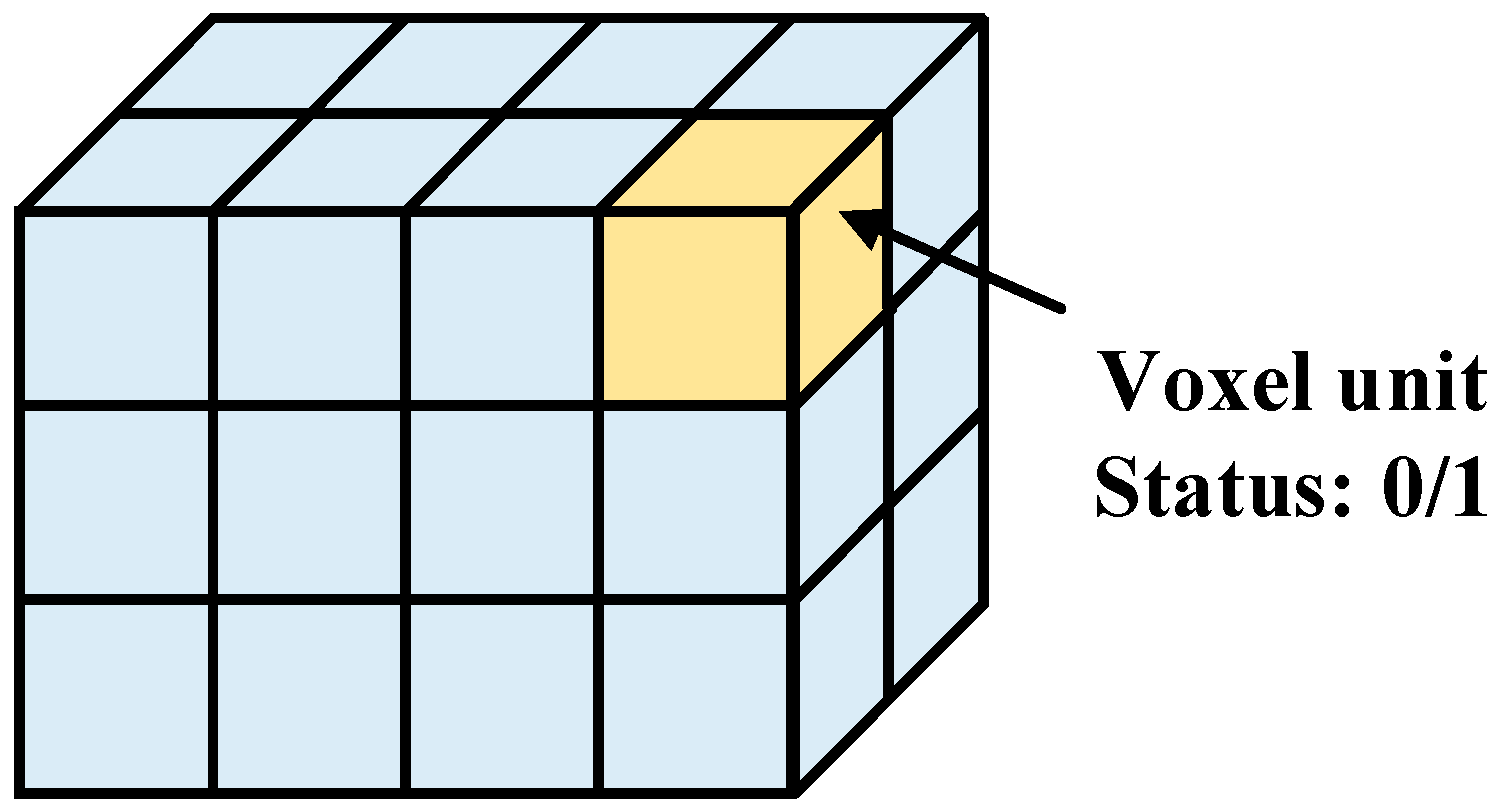
The map used is a voxel map, and the voxels can be viewed as a rough version of the point cloud, as shown in Figure 2. Occupancy information is stored in each voxel cell, and there are two states of occupancy information: the occupancy state (1) indicates that the voxel cell is occupied by an obstacle; and the null state (0) indicates that there is no obstacle occupying the cell, and the trajectory can pass through the voxel cell. As long as the obstacle appears in the voxel unit, no matter how much space the obstacle actually occupies in the voxel unit, it is always considered that the voxel unit is occupied and the trajectory cannot pass through the voxel unit.

2.2.2. Safe Corridor Generation

With the voxel map and obstacle constraints, it is necessary to plan a safe trajectory for the robot from the initial point to the goal point based on which safety is ensured by generating a safe corridor. The safe corridor is a collection of convex polyhedra which form a continuous closed region separating the obstacles, which can be used for avoiding obstacles as long as the robot walks within the corridor. The method is to use the RRT* path-planning algorithm to quickly obtain a suitable path in the voxel map, and then generate the safe corridor based on the path and environmental obstacle information. The process is divided into the following four parts:
a.
Finding ellipsoids
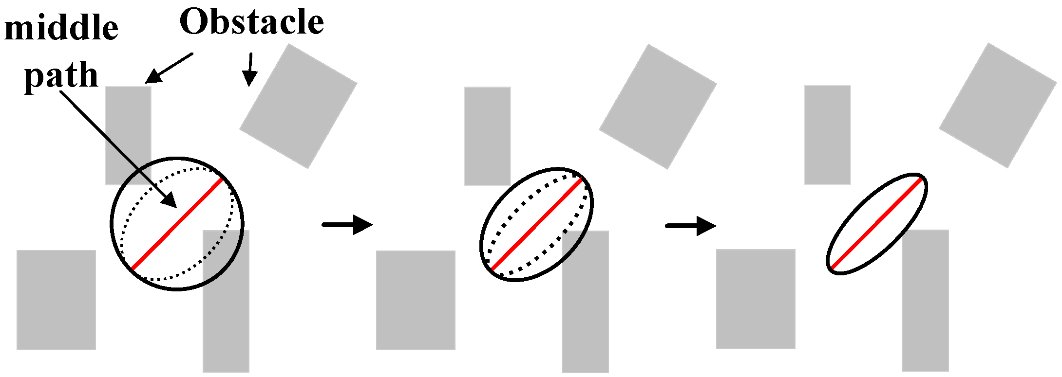
Take a section of the intermediate path determined by any neighboring path points in the whole path as an example. The path is denoted as L. With the path length of L as the diameter, the midpoint for the center of the sphere can be obtained as a sphere. Then, L as a three-dimensional space of a coordinate axis is unchanged, and the contraction of the other two axes ultimately obtains a collision-free maximal ellipsoid. The contraction process in a two-dimensional plane is shown in Figure 3, in which the red line segment is the middle section of the path.
b.
Finding polyhedra
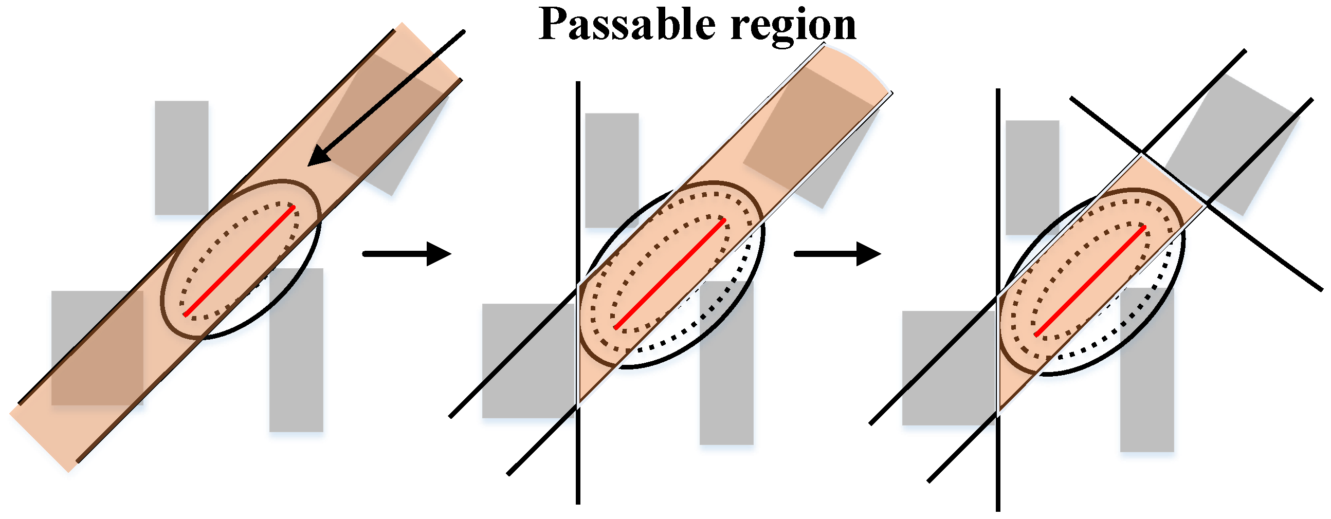
After obtaining the collision-free maximum ellipsoid in the first step, the ellipsoid will have an intersection with the last obstacle. The intersection point of the ellipsoid with this obstacle is used as the tangent point to make the tangent plane of this ellipsoid. Thus, the tangent plane separates the ellipsoid from the obstacle. Then, a half-space without the obstacle can be obtained from this tangent plane. Then, the three axes of the ellipsoid are enlarged in the same proportion until the next obstacle is encountered, and a section separating the next obstacle and a half-space without the next obstacle can be obtained. Cycling this process will eventually result in a convex polyhedron with multiple intersecting facets. The space within the convex polyhedron, i.e., the obstacle-free confined space, is depicted in a two-dimensional form whose process is shown in Figure 4, where the yellow region is the passable region.
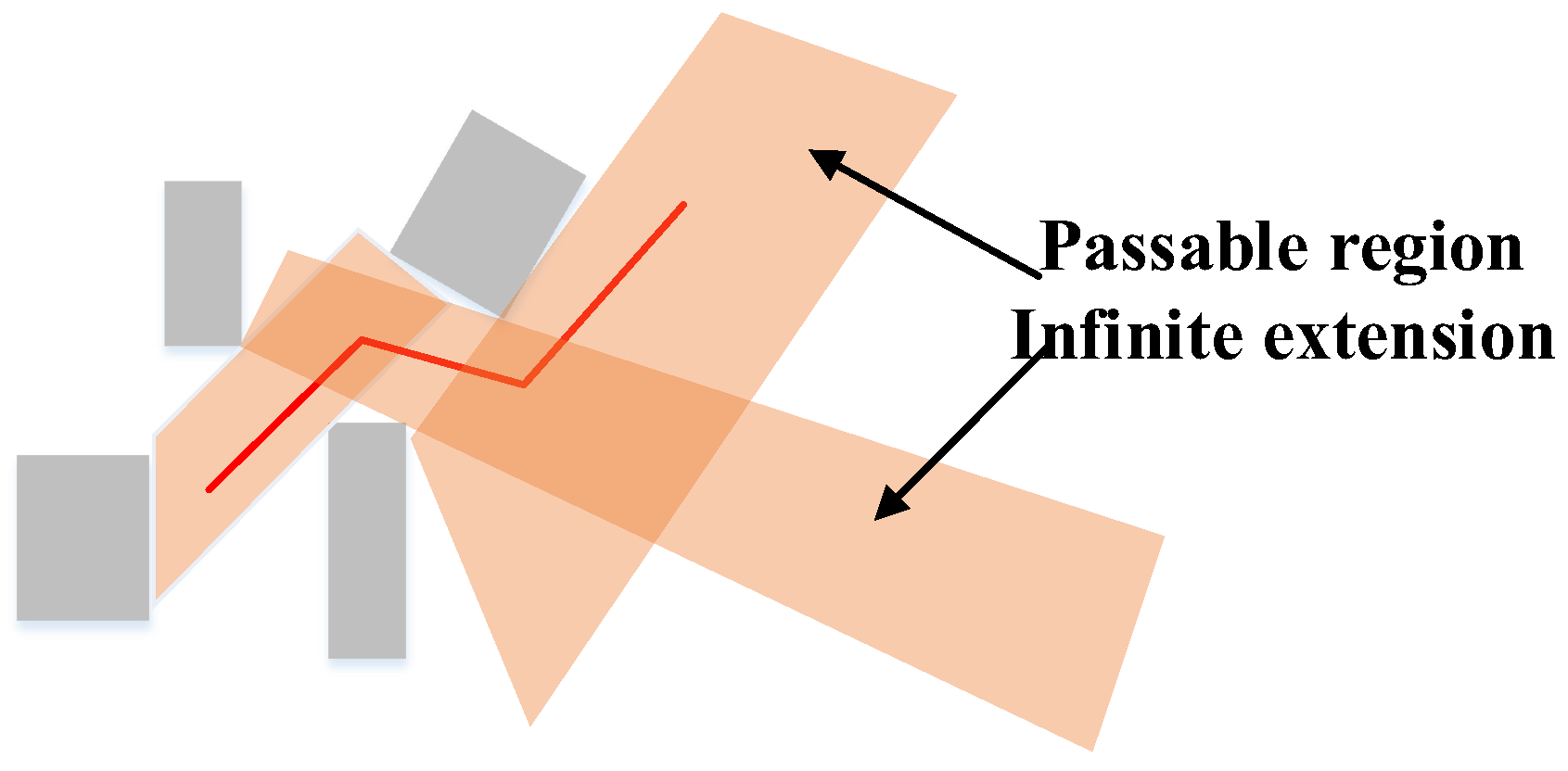
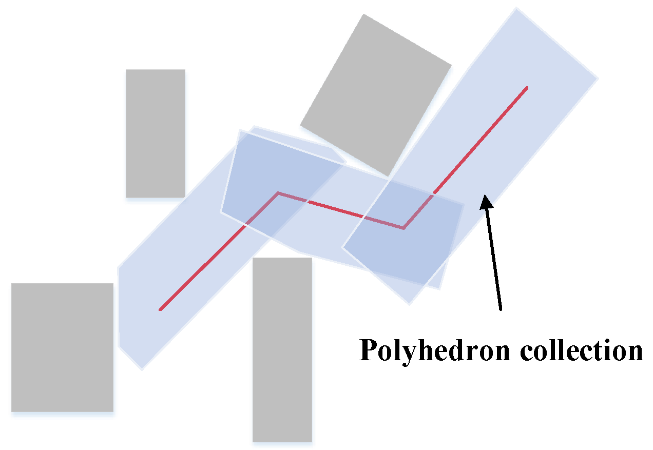
One drawback of this approach is that when a certain plane is missing in order for the intersection of passable spaces to be a closed space and there are no obstacles in this direction, it may require the ellipsoid to expand to a very large size in order to find the point of intersection, or the computation may crash due to the fact that it is never found. The set of polyhedra for multiple paths is shown in Figure 5. This problem will be addressed in the next step.
c.
Setting the bounding box
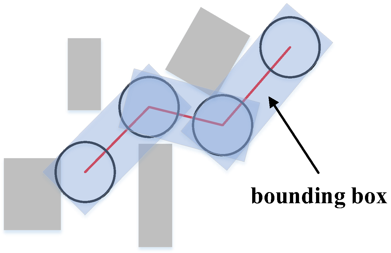
The problem from the previous step can be solved by setting a bounding box. It is equivalent to setting a boundary for the expansion of the ellipsoid. When the boundary is reached in a certain direction before an obstacle is encountered, then the boundary is used as the plane separating the obstacles. This reduces the computation time, and although a lot of passable space may be lost as a result, the fact is that space that is too far from the desired path does not have much practical significance on its own. So, a lot of unnecessary computation is eliminated by setting the bounding box. The effect of setting the bounding box is shown in Figure 6. The length of the short side of the bounding box is the diameter of the circle, the length of the long side is the length of the path plus the diameter of the circle, and the size of the bounding box is determined by defining the diameter of the circle artificially.
A two-dimensional diagram of the polyhedral ensemble after determining the bounding box is shown in Figure 7.
d.
Shrunk
Since it is not possible to treat the robot as a mass in practice, but it is generally necessary to treat the robot as a mass for planning purposes, the resulting convex polyhedral set needs to be shrunk according to the dimensions of the robot. In this way, in the safe corridor formed by the shrunken set of convex polyhedra, the robot can be treated as a mass for planning guaranteed safety. The contracted safe corridor is shown in Figure 8.
If there are a total of M paths from the initial point to the goal point, then the passable region represented by the safety corridor can be expressed as:
F ˜ = i M P i H
where P i H = x R m   A i x _ b i denotes the convex polyhedron obtained after the shrinkage process corresponding to the ith path.

2.2.3. Unconstrained Processing

The most important thing for the robot during the execution of tasks in the underground coal mine environment is safety. In practical applications, most CMRRs usually have a speed of less than 1 m/s. The goal of trajectory planning is that the robot avoids obstacles to reach the target safely, and the MINCO trajectory itself can guarantee the smoothness of the trajectory. Hence, the dynamic constraints G are not given, and the main considerations are the temporal regularity constraint ρ and the safety constraints F ˜ . For problem (11), if we want to deform the MINCO trajectory in time and space to obtain the optimal trajectory, we need to put the cost function, the constraints ρ and F ˜ , into the general optimizer to obtain the MINCO trajectory corresponding to the minimum control cost under the constraints. For the optimizer, the computational cost of optimization with constraints is usually much larger than that of optimization without constraints. Therefore, in order to obtain the optimal trajectory faster by using the spatio-temporal deformation of MINCO, some processing of the constraints ρ and F ˜ are needed to transform the problem into an unconstrained optimization problem for faster solving.
a.
Time regular term constraints
For multiband polynomial curves, the cost function in problem (11) is a function of the polynomial coefficient matrix c and the time vector T, denoted as J c ( c , T ) . The expressions for J c , 𝜕 J c / 𝜕 c , and 𝜕 J c / 𝜕 T are given in [30], and the MINCO trajectory itself belongs to a special subset of multiband polynomials. So, the cost function for this problem can also be written in the following form:
J ( q , T ) = J q ( q , T ) + ρ ( T 1 )
where J q is defined as J q ( q , T ) = J c ( c ( q , T ) , T ) , i.e., the form W ( q , T ) of the cost function on the MINCO trajectory in the previous section. So, J q , 𝜕 J q / 𝜕 q and 𝜕 J q / 𝜕 T are all solvable.
First, for the case in Equation (12), it is defined as follows:
T f = { T R M | T 1 = T Σ , T 0 }
That is, for any 1 i M , the domain of definition of T i is 0 < T i < T Σ . The following mapping transformations are performed on T using variables τ = ( τ 1 , , τ M 1 ) , which can represent all the elements in the space R M 1 :
T i = e τ i 1 + j = 1 M 1 e τ j T Σ , T M = T Σ j = 1 M 1 T j , 1 i < M
where the domain of definition of τ is the whole space of R M 1 . Variation of τ over the whole space of R M 1 can be guaranteed for all cases of T f . So, instead of optimizing the time vector Τ within the constraints T f , the cost function J can be optimized without constraints by τ on R M 1 .
The optimization of the cost function J with respect to the variable τ requires the gradient of J with respect to τ . Divide 𝜕 J q / 𝜕 T into g a R M 1 and g b R , i.e., 𝜕 J q / 𝜕 T = [ g a T , g b ] T . Differentiate Equation (32) and multiply it with 𝜕 J q / 𝜕 T to obtain the gradient of J with respect to the variable τ :
𝜕 J 𝜕 τ = ( g a g a 1 ) e [ τ ] 1 + e [ τ ] 1 ( g a T e [ τ ] g a e [ τ ] 1 ) e [ τ ] ( 1 + e [ τ ] 1 ) 2
where e [ τ ] denotes an element-by-element exponential operation on τ , and 1 denotes a vector with all elements 1.
It is sufficient to use the mapping transformation Τ = e [ τ ] for the case of ρ = ρ s . No new minima are introduced, and no existing minima are eliminated in the optimization process after the mapping from T to τ .
b.
Safety constraints F ˜
F ˜ is the spatial constraint of the safety corridor. A segment of trajectory can be first made to correspond to a subregion. Then, the intermediate path points connecting neighboring trajectories are set in the overlapping region of the two subunits. In this way, the trajectory can be roughly confined to the safe region. If a trajectory is outside the safety region after solving, then a spherical subregion can be artificially set in the middle of the subregion and a path point can be added to the spherical subregion to improve the trajectory, and the solution can be resumed. This is iterated until the entire trajectory is completely inside the safety region. The processing for the trajectories that have appeared outside the safety region is shown in Figure 9.
Based on the above approach, it is necessary to constrain the path points in the overlapping convex polyhedral region of the safety corridor or in the artificial spherical region. The cost function J is also a function of the path point vector q . So, the problem becomes optimizing the cost function J when the path point vectors q are under the safety constraints. The problem is converted to an unconstrained optimization problem before solving it, and the constraints to be dealt with are spherical constraints and polyhedral constraints.
  • Spherical constraints
A spherical constraint has q P B R m for any intermediate path point, where P B is a closed sphere. Its radius is r and the center point is o . Then, it can be expressed as:
P B = x R m   x o 2 r
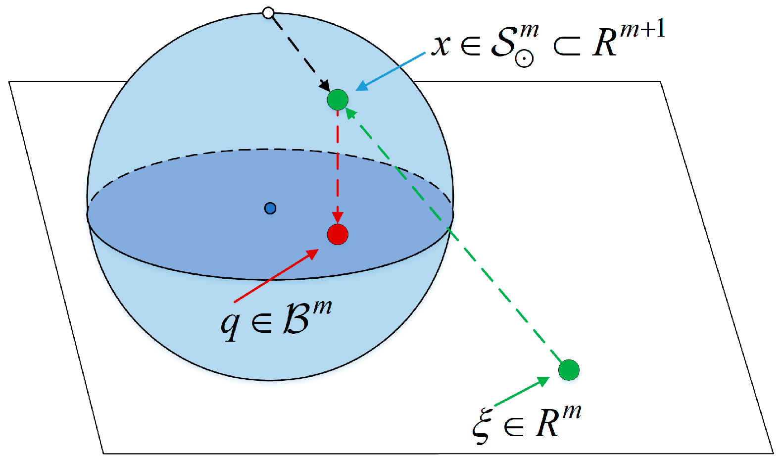
The transformation can be used to map the whole space R m into P B to obtain an unconstrained optimization variable in space R m . The whole process is illustrated in two-dimensional and three-dimensional forms and is shown in Figure 10.
Map the entire space R m to a unit sphere in space R m + 1 without the North Pole as follows:
S m = { x R m + 1 | x 2 = 1 , x m + 1 < 1 }
Denote this mapping as f s :
f s ( x ) = ( 2 x T , x T x 1 ) T x T x + 1 S m , x R m
The unit sphere S m defined in space R m + 1 is then projected into space R m to obtain the unit sphere B m defined in space R m :
B m = { x R m | x 2 1 }
Denote this mapping as f o :
f o ( x ) = ( x 1 , , x m ) B m , x S m
Then, all positions except the midpoint in B m can correspond to two positions on the sphere S m . Finally, a linear mapping is added to change the radius so that B m can map to P B . By combining the mapping f s , f o , and the linear mapping, a composite mapping f B from the whole space R m to the sphere P B in space R m can be obtained:
f B = o + 2 r x x T x + 1 P B , x R m
Represent the variables in Equation (39) as a new variable ξ . For arbitrary ξ R m , q mapped by f B always results in a spherical constraint. Thus, the cost function can be optimized in space R m for unconstrained variables ξ instead of optimizing q in the constraints P B . However, the optimization on ξ requires a gradient 𝜕 J / 𝜕 ξ . If we denote the ith element of 𝜕 J / 𝜕 q i by g i , then the gradient of J to ξ i (the ith element in ξ ) can be obtained by computing the differential of the mapping f B :
𝜕 J 𝜕 ξ i = 2 r i g i ξ i T ξ i + 1 4 r i ( ξ i T g i ) ξ i ( ξ i T ξ i + 1 ) 2
Compute 𝜕 J / 𝜕 ξ i ( 1 i M ) to obtain the 𝜕 J / 𝜕 ξ . Then, the constrained optimization problem becomes an unconstrained optimization problem over the variable ξ .
  • Convex polyhedral constraints
The set of convex polyhedra is denoted as P H , which can be expressed as:
P H = { x R m | A x _ b }
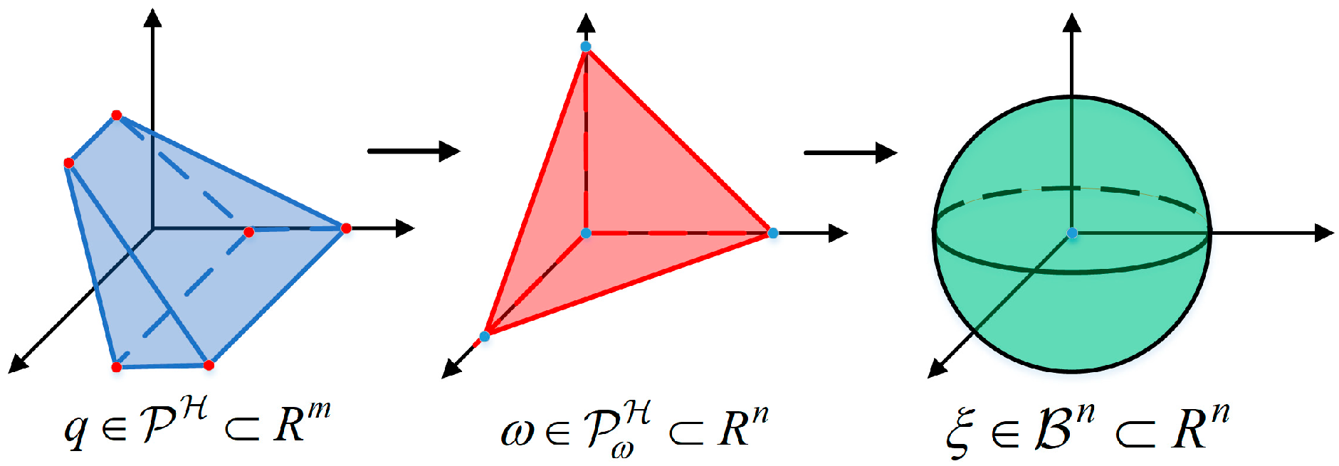
For a general convex polyhedron, all points q in the interior can be represented by their vertex coordinates. When the dimension is low and the vertex coordinates are easy to obtain, then all points q in the convex polyhedron constraint can be parameterized by their vertex coordinates. If the convex polyhedron in P H has n + 1 vertex, denote its vertex by ( v 0 , , v n ) , where v i R m . To visualize the convex polyhedron vertices in terms of q , let v ¯ i = v i v 0 and V ¯ = ( v ¯ 1 , , v ¯ n ) ; then, the relationship between q with the vertices can be expressed as:
q = v 0 + V ¯ ω
where ω = ( ω 1 , , ω n ) T R n . It is equivalent to representing a convex polyhedron with the origin v 0 and the vectors between v 0 and the other vertices as edges, denoted as P ω H :
P ω H = { ω R n | ω _ 0 , ω 1 1 }
All points q in the original polyhedron can be expressed in coordinates ω . The transformation between P ω H and P H is equivalent in (42). By using the square transformation ω = [ x ] 2 , a simple polyhedron P ω H can be converted into a unit ball B n :
B n = { x R n | x 2 1 }
The treatment of the ball constraint has already been discussed, so after the transformation in (42), the square transformation ω = [ x ] 2 , and the composite transformation in f B in formula (39), the transformation that maps the constraint P H to the whole space R n can be obtained, denoted as f H :
f H = v 0 + 4 V ¯ [ x ] 2 ( x T x + 1 ) 2 P H , x R n
The processing of the convex polyhedral constraints is shown in Figure 11:
Furthermore, the new variables introduced for f H are denoted as ξ . Then, any ξ R n can correspond to a q P H , and ξ in the entire space R n can fill the entire convex polyhedra P H by transformations. Denote g i as the ith element of 𝜕 J / 𝜕 q , i.e., 𝜕 J / 𝜕 q i ; then, the ith element of the gradient of the cost function with respect to the new variable ξ is:
𝜕 J 𝜕 ξ i = 8 ξ i V ¯ T g i ( ξ i T ξ i + 1 ) 2 16 g i T V ¯ [ ξ i ] 2 ( ξ i T ξ i + 1 ) 3
The transformation process does not introduce new minima, nor does it eliminate existing minima. Thus, for the spatial safety constraints q in F ˜ , it can be unconstrained by proxy variables ξ .

2.2.4. MINCO Trajectory-Based Planning Approach

The cost function for the spatio-temporal deformation of a MINCO trajectory can be written as J ( q ( ξ ) , T ( τ ) ) . The optimization of the cost J to the variables ξ and τ is an unconstrained optimization problem. By handing it over to a general-purpose optimizer, we can quickly solve ξ and τ at the minimum cost. The path point vectors q and time vectors T corresponding to the minimum cost are then obtained by mapping. Thus, with the customized boundary conditions q and T , a feasible trajectory that fits the robot kinematics model with optimal control cost under the constraints of the underground coal mine environment can be obtained.
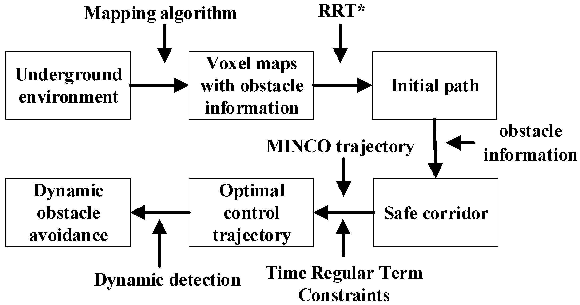
After the above analysis, the overall process of the trajectory planning method is:
(1) Firstly, process the underground coal mine environment constraints to obtain the voxel map containing obstacle information;
(2) Quickly obtain a good path on the voxel map with the RRT* algorithm;
(3) Generate a safe corridor from the path and obstacle information obtained at the front end;
(4) Apply MINCO trajectories and their spatio-temporal deformations to generate optimal trajectories under safe corridor constraints and temporal regularity term constraints;
(5) After obtaining the optimal trajectory, refresh the map at certain time intervals and inflate the obstacles appropriately. Perform collision detection on the trajectory after obtaining the new voxel map. If the trajectory is not safe enough or new obstacles appear on the trajectory, then repeat the above process to replan for dynamic obstacle avoidance.
The flowchart of the MINCO trajectory planning method is shown in Figure 12:

3. MPC-Based Trajectory Tracking for Mobile Robots

3.1. Modeling of Robot Kinematics

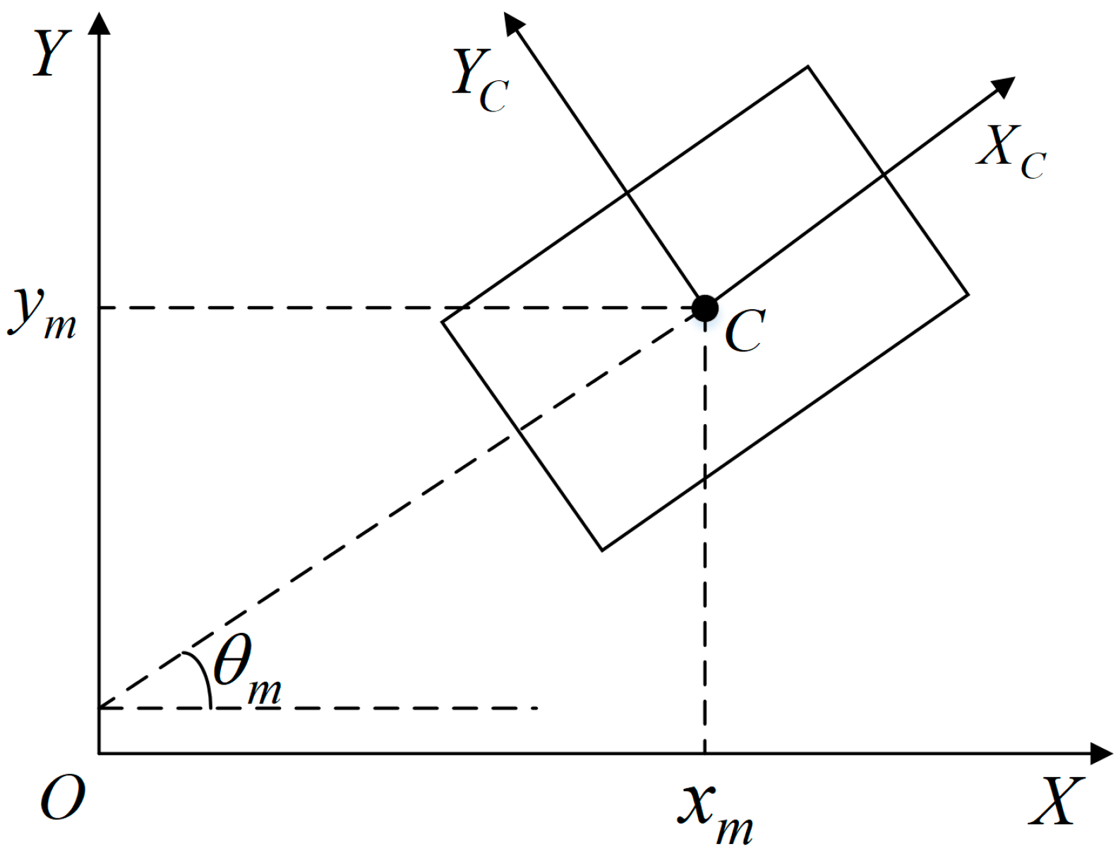
The design of the MPC controller system model is based on the kinematic model of the underground CMRRs. Assuming that no relative sliding between the track and the ground occurs, the robot kinematic model can be built as shown in Figure 13.
The point C is the center point of the robot, with coordinates ( x m , y m ) , and θ m is the heading angle of the robot. X C and Y C are the coordinate axes of the robot’s forward direction and its vertical direction, respectively. The state information of the robot at any moment is represented by P m ( x m , y m , θ m ) . Then, the robot’s kinematic equations can be expressed as follows:
x ˙ m = v m cos θ m y ˙ m = v m sin θ m θ ˙ m = ω m
where v m denotes the linear velocity of the robot in the axis direction X C . ω m denotes the angular velocity of the robot. x m and y m denote the velocities in the X axes and Y axes of the world coordinate system, respectively. If the state vector of the robot is denoted by X m ( x m , y m , θ m ) T , the kinematic equations of Equation (47) can be written in the following matrix form:
X ˙ = x ˙ m y ˙ m θ ˙ m = cos θ m 0 sin θ m 0 0 1 v m ω m = f ( X m , u m )
where X ˙ is the derivative of the state quantity with respect to time t ; u = ( v m , θ m ) T is a function of time t , which is the control quantity of the robot.
For the tracked CMRR, it is necessary to convert the control quantity u into the speed of the left and right tracks in order to finally control the robot’s motion. The relationship between the robot’s linear velocity, angular velocity, and the left and right track velocities during differential motion is as follows:
v m ω m = 1 2 1 2 1 2 L 1 2 L v L v R
where v L and v R are the left and right track speeds, respectively.
The differential flatness of the robot kinematic model is further verified. The function z = ( x m , y m ) T about time t is chosen as the flat output; then, the state variables of the robot can be expressed as:
x m y m θ m = x m y m arctan ( y ˙ m x ˙ m )
The control variables of the robot can be expressed as:
v m ω m = x ˙ m 2 + y ˙ m 2 y ¨ m x ˙ m y ˙ m x ¨ m ( x ˙ m + y ˙ m ) 2
Thus, both the state and control quantities of the system can be determined by the flat output and its finite dimensional derivatives, proving the differential flatness of the robot kinematic model.

3.2. MPC-Based Trajectory Tracking Control for Mobile Robots

3.2.1. Construction of Predictive Models

P r ( x r , y r , θ r ) is the target pose of the robot, where ( x r , y r ) and θ r are the target position and target heading angle, respectively. Then, the target trajectory can be written in the following form according to Equation (48):
X ˙ r = x ˙ r y ˙ r θ ˙ r = cos θ r 0 sin θ r 0 0 1 v r ω r = f ( X r , u r )
Equation (52) is a nonlinear equation. It is linearized and approximated for ease of computation. A first-order Taylor expansion and omission of higher-order terms at the target position is shown as:
X ˙ = f ( X r , u r ) + f X , r ( X X r ) + f u , r ( u u r )
where f X , r is the Jacobi matrix of f with respect to X . f u , r is the Jacobi matrix of f with respect to u :
f X , r = 0 0 v r sin θ r 0 0 v r cos θ r 0 0 0 , f u , r = cos θ r 0 sin θ r 0 0 1
Denoting X ˙ ¯ , A , B , X ¯ , and u ¯ as X ˙ X ˙ r , f X , r , f u , r , X X r , u u r , respectively, is shown as:
X ˙ ¯ = A X ¯ + B u ¯
where X ¯ denotes the error between the actual robot position and the target position. u ¯ denotes the error between the actual control quantity and the target control quantity. The system error model shown in Equation (55) can be obtained by discretizing it by the forward difference method:
X ˙ ¯ = X ¯ ( k + 1 ) X ¯ ( k ) T = A ( k ) X ¯ ( k ) + B ( k ) u ¯ ( k )
where T is a control cycle and k is the sampling moment. Equation (56) can be changed into:
X ¯ ( k + 1 ) = ( I + T A ( k ) ) X ¯ ( k ) + T B ( k ) u ¯ ( k )
Set A ¯ ( k ) = I + T A ( k ) , B ¯ ( k ) = T B ( k ) , then:
X ¯ ( k + 1 ) = A ¯ ( k ) X ¯ ( k ) + B ¯ ( k ) u ¯ ( k )
Equation (58) is the MPC prediction model, where A ¯ ( k ) and B ¯ ( k ) can expand as:
A ¯ ( k ) = 1 0 v r ( k ) sin θ r ( k ) T 0 1 v r ( k ) cos θ r ( k ) T 0 0 1 , B ¯ ( k ) = cos θ r ( k ) T 0 sin θ r ( k ) T 0 0 T

3.2.2. Design of Objective Function and Constraints

The goal of the MPC trajectory tracking controller is to have as small an error as possible in the robot’s position and the desired trajectory to realize the tracking of the target trajectory, and at the same time, to have as small an error as possible in the control volume to ensure that the speed change is as smooth as possible. Therefore, the cost function at time k can be designed in the following form:
J ( k ) = j = 1 N X ¯ ( k + j | k ) T Q X ¯ ( k + j | k ) + u ¯ ( k + j 1 | k ) T R u ¯ ( k + j 1 | k )
where N is the predicted time domain of the MPC for the system; Q and R are the weight matrices of the position error and the weight matrix of the control volume error, and both are positive definite diagonal matrices. X ¯ ( k + j | k ) and X ¯ ( k + j | k ) T Q X ¯ ( k + j | k ) denote the pose error and the pose error cost of the j step predicted at the time k. u ¯ ( k + j 1 | k ) and u ¯ ( k + j 1 | k ) T R u ¯ ( k + j 1 | k ) denote the control error and the control error cost of the j step predicted at the time k.
In the prediction time domain of the time k , the predicted future N step robot position error and control volume error can be written in the matrix form as:
X ˜ ( k ) = X ¯ ( k + 1 | k ) X ¯ ( k + 2 | k ) X ¯ ( k + N | k ) , u ˜ ( k ) = u ¯ ( k | k ) u ¯ ( k + 1 | k ) u ¯ ( k + N 1 | k )
where X ˜ ( k ) is the attitude error matrix and u ˜ ( k ) is the control volume error matrix. Thus, the cost function can be written as:
J ( k ) = X ˜ ( k ) T Q ¯ X ˜ ( k ) + u ˜ ( k ) T R ¯ u ˜ ( k )
where:
Q ¯ = Q 0 0 0 Q 0 0 0 Q , R ¯ = R 0 0 0 R 0 0 0 R
Assume that A ¯ ( k ) and B ¯ ( k ) are constant at a fixed value during a control cycle, denoted as A ¯ , B ¯ . The relationship between the position matrix and the control volume matrix is:
X ˜ ( k ) = A ˜ X ¯ ( k ) + B ˜ u ˜ ( k )
where X ¯ is the initial condition of the moment k , i.e., the current state deviation of the robot. A ˜ and B ˜ can be expressed as follows:
A ˜ = A ¯ A ¯ 2 A ¯ N , B ˜ = B ¯ 0 0 A ¯ B ¯ B ¯ 0 A ¯ N 1 B ¯ A ¯ N 2 B ¯ B ¯
Bringing Equation (64) into (62) gives the cost function as:
J ( k ) = 1 2 u ˜ ( k ) T H u ˜ ( k ) + C T u ˜ ( k ) + D
where:
H = 2 ( B ˜ T Q ¯ B ˜ + R ¯ ) C = 2 ( B ˜ T Q ¯ A ˜ T X ¯ ( k ) ) D = X ¯ ( k ) T A ˜ T Q ¯ A ˜ X ¯ ( k )
D is only related to the current actual state error, which is a known quantity. Equation (66) is the standard quadratic programming form on the u ˜ ( k ) .
In the real system, the control quantity will be subject to the actual physical limitations and the existence of upper and lower limits, or the user will want to set the control quantity that must be within a range. So, it is necessary to give some constraints on the control quantity in the optimization solution process, which can be expressed in the following form:
u ˜ min u ˜ ( k ) u ˜ max u min u ( k ) u max
where u ( k ) and u ˜ ( k ) are the control volume matrix and the control volume error matrix, respectively. The optimal control quantity is then obtained by solving this quadratic programming problem with constraints.

4. Experiments on Trajectory Planning and Tracking of CMRRs

4.1. Experiments on Trajectory Planning of CMRRs

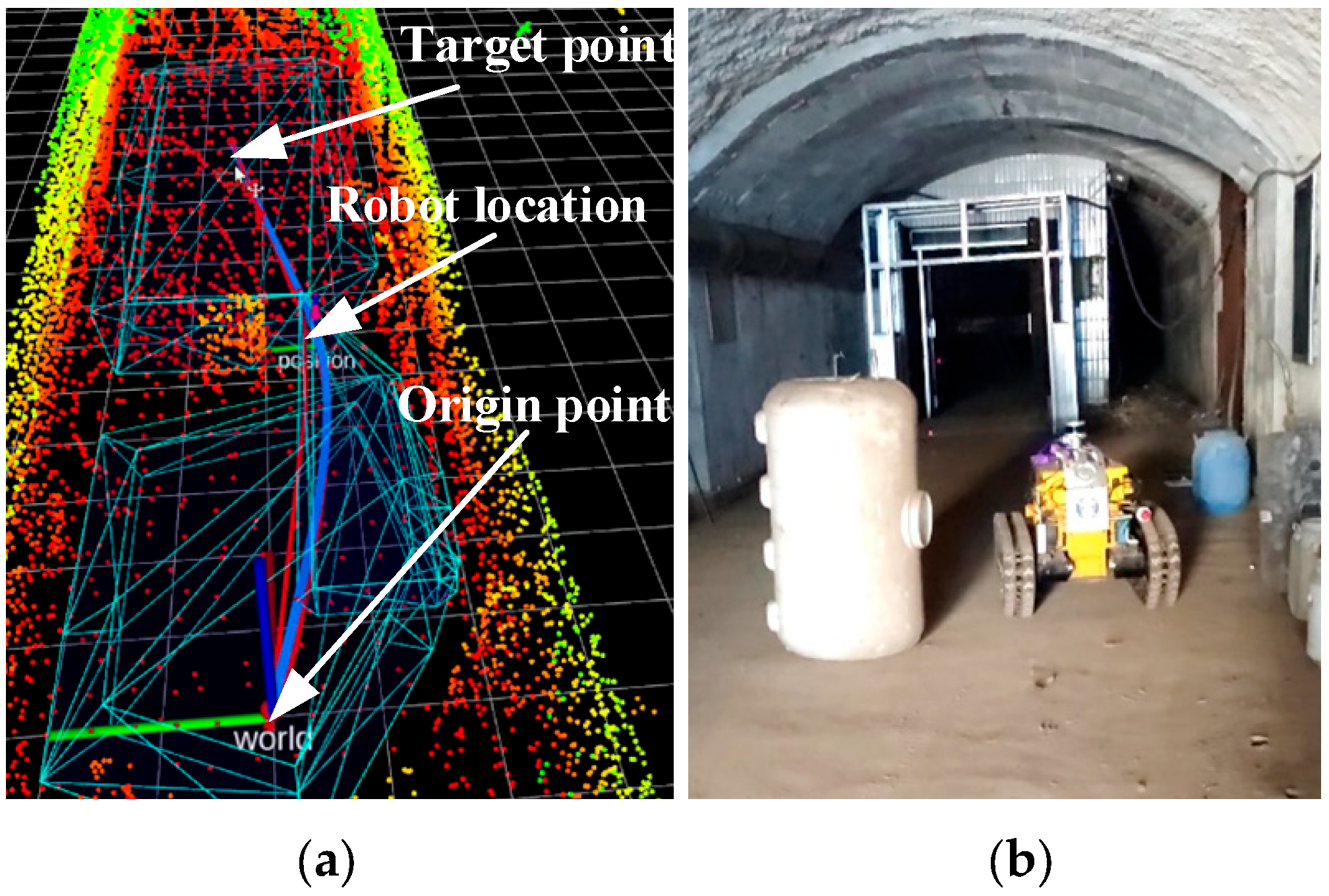
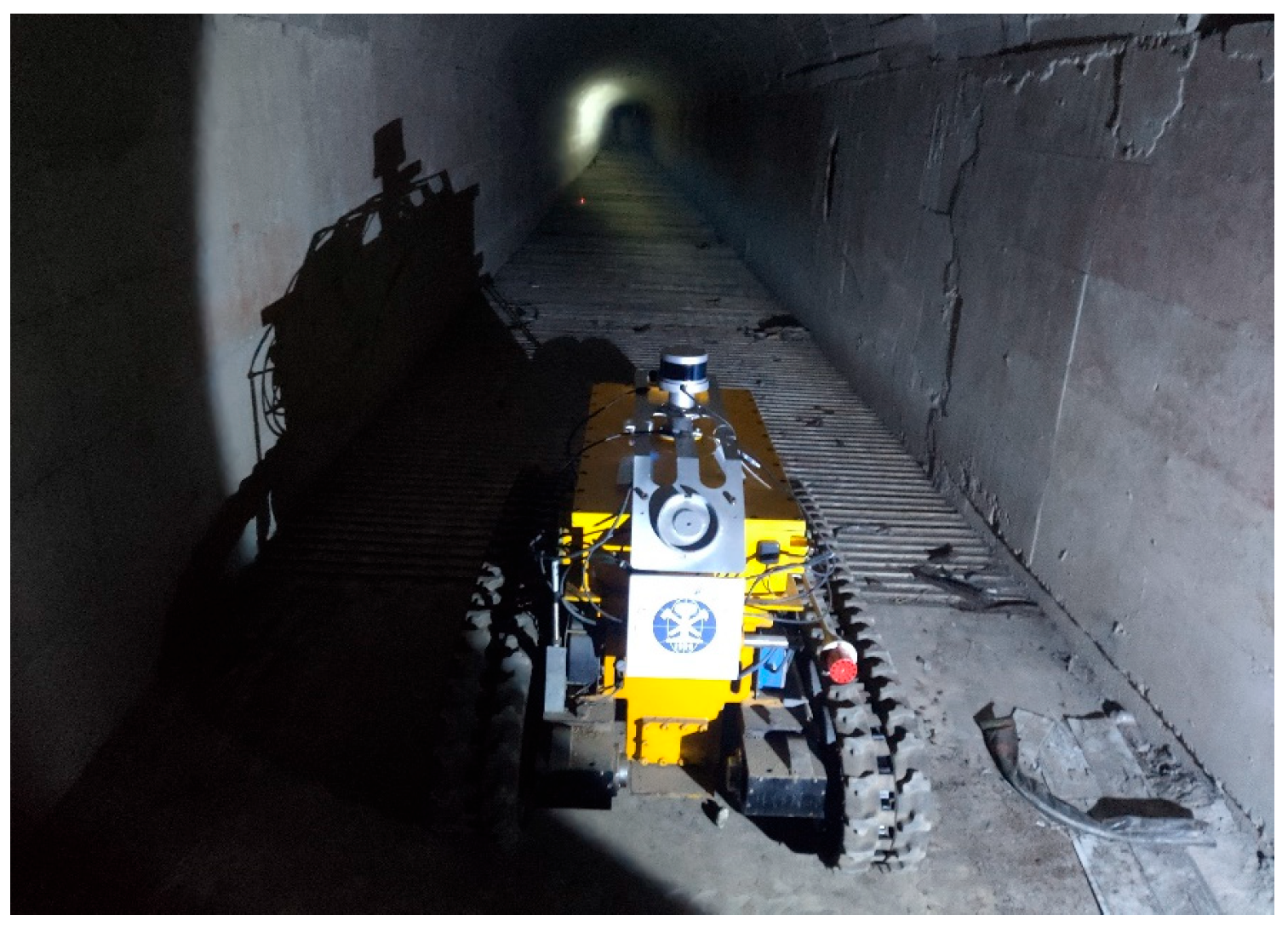
In order to verify the practicality of the MINCO trajectory planning method, a multiscenario experiment was conducted in a simulated tunnel in the Gas and Coal Dust Explosion Laboratory of China University of Mining and Technology. The mobile robot platform and experimental environment used for the experiments are shown in Figure 14. The mobile robot is realized by the differential speed control of the left and right tracks to realize the robot’s motion.
The simulated tunnel is extremely similar to a real coal mine laneway in terms of structure, walls, and other features. In order to simulate the obstacles in a manner that resembles a real underground environment, different experimental scenarios are designed by setting static obstacles, such as buckets, and dynamic obstacles of characters in the simulated tunnel to conduct robot-trajectory-planning and -tracking experiments. The experiments of a single obstacle scenario, multiple obstacle scenario, dynamic obstacle scenario, and right-angle turn scenario were carried out sequentially to examine the practicality and robustness of the robot trajectory planning algorithm.
We conducted experiments to fully simulate an underground tunnel environment using a coal mine rescue robotic platform carrying a special sensor configuration with two Velodyne VLP-16 LiDARs. One of the horizontally deployed LiDARs was used to execute the LOAM [31] algorithm, which was used to further construct voxel maps and in turn execute the MINCO trajectory-planning methods. The tracking module used by the robot is the MPC controller from the previous section. The localization and mapping algorithm used by the robot is LOAM, which can output the mapping results and its own position information in real time.

4.1.1. Static Scene Planning Experiment

a.
Single Obstacle Scene Planning Experiment
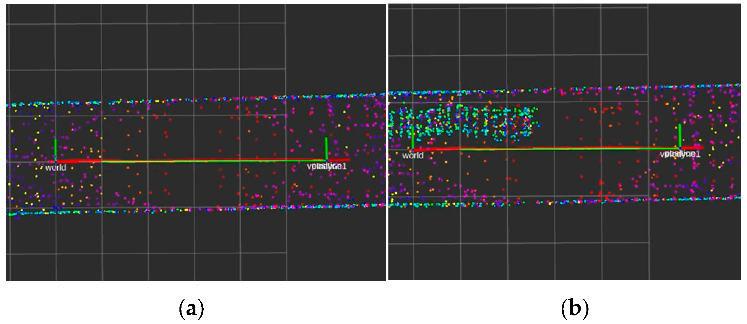
The first is a simple single obstacle scenario. A bucket is artificially set as a static obstacle at about 4.5 m in front of the robot start point. As shown in Figure 15a, the target point is set about 12 m in front of the start point to examine the robot’s trajectory planning effect. Figure 15b shows the corresponding RVIZ 3D point cloud, in which “world” represents the world coordinate, the red axis is the X-axis, the green axis is the Y-axis, the blue axis is the Z-axis, and the coordinate “position” indicates the robot position. The initial robot position coincides with the world coordinates.
Compare the MINCO trajectory-based planning method with the Fast-Planner algorithm [32]. In the experiment, the robot was remotely controlled to the same initial point position; the two algorithms were run separately. Then, the same target point was given for comparison. The experimental results of the MINCO trajectory method are shown in Figure 16. The blue curve is the target trajectory planned by the algorithm, and the light-blue polyhedron is the safety corridor. Figure 16a shows the planning results, and Figure 16b shows the actual positional relationship when the robot moves next to an obstacle.
The experimental results of the Fast-Planner planning algorithm are shown in Figure 17. The red curve is the target trajectory planned by the algorithm. Figure 17a shows the initial planning results, and Figure 17b shows the results after the algorithm replanning. Replanning is performed with the current position of the robot as the starting point, and the target point remains unchanged. Figure 17c,d show the 3D point cloud map and the actual position relationship when the robot moves next to an obstacle, respectively.
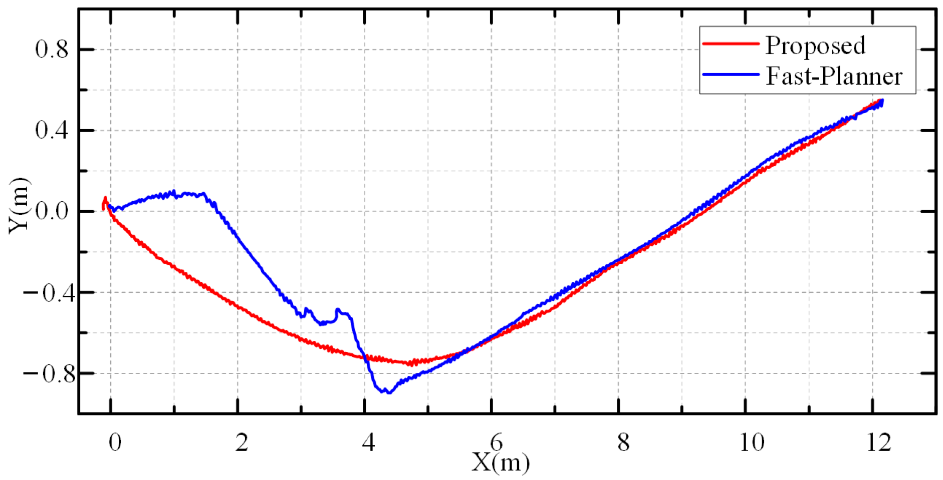
The MINCO trajectory method performs only one planning in the initial stage of the robot movement, and the planning time is 0.029 s. The trajectory is sampled at the X-axis interval of 0.05 m to obtain the sampled trajectory points (all the points below are sampled at the X-axis interval of 0.05 if not pointed out), and the length of the planned trajectory is calculated to be 12.54 m. The Fast-Planner algorithm performs three planning times in the whole process, with a total time of 0.034s, and the length of the robot trajectory was 12.75 m.
The localization information in the LOAM algorithm was used to obtain the two real running trajectories of the robot in the laneway, respectively. The algorithm trajectory comparison is shown in Figure 18. It can be seen that compared with the Fast-Planner algorithm, in the case of single obstacle planning, the MINCO trajectory method is better than the Fast-Planner algorithm both in the planning time, trajectory length, and in the trajectory smoothing, which is more suitable for underground mobile robots. The reason is because the algorithm in this paper plans within the safety corridor, the safety threshold is large enough in this simple scenario, and only one planning is performed, so the total planning time is less. Because it is based on MINCO trajectory optimization on flat space, which conforms to the robot kinematic model while minimizing the control cost, the trajectory is smoother and the trajectory length is shorter.
b.
Multiobstacle Scene Planning Experiment
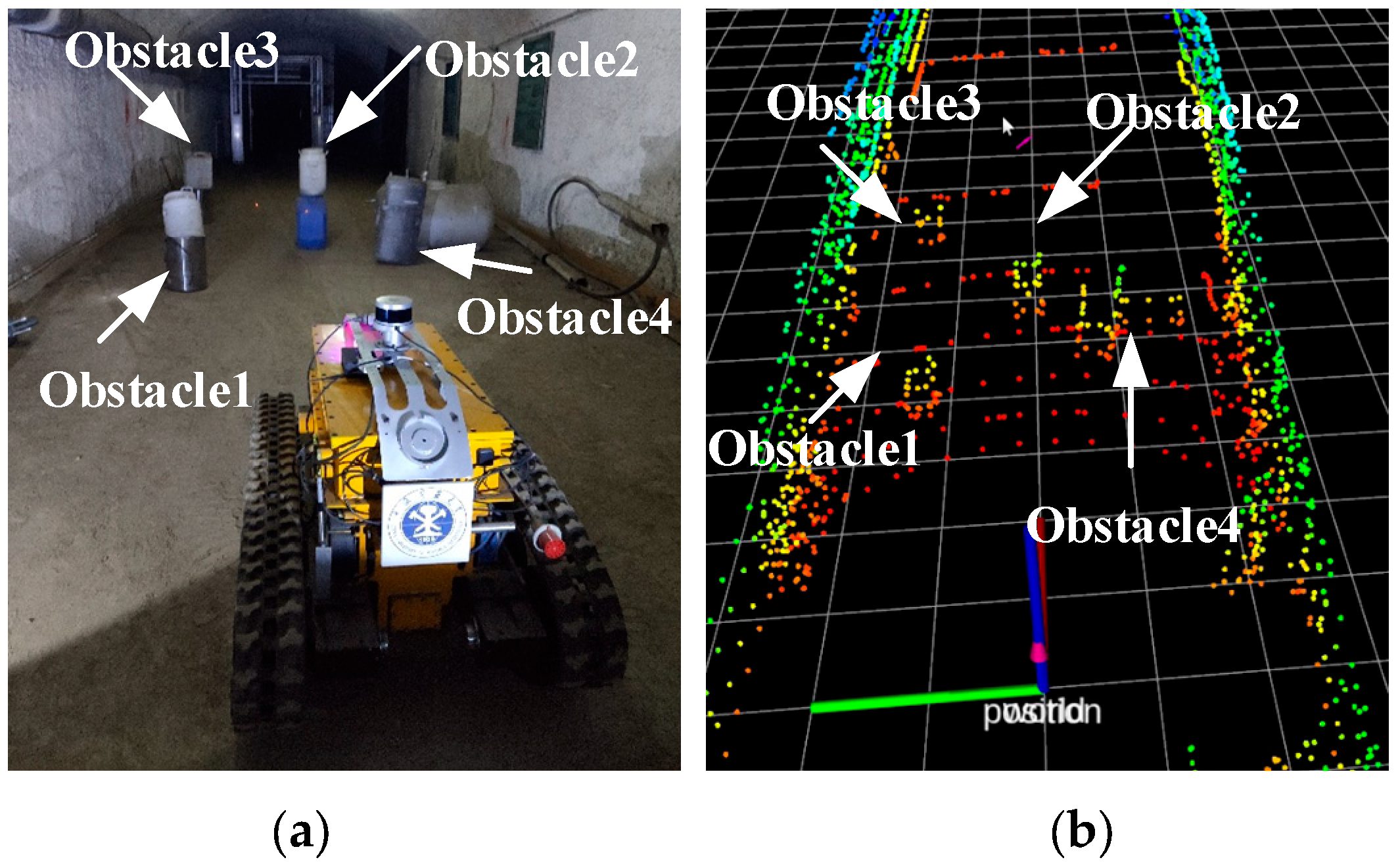
The relationship between obstacles and the initial position of the robot in the multiobstacle scene is shown in Figure 19, where obstacle 2 is about 5 m in front of the robot. The X-axis and Y-axis distances between obstacle 1 and obstacle 2 are about 1.3 m and 0.9 m. The X-axis and Y-axis distances between obstacle 3 and obstacle 2 are about 1.4 m and 1.1 m. Obstacle 4 completely blocks the road on the right side, and obstacle 1 and obstacle 3 are at a small distance from the left laneway wall, so the robot cannot pass through them either. The planning experiment was conducted by setting the target point about 10.6 m in front of the robot. The ideal situation is that the robot passes through the middle of the obstacles and reaches the end point without hitting the obstacles.
The experiments also compare the planning of the MINCO trajectory method with the Fast-Planner algorithm. The experimental results of the MINCO trajectory method are shown in Figure 20. Figure 20a shows the initial planning result given by the algorithm, Figure 20b shows the final planning result of the algorithm and the point cloud map of the robot moving into the obstacle interval, and Figure 20c,d show the map of the actual position of the robot entering the obstacle interval and leaving the obstacle interval, respectively.
The experimental results of the Fast-Planner planning algorithm are shown in Figure 21. Figure 21a shows the initial planning result given by the algorithm. Obviously, this trajectory does not avoid the obstacles. Figure 21b shows the final planning result of the algorithm and the point cloud of the robot movement regarding the obstacle interval. The final planning is completed only when the robot moves close to the obstacle, where the red curve without points is the actual trajectory of the robot. Figure 21c,d show the actual position maps of the robot entering the obstacle interval and leaving the obstacle interval, respectively.
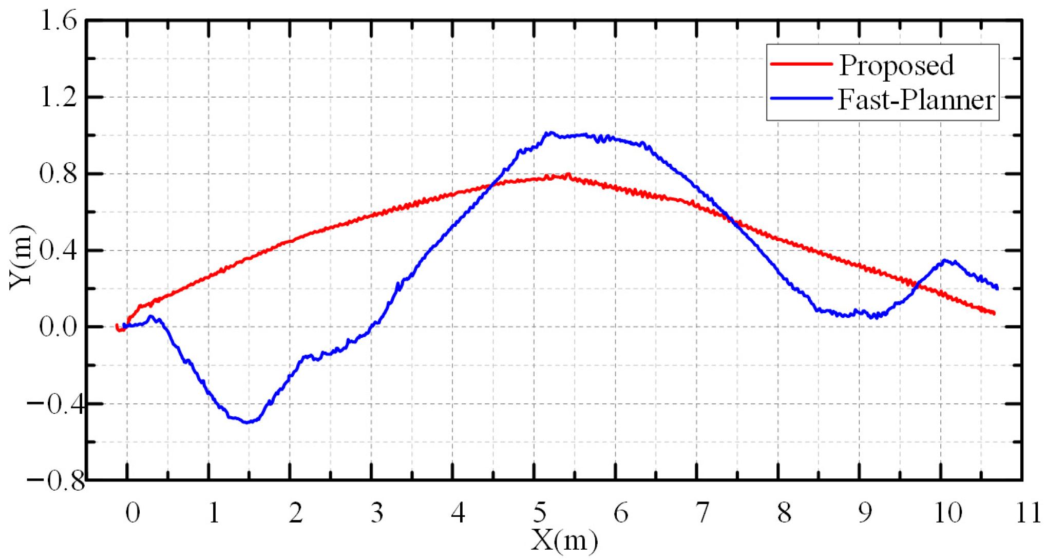
The final trajectories of the MINCO trajectory method and the Fast-Planner algorithm are shown in Figure 22. The MINCO trajectory method plans a total of eight times during the robot movement, with a total planning time of 0.18 s, and the length of the robot movement trajectory is 11.04 m. The Fast-Planner algorithm performs a total of 38 planning times during the whole process, with a total time of 0.375 s, and the length of the robot motion trajectory is 11.71 m.
From the above data as well as the trajectory comparison graphs, it can be seen that the MINCO trajectory method is better than the Fast-Planner algorithm in a number of indexes in the case of multiple static obstacles, and is more suitable for CMRRs.
Next, some phenomena in the experiment are analyzed. Since the length and width of the robot used in the experiment are about 1.2 m and 0.8 m, and the X-axis and Y-axis distances between obstacle 1 and obstacle 2 are only 1.3 m and 0.9 m, the safety thresholds are very small. So, both algorithms plan several times to adjust them. The Fast-Planner algorithm, because the front-end search does not involve the environment information, needs several adjustments to complete the whole trajectory planning task, resulting in a costly trajectory with multiple turns. The MINCO trajectory method completes the safe corridor generation after the front-end search, and then carries out the generation of the optimal trajectory within the safe corridor, so the whole trajectory planning process avoids obstacles, and therefore, a better result can be obtained in the first planning. Because the safety threshold is too small, several replannings are carried out when judging whether the trajectory is safe or not, but the number of times is much smaller than the Fast-Planner algorithm.
c.
Planning experiments in right-angle turn scenarios
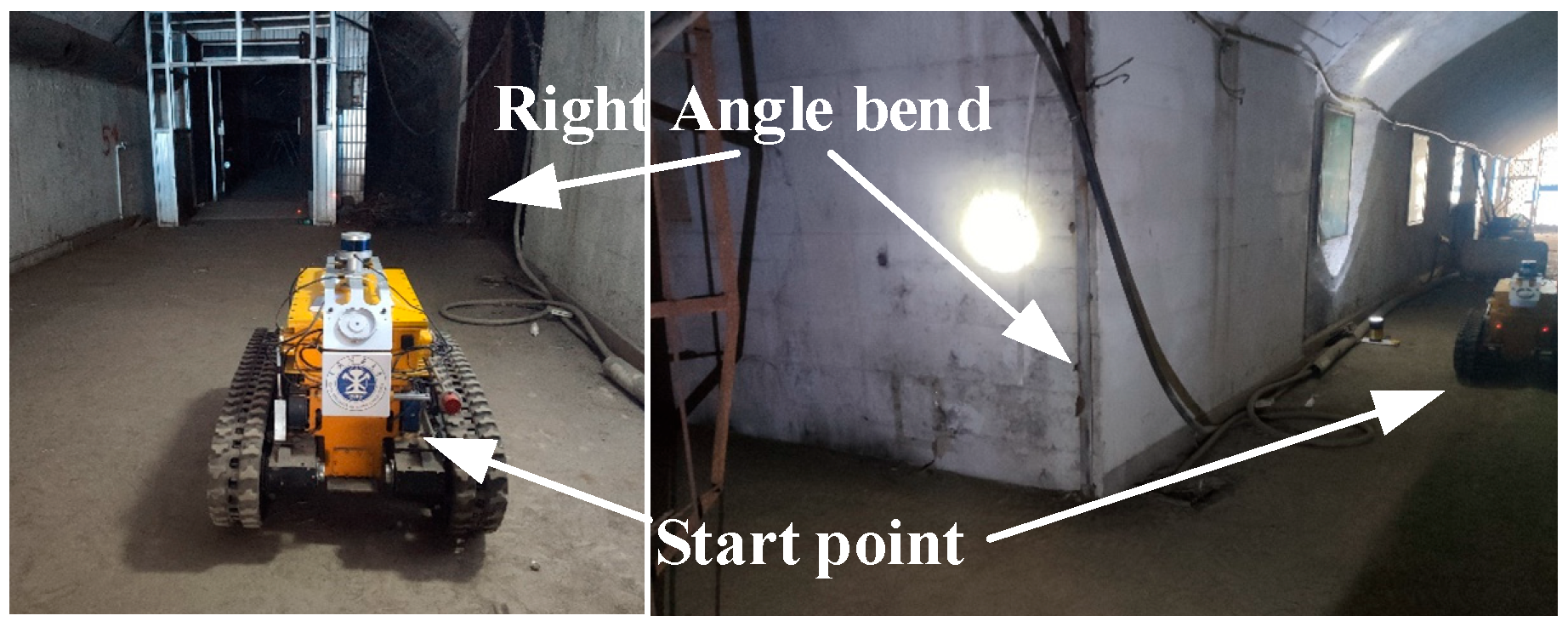
The real underground environment has complex intersecting lanes, and the lanes often intersect each other in the form of close to a right-angle. So, a right-angle turn scenario planning experiment was designed for testing. The experimental scene is shown in Figure 23, and the target point is set at about 4 m past the right-angle turn, and the X-axis and Y-axis relative to the initial position of the robot are 6 m and −6 m, respectively.
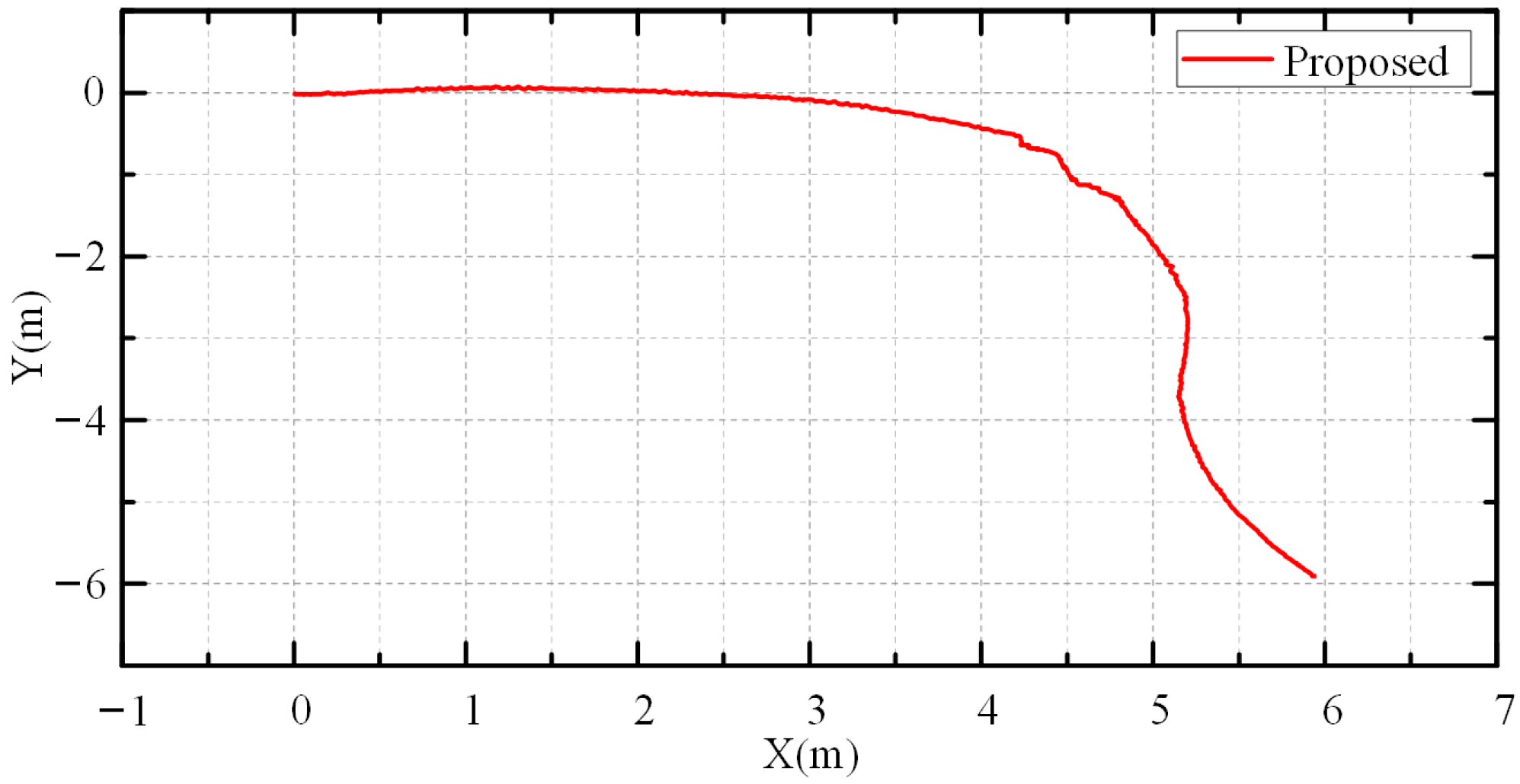
The experimental results of the MINCO trajectory method are shown in Figure 24. Figure 24a shows the first planning result given by the algorithm, and Figure 24b shows the result of replanning when the robot enters the bend. Figure 24c shows the positional attitude of the robot as it enters the turn. Figure 24d shows the positional attitude of the robot when it exits the turn.
The experimental results of the Fast-Planner planning algorithm are shown in Figure 25. In the right-angle turn scenario, the Fast-Planner algorithm cannot plan a reasonable trajectory.
The robot motion trajectory of the MINCO trajectory method is shown in Figure 26. In this scenario, a total of six plannings were carried out during the robot motion, with a total planning time of 0.428 s. The length of the robot motion trajectory was 11.63 m. The Fast-Planner algorithm fails to plan in this scenario. Since there is no environmental input to the front-end search of the Fast-Planner method, the algorithm relies mainly on the continuous replanning and optimization of the back-end for trajectory planning. However, the back-end adjustment is based on the front-end search results. The distance from the path point to the passable place of this front-end search result is much larger than the previous scenarios, which leads to the algorithm’s inability to find a safe trajectory, and it ultimately fails to complete the planning.

4.1.2. Planning Experiments in Dynamic Scenarios

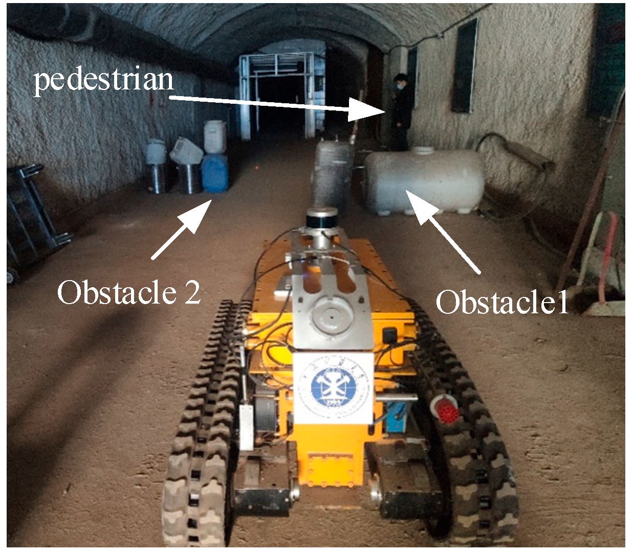
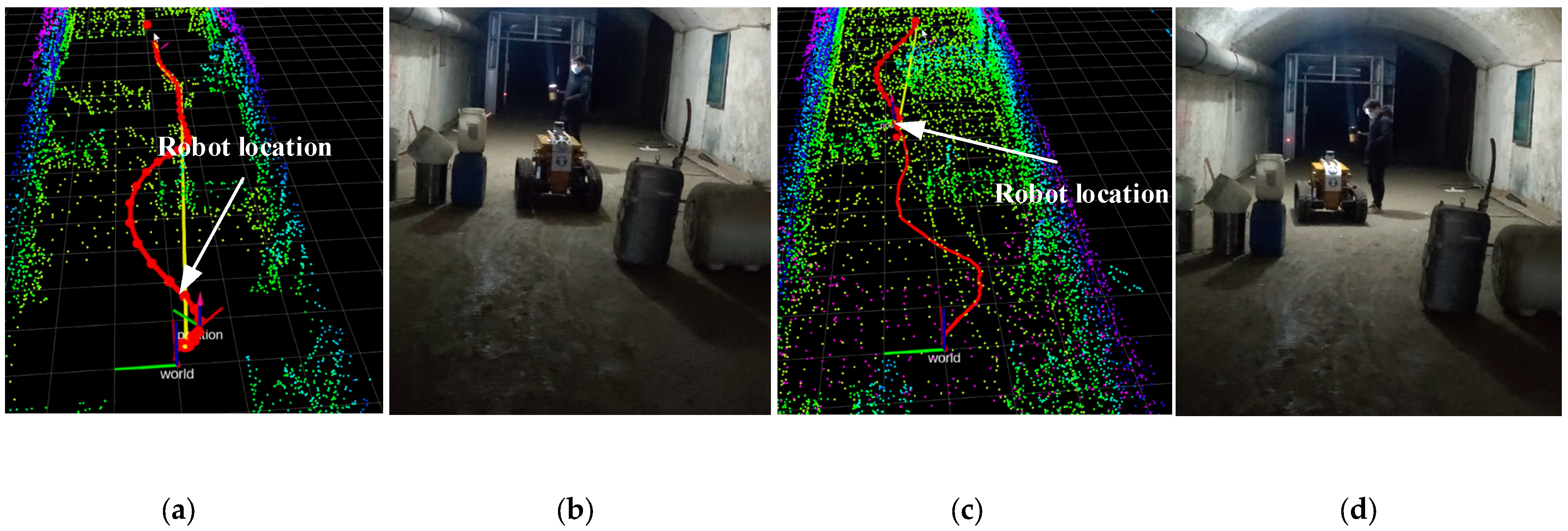
The planning experiments in scenarios combining dynamic and static obstacles are shown in Figure 27. Obstacle 1 is about 3.4 m in front of the robot, and the X-axis and Y-axis distances between obstacle 1 and obstacle 2 are about 1.6 m and 1.1 m. The Y-axis distance between the pedestrian and obstacle 2 is about 2.8 m. The target point is set 14 m in front of the robot for the planning experiment. When the robot is about to cross the blue barrel barrier, the pedestrian walks to the middle of the laneway. At this time, the robot should replan to avoid the pedestrian and reach the end point.
The experimental results of the MINCO trajectory method are shown in Figure 28. Figure 28a shows the better planning results given by the algorithm after being adjusted for the given target point. Figure 28b shows the pedestrian obstacle moving to the middle of the alley. Figure 28c shows the replanning result when a new obstacle is encountered. Figure 28d shows the robot avoiding the pedestrian obstacle.
The experimental results of the Fast-Planner planning algorithm are shown in Figure 29.
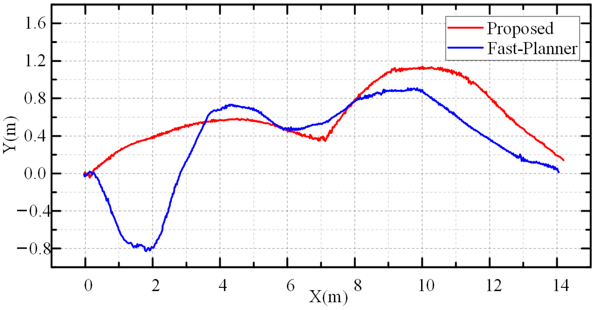
A comparison of the final trajectories of the two algorithms is shown in Figure 30. The MINCO trajectory method performed a total of seven planning passes during the robot movement, with a total planning time of 0.692 s and a robot trajectory length of 14.8 m. The Fast-Planner algorithm performed a total of 438 planning passes throughout the entire process, with a total time of 2.61 s and a robot trajectory length of 15.38 m.
As can be seen from the above data and trajectory comparison, in a complex scenario combining dynamic and static obstacles, the Fast-Planner algorithm will keep planning to find a safe path, so the number of planning times is very large. On the other hand, the MINCO trajectory method can still obtain a smooth trajectory with better performance in many indexes with only seven times of planning.
Combining the multiple experiments above, it can be found that in different scenarios, the planning algorithms based on MINCO trajectories and safe corridors proposed in this paper can complete the planning task within 10 times of planning. And the smoothness of the trajectory, the length of the trajectory, and the planning time are better than the Fast-Planner algorithm.

4.2. Experiments on Trajectory Tracking of CMRRs

The mobile robot platform and test environment used for the test are still the same as those used for the trajectory planning test. A number of scenarios are designed by issuing straight line and sinusoidal curve type trajectories and selecting different terrains and locations in the simulated tunnel to investigate the effect of the MPC tracking algorithm in the real environment. The robot localization information is still given by the LOAM algorithm. The results of PID trajectory tracking were also tested to verify the superiority of the MPC trajectory tracking method proposed in this paper.

4.2.1. Trajectory Tracking Test on a Flat Surface in the Simulated Laneway

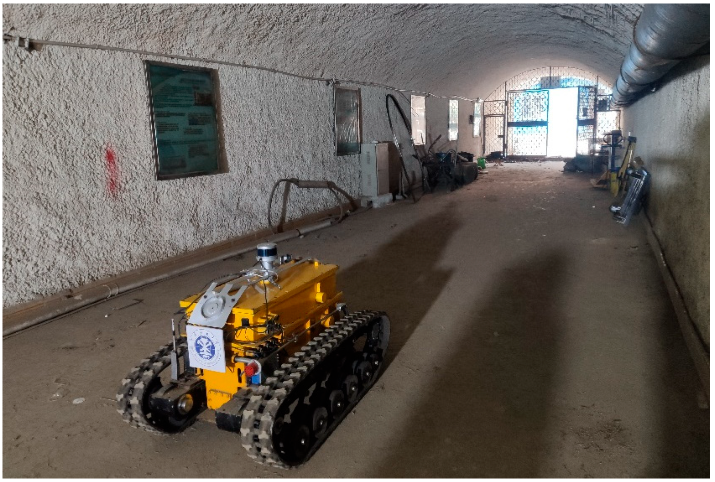
The experiment of a robot tracking linear and sinusoidal curve-type trajectories was first performed sequentially in the flat ground area of the simulated tunnel. The experimental environment is shown in Figure 31.
  • Test 1: Linear trajectory tracking test
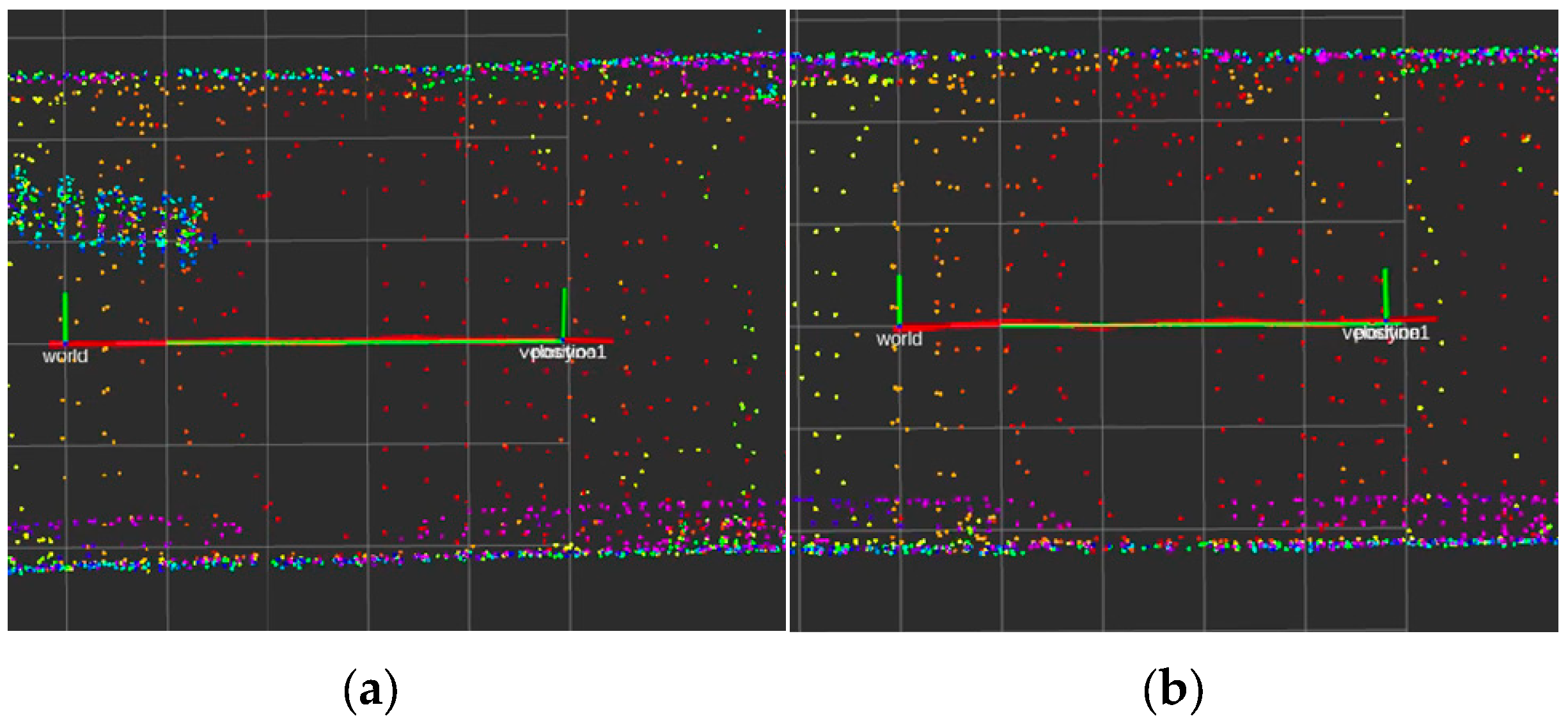
A 4 m long linear trajectory is issued to the direction directly in front of the robot (x-axis). The MPC and PID trajectory tracking algorithms are run separately to compare the tracking effects of the two algorithms. The visualization results of the MPC algorithm and PID algorithm tracking straight line experiments in RVIZ are shown in Figure 32, where the red curve is the actual trajectory of the robot and the green curve is the published desired trajectory.
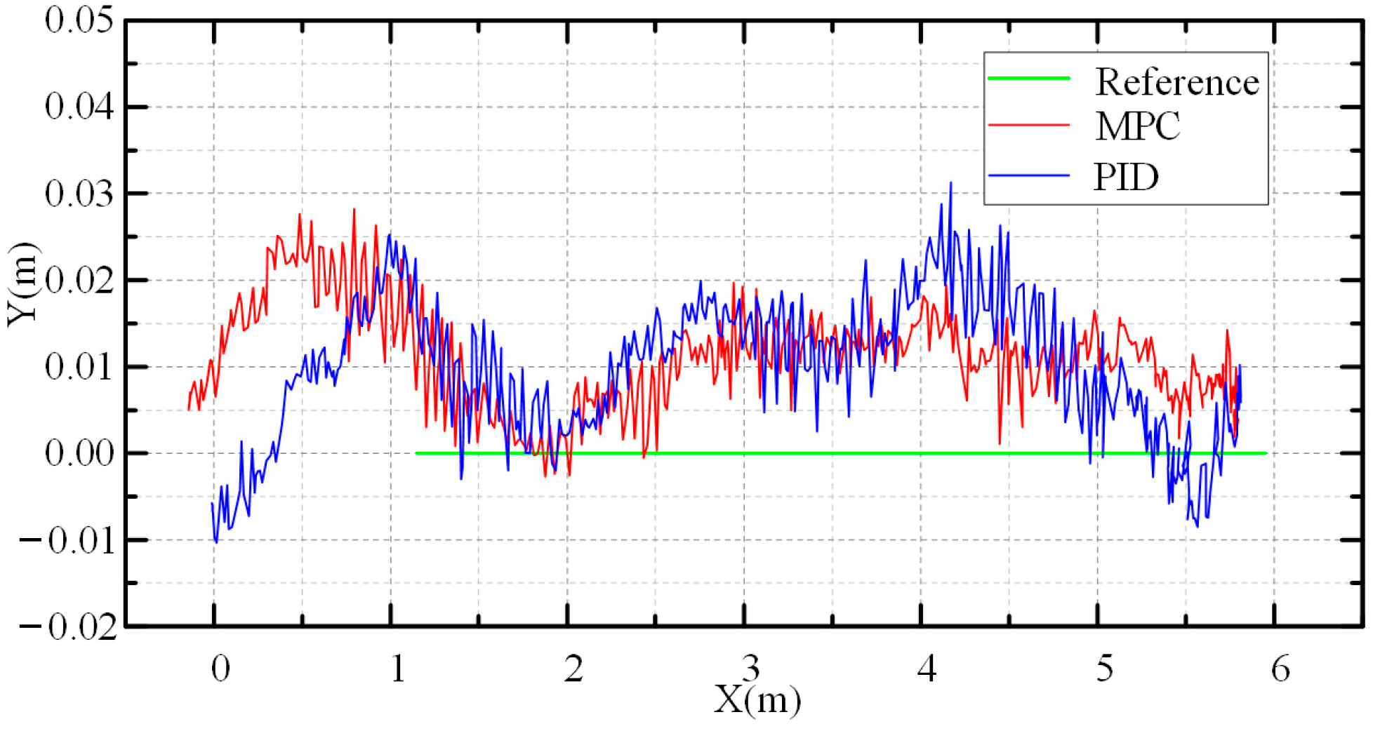
Compare the effect of MPC algorithm and PID algorithm. The motion trajectory comparison graph of the robot moving from the initial point to the target point is shown in Figure 33. The Y-axis error is used as the comparison term. Since the published desired trajectory Y is a constant equal to 0 and X is from 1 m to 5 m, the robot tracking error can be clearly seen. Take the motion trajectory after the robot reaches the desired point, i.e., the trajectory after the X-axis is greater than 1 m for the correlation calculation. The maximum tracking error of the MPC algorithm is 0.041 m, and the standard deviation of the error is 0.008 m. The maximum tracking error of the PID algorithm is 0.041 m, and the standard deviation of the error is 0.01 m.
From the above data and Figure 33, it can be seen that under the tracking control of both algorithms, the robot can track the desired trajectory well. At the same time, the maximum error is only 0.041 m. The difference in standard deviation between the two algorithms is also very small, within 0.002 m.
  • Test 2: Sine curve type trajectory tracking test
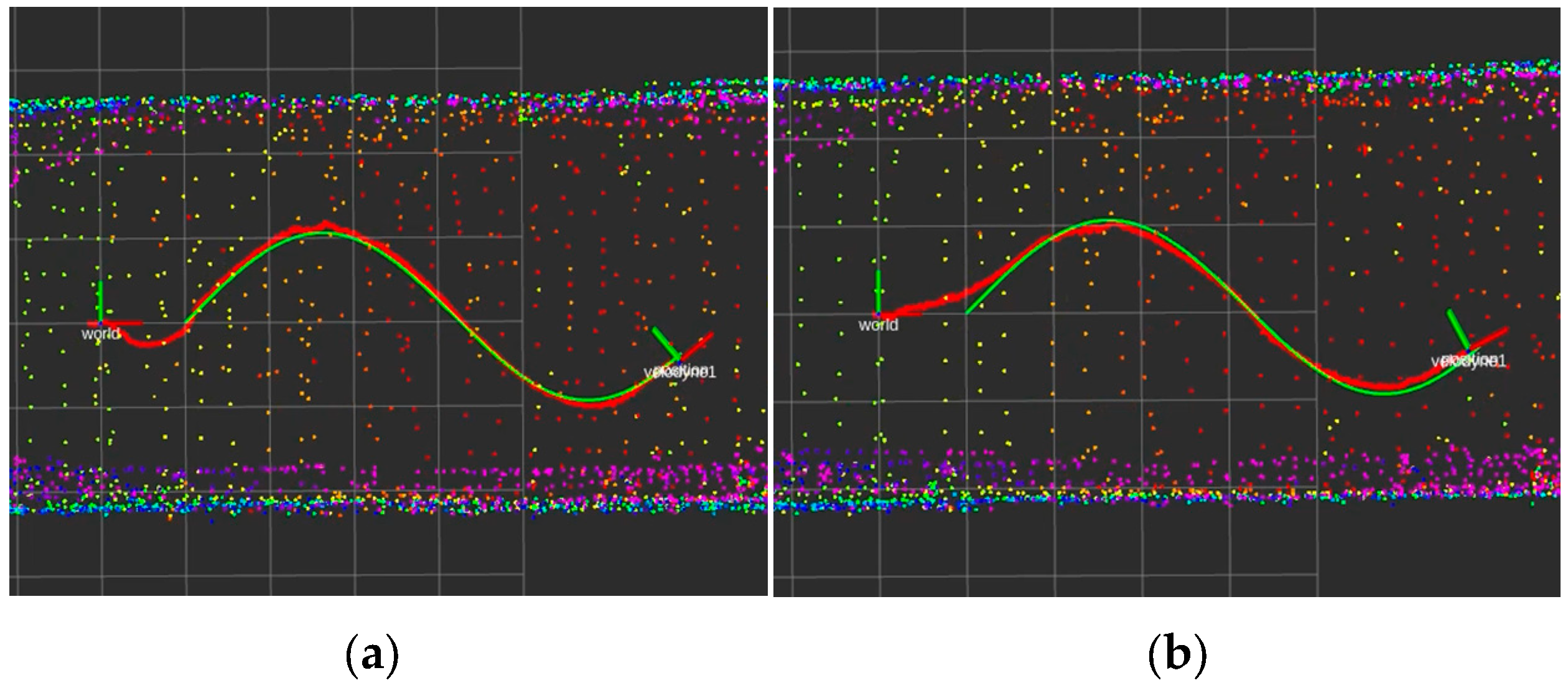
A sinusoidal curve-type trajectory that varies in the positive direction of the X-axis for about one cycle was released 1 m directly in front of the robot. Subsequently, the MPC and PID trajectory tracking algorithms were run separately to compare the trajectory tracking effects of the two algorithms. The result plots in the RVIZ visualization interface when the MPC algorithm and the PID algorithm track the sinusoidal trials are shown in Figure 34, where the red curve is the actual trajectory of the robot and the green curve is the desired trajectory.
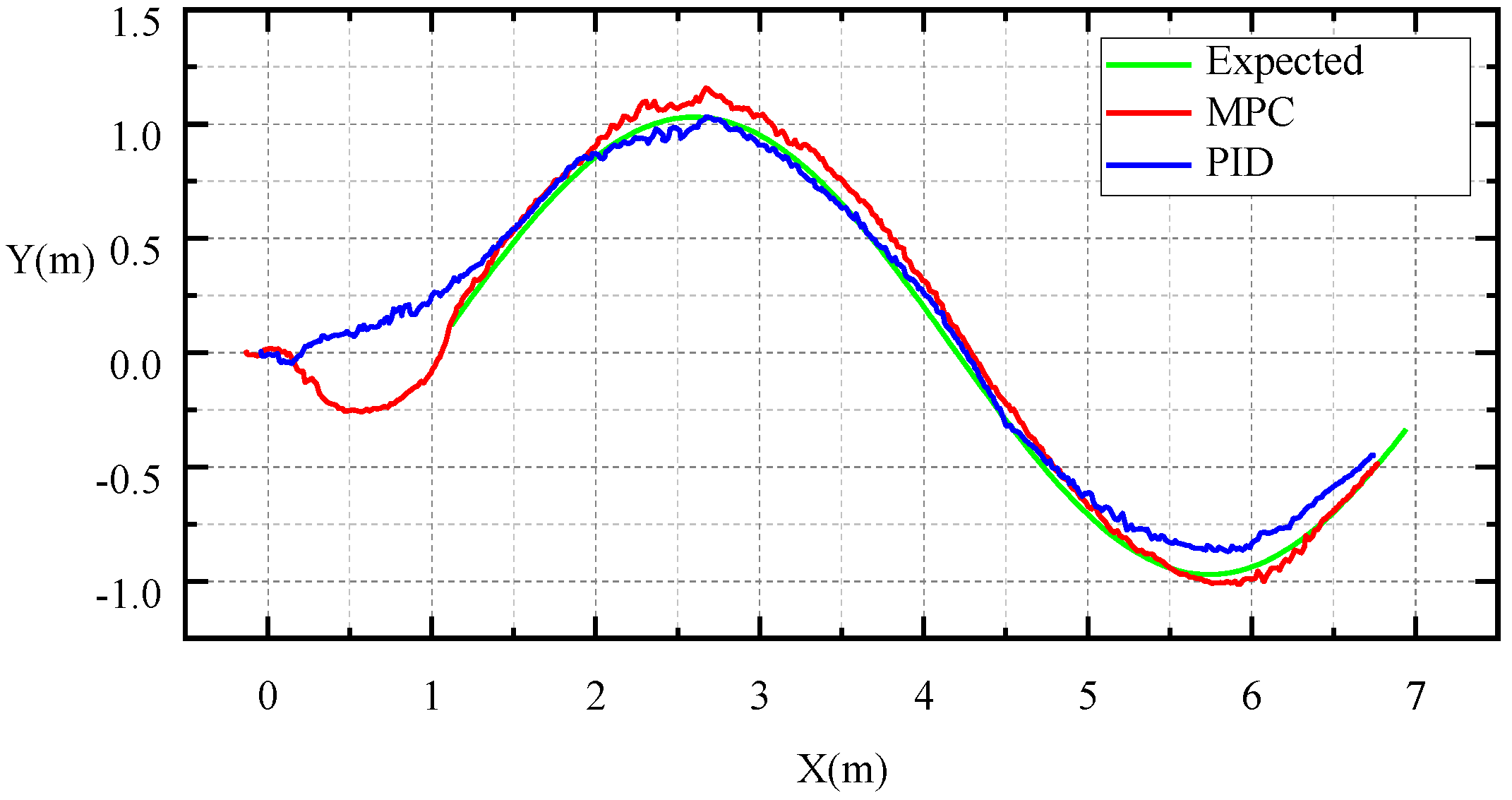
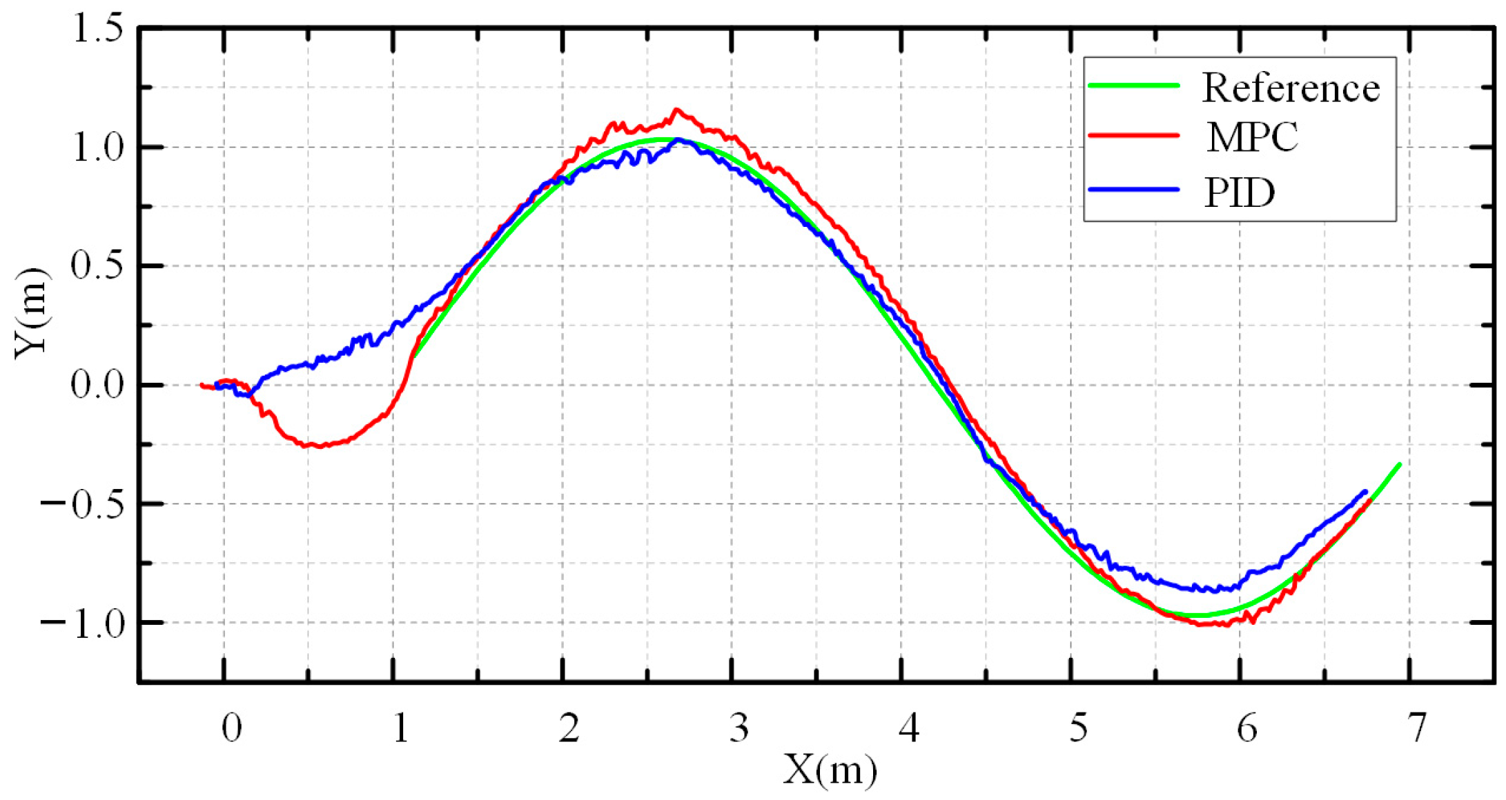
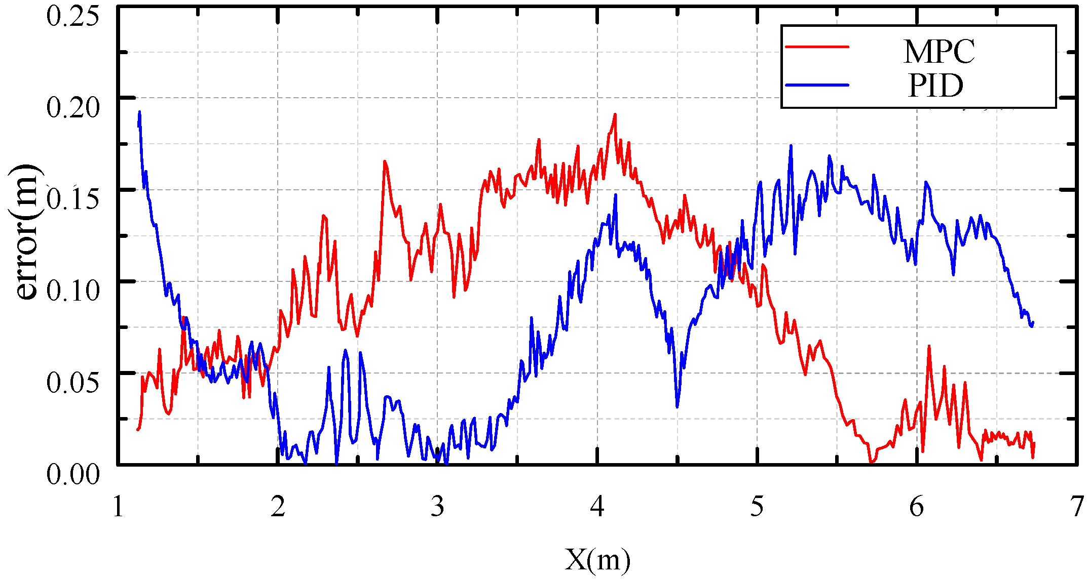
Shown in Figure 35 is the comparison of the motion trajectory of the two algorithms MPC and PID for the robot moving from the initial point to the target point. Figure 36 shows the comparison of the tracking error of the two algorithms. Still, the trajectory after the X-axis is greater than 1 m for the calculation of the relevant indicators, the maximum tracking error of the MPC algorithm is 0.191 m, and the standard deviation of the error is 0.0514 m. The maximum tracking error of the PID algorithm is 0.192 m, and the standard deviation of the error is 0.049 m.
From the above data and Figure 34 and Figure 35, it can be seen that under the tracking control of both algorithms, the robot can track the desired trajectory. And the maximum error is close to 0.2 m, and the difference between the standard deviation of the two algorithms is also very small, within 0.002 m.
The probable reasons for the maximum error approaching 0.2 m are as follows: (1) In the process of tracking the sinusoidal curve-type trajectory, the robot went through several large-scale steerings, which led to a larger cumulative error in the laser odometer, causing the lidar localization algorithm to generate cumulative error, making the tracking error larger. (2) The robot is a tracked differential model, which is prone to side-slip during continuous turns, resulting in larger tracking errors.
Analyze the reasons for the difference in tracking effectiveness between MPC and PID algorithms in tracking sinusoidal curves. PID uses the lateral tracking error as an error feedback term, which is a single-input, single-output controller with the goal of keeping the lateral tracking error as close to zero as possible. On the other hand, MPC predicts the state in the next period of time and solves the most reasonable control quantity at the current moment, so that the robot’s position error when reaching the target position is 0, i.e., the robot’s X- and Y-axis coordinates and the heading angle are as consistent as possible with the desired position of the target point. Therefore, when MPC is tracking the whole sinusoidal curve, it first adjusts the attitude so that the position is basically the same as the given one when it reaches the initial point of the target trajectory. PID, on the other hand, is unable to do so. Anyway, both of the algorithms complete the tracking of the target trajectory.

4.2.2. Trajectory Tracking Test on a Bumpy Road Surface in the Simulated Laneway

The bumpy road surface deep in the simulated laneway is shown in Figure 37. Due to the narrow roadway, the robot can only walk in a straight line and cannot track the sinusoidal curve type trajectory, so only the straight line trajectory tracking test is conducted here.
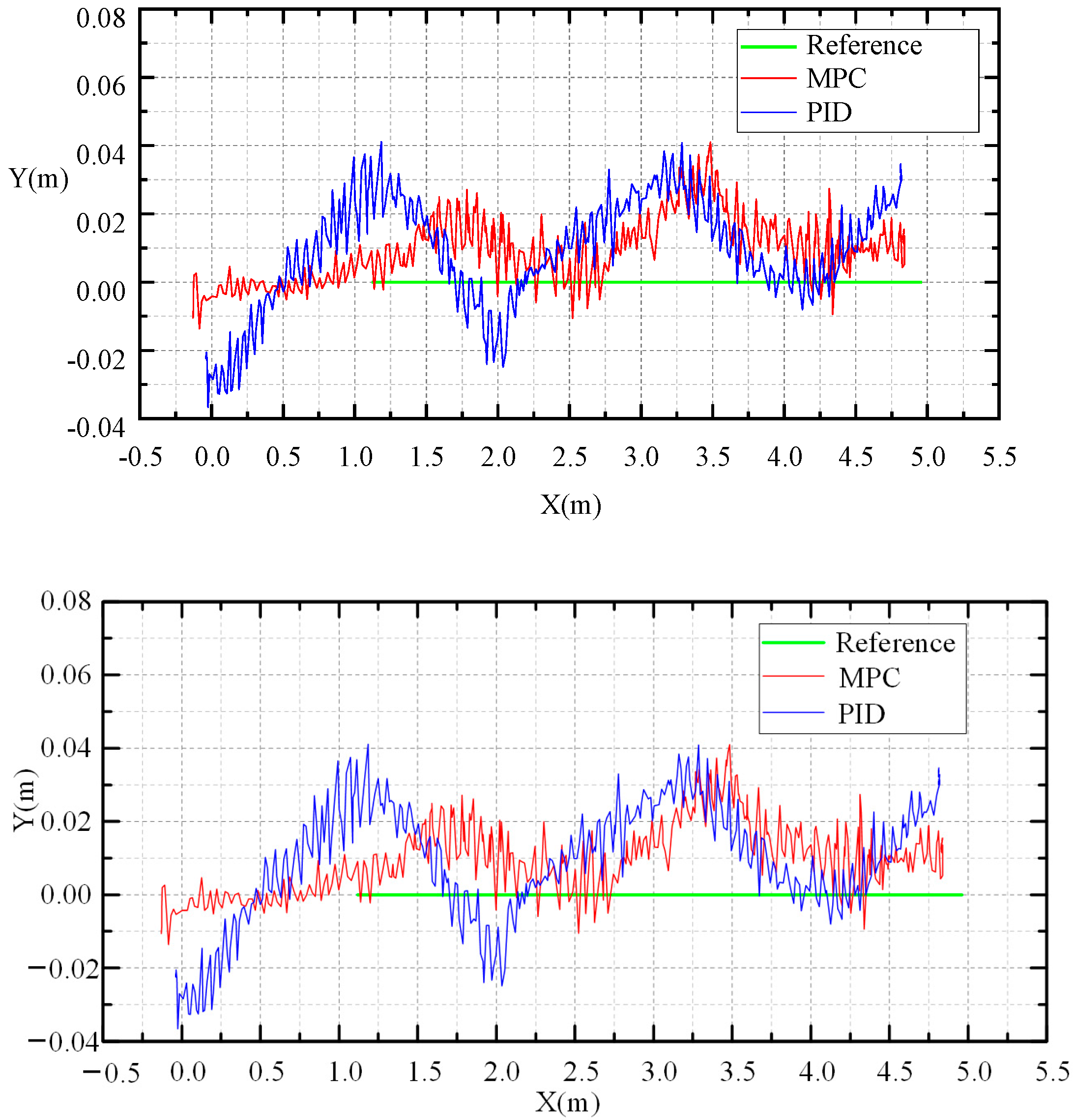
At 1 m directly in front of the robot, a linear trajectory with a length of 5 m is issued in the positive direction towards the X-axis. The MPC and PID trajectory tracking algorithms are run separately to compare the tracking effect of the two algorithms. The RVIZ visualization results of the MPC algorithm and the PID algorithm for tracking a straight-line trial in this scenario are shown in Figure 38.
Shown in Figure 39 is a comparison of the motion trajectories of the robot executing the two algorithms MPC and PID from the initial point to the target point in this scenario. The maximum tracking error of the MPC algorithm is 0.028 m, and the standard deviation of the error is 0.0045 m. The maximum tracking error of the PID algorithm is 0.031 m, and the standard deviation of the error is 0.0065 m.
From the above data and Figure 39, it can be seen that under the tracking control of the two algorithms, the robot is able to track the desired trajectory well, with the maximum error being around 0.03 m. The difference in the standard deviation of the two algorithms is also very small, still within 0.002 m. The standard deviation of the two algorithms is also very small.
In summary, both the MPC trajectory tracking algorithm and the PID algorithm in this paper are capable of tracking a given trajectory. However, when tracking sinusoidal continuous curves, the tracking results of the MPC algorithm are more in line with the position of the desired trajectory, responding to the heading angle of the target trajectory from the first point of the target trajectory, and the turning scenarios in the tunnel are safer, with better overall results. After the many tests shown above, the MPC in this paper is successfully applied to tracked CMRR, which has a certain practical application value.

5. Conclusions

This paper researches the trajectory planning and tracking technology of CMRR and puts forward the planning algorithm based on MINCO trajectory in a safety corridor with a tracking algorithm based on MPC. A large number of field experiments were carried out in the simulated laneway based on a crawler-type CMRR platform, which verifies that the methods of this paper are also applicable to the field environment, and it has a certain value of practical application. The main research work and results of this paper are as follows:
(1) The MINCO trajectory class and its spatio-temporal deformation are derived in detail, and the MINCO trajectory is used to generate the optimal control trajectory under the constraints of a downhole environment. The planning effects of the MINCO trajectory method and the Fast-Planner algorithm are compared through several field experiments. The results show that the trajectories of the MINCO trajectory method are smoother and shorter, accomplishing the same planning task at a smaller cost; planning tasks were completed in fewer than 10 planning sessions for each scenario, which proves that the proposed algorithm is better adapted to the complex environment of underground coal mines.
(2) The kinematic model of the experimental platform of a tracked coal mine robot is established. The MPC trajectory tracking method is further designed. The field tests prove that the tracking error is always less than 0.05 m, which is more adaptable to the tracking of different paths compared with the PID algorithm.
(3) A highly reliable trajectory planning and tracking system that meets the performance requirements is provided for CMRRs, which can be used for autonomous navigation and remote control assisted driving. The effectiveness of the planning and tracking system is verified through a large number of field tests, which provide key technical support for the application of CMRRs.

Author Contributions

Conceptualization, M.L. and G.Z.; methodology, M.L. and W.H.; software, K.H.; validation, K.H., E.H. and C.T.; formal analysis, M.L.; investigation, M.L. and G.Z.; resources, G.Z. and E.H.; data curation, W.H.; writing—original draft preparation, K.H. and W.H.; writing—review and editing, M.L.; visualization, W.H.; supervision, M.L. and G.Z.; project administration, G.Z., funding acquisition, M.L. All authors have read and agreed to the published version of the manuscript.

Funding

This research was funded by the National Natural Science Foundation of China (grant number: 52304183, 52274159), the Joint Open Fund of State Key Laboratory of Robotics (grant number: 2022-KF-22-05), and the Natural Science Foundation of Jiangsu Province for Youths (grant number: BK20210497).

Institutional Review Board Statement

Not applicable.

Informed Consent Statement

Not applicable.

Data Availability Statement

The data are unavailable.

Conflicts of Interest

The authors declare no conflict of interest.

References

  1. Ge, S.R. Present situation and development direction of coal mine robots. China Coal 2019, 45, 18–27. [Google Scholar]
  2. Cai, G.S.; Liu, H.J.; Feng, J.W.; Xu, L.W.; Yin, G.D. Review on the research of motion planning and control for intelligent vehicles. J. Automot. Saf. Energy 2021, 12, 279–297. [Google Scholar]
  3. Liu, J.Y. Research on Smooth Path Planning and Trajectory Tracking of Mobile Robot. Master’s Thesis, Beijing Jiaotong University, Beijing, China, 2022. [Google Scholar]
  4. Bao, J.S.; Zhang, M.Y.; Ge, S.R.; Liu, Q.; Yuan, X.M.; Wang, M.S.; Yin, Y.; Zhao, L. Underground driveless path planning of trackless rubber tyred vehicle based on improved A* and artificial potential field algorithm. J. China Coal Soc. 2022, 47, 1347–1360. [Google Scholar]
  5. Kavraki, L.E.; Svestka, P.; Latombe, J.C.; Overmars, M.H. Probabilistic roadmaps for path planning in high-dimensional con-figuration spaces. IEEE Trans. Robot. Autom. 1996, 12, 566–580. [Google Scholar] [CrossRef]
  6. Peng, C.; Lavalle, S.M. Resolution complete rapidly-exploring random trees. In Proceedings of the 2002 IEEE Inter-National Conference on Robotics and Automation, Washington, DC, USA, 11–15 May 2002; IEEE: Piscataway, NJ, USA, 2002; pp. 267–272. [Google Scholar]
  7. Karman, S.; Frazzoli, E. Sampling-based algorithms for optimal motion planning. Int. J. Robot. Res. 2011, 30, 846–894. [Google Scholar] [CrossRef]
  8. Yan, Y.; Li, C.S.; Tang, F.M. Lane-changing trajectory planning of the autonomous vehicle based on the quintic polynomial model. J. Mach. Des. 2019, 36, 42–47. [Google Scholar]
  9. Chen, J.J.; Zhao, P.; Mei, T.; Liang, H. Lane Change Path Planning Based on Piecewise Bezier Curve for Autonomous Vehicle. In Proceedings of the IEEE International Conference on Vehicular Electronics and Safety, ICVES 2013, Dongguan, China, 28–30 July 2013; IEEE: Piscataway, NJ, USA, 2013; pp. 17–22. [Google Scholar]
  10. Ji, W.C.; Curry, R.E.; Elkaim, G.H. Continuous Curvature Path Generation Based on Bézier Curves for Autonomous Vehicles. IAENG Int. J. Appl. Math. 2010, 40, 91–101. [Google Scholar]
  11. Choi, J.W.; Curry, R.; Elkaim, G. Path Planning Based on Bezier Curve for Autonomous Ground Vehicles. In Proceedings of the World Congress on Engineering and Computer Science 2008, WCECS, San Francisco, CA, USA, 22–24 October 2008; IEEE: Piscataway, NJ, USA, 2009; pp. 158–166. [Google Scholar]
  12. Bae, I.; Moon, J.; Park, H.; Kim, J.H.; Kim, S. Path Generation and Tracking Based on a Bezier Curve for a Steering Rate Controller of Autonomous Vehicles. In Proceedings of the 16th International IEEE Conference on Intelligent Transportation Systems (ITSC 2013), The Hague, The Netherlands, 6–9 October 2013; IEEE: Piscataway, NJ, USA, 2013; pp. 436–441. [Google Scholar]
  13. Qu, P.R.; Li, L.; Ren, X.K.; Jin, L. B-spline Curve based Trajectory Planning for Autonomous Vehicles. Comput. Knowl. Technol. 2016, 12, 235–237. [Google Scholar]
  14. Maekawa, T.; Noda, T.; Tamura, S.; Ozaki, T.; Machida, K.-I. Curvature continuous path generation for autonomous vehicle using B-spline curves. Comput. Aided Des. 2010, 42, 350–359. [Google Scholar] [CrossRef]
  15. Boryga, M.; Kołodziej, P.; Gołacki, K. Application of Polynomial Transition Curves for Trajectory Planning on the Headlands. Agriculture 2020, 10, 144. [Google Scholar] [CrossRef]
  16. Liu, X.; Chen, C.Z.; Wang, R.; Tang, R.J. Trajectory tracking control of mobile robot based on HJI. J. Sichuan Univ. Sci. Eng. 2022, 35, 66–73. [Google Scholar]
  17. Zhu, W.L.; Huang, J.J.; Zhou, Y.P. Research on self-guided AGV motion control based on fuzzy adaptive PID. Sci. Technol. Innov. 2023, 220–223. [Google Scholar]
  18. Li, W.W.; Yuan, S.; Zhou, X.R. AGV trajectory tracking controller based on visual neuron PID. Modul. Mach. Tool Autom. Manuf. Tech. 2022, 56–61. [Google Scholar]
  19. Ha, T.K.D.; Nguyen, M.C.; Vo, H.T.; Tran, V.M.; Bui, A.D. Trajectory tracking control for four-wheeled omnidirectional mobile robot using Backstepping technique aggregated with sliding mode control. In Proceedings of the 2019 First International Symposium on Instrumentation, Control, Artificial Intelligence, and Robotics (ICA-SYMP), Bangkok, Thailand, 16–18 January 2019; IEEE: Piscataway, NJ, USA, 2019; pp. 131–134. [Google Scholar]
  20. Wang, J.; Cheng, H.; Jiang, R.J.; Cai, Y. Adaptive trajectory tracking of tracked robot based on sliding mode feedback. Modular Mach. Tool Autom. Manuf. Tech. 2023, 33, 25–28. [Google Scholar]
  21. Minh, T.V. Nonlinear Model Predictive Controller and Feasible Path Planning for Autonomous Robots. Open Comput. Sci. 2016, 6, 178–186. [Google Scholar] [CrossRef]
  22. Li, Y.Z.; Li, G.; Zhang, Z.H. Lateral tracking control of a driverless four-wheel steering vehicle under extreme conditions. J. Chongqing Univ. Technol. 2023, 37, 66–74. [Google Scholar]
  23. Shi, Z.X.; Feng, J.B.; Wang, H.X. Research on intelligent vehicle path tracking based on MPC and Fuzzy Control. Veh. Power Technol. 2022, 2184, 7–11. [Google Scholar]
  24. Yin, C.; Wang, S.; Gao, J.; Li, X. Trajectory tracking for agricultural tractor based on improved fuzzy sliding mode control. PLoS ONE 2023, 18, e0283961. [Google Scholar] [CrossRef]
  25. Fliess, M.; Lévine, J.; Martin, P.; Rouchon, P. Flatness and defect of non-linear systems: Introductory theory and examples. Int. J. Control 1995, 61, 1327–1361. [Google Scholar] [CrossRef]
  26. Van, N.M.J.; Murray, R.M. Real-time trajec-tory generation for differentially flat systems. Int. J. Robust Nonlinear Control 1998, 8, 995–1020. [Google Scholar]
  27. Martin, P.; Murray, R.M.; Rouchon, P. Flat systems, equivalence and trajectory generation. Model. Identif. Control Robot. 2009, 92, 313–345. [Google Scholar]
  28. Ryu, J.C.; Agrwal, S.K. Differential flatness-based robust control of mobile robots in the presence of slip. Int. J. Robot. Res. 2011, 30, 463–475. [Google Scholar] [CrossRef]
  29. Wang, Z.; Zhou, X.; Xu, C.; Gao, F. Geometrically Constrained Trajectory Optimization for Multicopters. IEEE Trans. Robot. 2022, 38, 3259–3278. [Google Scholar] [CrossRef]
  30. Wang, Z.P. A Geometrical Approach to Multicopter Motion Planning. Master’s Thesis, Zhejiang University, Zhejiang, China, 2022. [Google Scholar]
  31. Zhang, J.; Singh, S. LOAM: Lidar odometry and mapping in real-time. In Proceedings of the Robotics: Science and Systems; The MIT Press: Rome, Italy, 2014; Volume 2, pp. 1–9. [Google Scholar]
  32. Zhou, B.; Gao, F.; Wang, L.; Liu, C.; Shen, S. Robust and Efficient Quadrotor Trajectory Generation for Fast Autonomous Flight. IEEE Robot. Autom. Lett. 2019, 4, 3529–3536. [Google Scholar] [CrossRef]
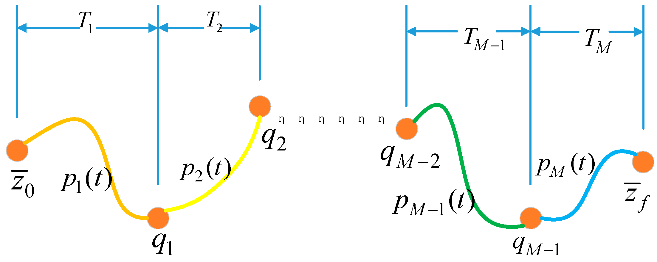
Figure 1. The optimal trajectory diagram of path point and time vector parameterization.
Applsci 13 09789 g001
Figure 2. Schematic diagram of voxel map.
Applsci 13 09789 g002
Figure 3. Ellipsoid shrinkage process.
Applsci 13 09789 g003
Figure 4. Process of finding polyhedron.
Applsci 13 09789 g004
Figure 5. Polyhedron set.
Applsci 13 09789 g005
Figure 6. Setting the boundary box.
Applsci 13 09789 g006
Figure 7. Polyhedron collection after setting the bounding box.
Applsci 13 09789 g007
Figure 8. Safe corridor.
Applsci 13 09789 g008
Figure 9. Trajectory processing outside the safe area.
Applsci 13 09789 g009
Figure 10. Spherical constraint variable mapping.
Applsci 13 09789 g010
Figure 11. Convex polyhedron constraint variable mapping.
Applsci 13 09789 g011
Figure 12. Flow chart of planning method based on MINCO trajectory.
Applsci 13 09789 g012
Figure 13. Robot kinematics model.
Applsci 13 09789 g013
Figure 14. Test robot platform and test environment.
Applsci 13 09789 g014
Figure 15. Single obstacle scenario: (a) site environment map; (b) RVIZ 3D point cloud map. “world” represents the world coordinate, the red axis is the X-axis, the green axis is the Y-axis, the blue axis is the Z-axis, and the coordinate “position” indicates the robot position.
Applsci 13 09789 g015
Figure 16. Experimental process of MINCO trajectory algorithm in single obstacle scenarios: (a) planning result; The blue curve is the target trajectory planned by the algorithm, and the light-blue polyhedron is the safety corridor. (b) actual pose.
Applsci 13 09789 g016
Figure 17. Test process of Fast-Planner algorithm in single obstacle scenario: (a) start planning; (b) replanning; (c) trajectory execution; (d) actual pose relationship. The red curve is the target trajectory planned by the algorithm.
Applsci 13 09789 g017
Figure 18. Comparison between MINCO trajectory algorithm and Fast-Planner algorithm for single obstacle trajectory.
Applsci 13 09789 g018
Figure 19. Multiple obstacle scenarios: (a) site environment. (b) Rviz 3D point cloud map.
Applsci 13 09789 g019
Figure 20. Experimental results of MINCO trajectory method in multiobstacle scenarios: (a) start planning; (b) trajectory execution; (c) entering the obstacle zone; (d) leaving the obstacle zone.
Applsci 13 09789 g020
Figure 21. Experimental process of Fast-Planner algorithm in multiobstacle scenarios: (a) start planning; (b) trajectory execution; (c) entering the obstacle zone; (d) leaving the obstacle zone.
Applsci 13 09789 g021
Figure 22. Comparison of multiple obstacle trajectories between MINCO trajectory method and Fast-Planner algorithm.
Applsci 13 09789 g022
Figure 23. Right-angle turn scenario test.
Applsci 13 09789 g023
Figure 24. Experimental process of MINCO trajectory method in right-angle bend scenes (a) start planning; (b) replan; (c) entering the bend; (d) leaving the bend.
Applsci 13 09789 g024
Figure 25. Fast-Planner algorithm test process in right-angle bend scenarios.
Applsci 13 09789 g025
Figure 26. Trajectory of the proposed algorithm in right-angle bend scenario.
Applsci 13 09789 g026
Figure 27. Dynamic and static obstacle combination scenario.
Applsci 13 09789 g027
Figure 28. Experimental results of dynamic scene by MINCO trajectory method: (a) start planning; (b) pedestrian presence; (c) replan; (d) avoiding pedestrians.
Applsci 13 09789 g028
Figure 29. Experimental results of dynamic scene by Fast-Planner trajectory method: (a) start planning; (b) pedestrian presence; (c) replan; (d) avoiding pedestrians.
Applsci 13 09789 g029
Figure 30. Comparison of dynamic obstacle trajectories between MINCO trajectory method and Fast-Planner algorithm.
Applsci 13 09789 g030
Figure 31. Flat ground test in simulated laneway.
Applsci 13 09789 g031
Figure 32. Linear tracking test results: (a) MPC algorithm tracking results, (b) PID algorithm tracking results. The red curve is the actual trajectory of the robot and the green curve is the published desired trajectory.
Applsci 13 09789 g032
Figure 33. Comparison of MPC and PID in linear motion trajectories.
Applsci 13 09789 g033
Figure 34. Sine curve tracking test results: (a) MPC algorithm tracking results (b) PID algorithm tracking results. The red curve is the actual trajectory of the robot and the green curve is the desired trajectory.
Applsci 13 09789 g034
Figure 35. Comparison diagram of MPC and PID sinusoidal curve motion trajectories.
Applsci 13 09789 g035aApplsci 13 09789 g035b
Figure 36. Comparison diagram of MPC and PID tracking errors.
Applsci 13 09789 g036
Figure 37. Simulated roadway bumpy road test environment.
Applsci 13 09789 g037
Figure 38. Linear tracking test results on bumpy road: (a) MPC algorithm tracking results, (b) PID algorithm tracking results. The red curve is the actual trajectory of the robot and the green curve is the desired trajectory.
Applsci 13 09789 g038
Figure 39. Comparison of MPC and PID motion trajectories on bumpy roads.
Applsci 13 09789 g039
Disclaimer/Publisher’s Note: The statements, opinions and data contained in all publications are solely those of the individual author(s) and contributor(s) and not of MDPI and/or the editor(s). MDPI and/or the editor(s) disclaim responsibility for any injury to people or property resulting from any ideas, methods, instructions or products referred to in the content.