Abstract
A good understanding of historical change rates is a key requirement for effective coastal zone management and reliable predictions of shoreline evolution. Historical shoreline erosion for the coast of Guardamar del Segura (Alicante, Spain) is analyzed based on aerial photographs dating from 1930 to 2022 using the Digital Shoreline Analysis System (DSAS). This area is of special interest because the construction of a breakwater in the 1990s, which channels the mouth of the Segura River, has caused a change in coastal behavior. The prediction of future shorelines is conducted up to the year 2040 using two models based on data analysis techniques: the extrapolation of historical data (including the uncertainty of the historical measurements) and the Bruun-type model (considering the effect of sea level rises). The extrapolation of the natural erosion of the area up to 1989 is also compared with the reality, already affected by anthropic actions, in the years 2005 and 2022. The construction of the breakwater has accelerated the erosion along the coast downstream of this infrastructure by about 260%, endangering several houses that are located on the beach itself. The estimation models predict transects with erosions ranging from centimeters (±70 cm) to tens of meters (±30 m). However, both models are often overlapping, which gives a band where the shoreline may be thought to be in the future. The extrapolation of erosion up to 1989, and its subsequent comparison, shows that in most of the study areas, anthropic actions have increased erosion, reaching values of more than 35 m of shoreline loss. The effect of anthropic actions on the coast is also analyzed on the housing on the beach of Babilonia, which has lost around 17% of its built-up area in 40 years. This work demonstrates the importance of historical analysis and predictions before making any significant changes in coastal areas to develop sustainable plans for coastal area management.
1. Introduction
Coasts are valuable and vulnerable environments that provide numerous ecosystem services and support human populations in different ways [1]. It is estimated that sandy beaches make up approximately one-half of the world’s ice-free coastline [2]. According to the United Nations, approximately 10% of the world’s population currently lives in coastal areas that are less than 10 m above sea level, and about 40% lives within 100 km of the coast [3]. These areas are residentially, touristically and economically attractive; thus, they are becoming densely populated, but the concentration of infrastructures due to intense anthropic activity (i.e., ports, cities and resorts) puts additional stress on the coastal environment, sometimes pressing it to its limits [4].
Coastal zones are particularly vulnerable to natural erosive processes due to factors like wave action or storm events [5]. These processes can lead to the loss of land, degradation of coastal ecosystems, and increased risks for human settlements and infrastructure. The problem is emphasized when anthropic constructions modify coastal dynamics in some way, even though their primary objective is to protect the coast from erosion due to natural phenomena [6,7,8]. While these structures (i.e., harbors, channels or breakwaters) may provide immediate protection against erosion, they can disrupt the natural movement of sediment along the coastline, leading to unintended consequences [9,10]. Many of these hard structures were built from the 1950s to the 2000s, without accurate studies of the effects on coastal sediment dynamics and flora and fauna [1]. In contrast, in the last two or three decades, management strategies have focused on soft methods such as artificial beach nourishment, revegetation of dunes or bioengineering [11,12]. For example, some researchers have found a relationship between increased shoreline erosion in areas around the mouths of dammed rivers and in areas with high population densities in the Gulf of California [13]. Research conducted on the East Coast of South Korea found that the artificial structures constructed along the coast have not completely solved or stopped erosion but shifted it from one location to another [14]. On the contrary, work by Skilodimou et al. [15] shows how coastlines have been enhanced by 40% over the last 76 years due to human interventions, in this case, earth filling.
The effects of climate change on coastal regions are critical due to their exposure to rising sea levels, increased storm intensity and changes in oceanic and atmospheric conditions [16]. In general, rising sea levels can be a significant factor in shoreline changes [17]. Higher water levels mean that waves and storm surges can reach farther inland, eroding coastlines and flooding low-lying areas. This can result in the loss of beaches, dunes and other coastal landforms, which can lead to feedback loops, e.g., as coastal areas erode, sediment may be lost, reducing natural coastal barriers and exacerbating erosion. This, in turn, can increase vulnerability to coastal hazards. Changes in ocean wave characteristics, including alterations in wave height, period and direction, can further impact coastal erosion, sediment transport and stability. In addition to this, storms, including hurricanes and tropical cyclones, can cause significant changes due to intense erosion and the transportation of large amounts of sediment along the coastline [18]. An example is the work of Simeone et al. [19], who demonstrate that the beaches studied in Western Sardinia (Italy) show greater changes when faced with consecutive storms and not with an isolated one. These climate change impacts can lead to the loss of coastal land, damage to infrastructure and the displacement of communities. For these reasons, the analysis of the long-term effects of anthropic actions in past cases, in combination with information on the adverse effects of climate change (both at the global and regional levels), is fundamental to ensure the long-term sustainability and resilience of the new actions to be taken.
The aims of this work carried out in Guardamar del Segura, Alicante (Spain) are as follows: (1) analyze the historical evolution of the shoreline from 1930 to 2022, taking into account different anthropic constructions; (2) study the effects of these constructions on the erosion rates of the shoreline and a cliff dune; (3) evaluate the loss of built surface (houses) due to changes in coastal dynamics; (4) estimate the shoreline situation for the year 2040 with the information from available data and the use of two prediction models based on historical recession rates and changes in sea level; and (5) compare, with the use of these computational models, the positions that the coastline would have had in the years 2005 and 2022 without the constructions carried out in the area. The results and methodology provided by this work can be used as the basis for coastal planning and management, especially in areas with key infrastructures.
2. Study Area
This work focuses on the coastline of Guardamar del Segura located in the southeast of Alicante, Spain, on the Mediterranean coast (see Figure 1). The area has a population of more than 16,000 inhabitants, and the main economic activity in the region is summer tourism. The studied coast includes the beaches of Los Viveros (corresponding to zone B in Figure 1c) and Babilonia (zone C in Figure 1c). These two beaches have an actual length of 2.7 km and an average width of 12 m, reaching a maximum of 35 m. They are open beaches of golden sand with a grain size of around 0.27 mm [20], which is between fine and coarse sand.
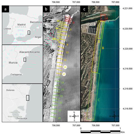
Figure 1.
(a) Location of the study area. (b) Orthomosaic of the coast in 1930 and details of the transects used in the study. (c) Orthophoto of the coast in 2022. Note that the coordinates used are UTM ETRS89 H30N.
Guardamar del Segura coast is a fetch-limited environment with a predominance of sea waves. This coast is an environment with small astronomical tides (as is common in the Mediterranean) that oscillate about 0.3 m (SIMAR data from Puertos del Estado [21]). However, the so-called meteorological tides can reach up to 0.45 m. The dominant wave direction is northeast, creating a net N-S-oriented coastal current. Significant wave heights in this area, from 1958 to 2023, are 50.80% of the time between 0 and 0.5 m, 37.52% between 0.5 and 1 m, 8.7% between 1.0 and 1.5 m, 2.06% between 1.5 and 2.0 m and the remaining 0.92% between 2.0 and 3.5 m [21]. It should be noted that according to the available data [21], the maximum monthly values up to 1970 did not exceed 3 m of significant height. In the 1980s, there were already some peaks that exceeded 4 m, a trend that remained constant with peaks between 2.5 m and 4 m until 2010, but with an average value of around 2 m. However, in the last 13 years, the average has risen around 3 m with some peaks in 2019 of almost 7 m. The latter peak is due to the large Isolated Depression at High Levels (DANA in Spanish) that occurred in the area in 2019 [22]. As for the peak period, the histogram is centered on the 5–6 s interval (23.94% of the time), distributed on the 2–4 s interval (29.12%) and then on the 4–5 s interval (19.59%), 6–7 s interval (17.89%) and 7–10 s interval (17.43%).
According to the latest data published by the Intergovernmental Panel on Climate Change (IPCC), the trend of accelerating sea level rise in the Mediterranean is consistent [23]. However, there are important differences depending on the methods and time horizons used in the analyses. In general, the accepted sea level rise referred to in the 20th century was 1.4 ± 0.2 mm yr−1 [24]. However, by 2050, it is estimated that the sea level may rise between 0.52 and 1.22 m above the mean relative sea level between 1996 and 2014. The relative sea level rise from 1927 to 2012 in Alicante was 1.28 ± 0.5 mm yr−1 [25].
This coastline has a long history of anthropogenic actions since the 18th century. The dune system in this area was left unfixed due to the massive felling of trees for the fishing industry during the 18th century. This meant that for a long time, the town of Guardamar was “threatened” by the movements of the dunes. From 1900 to 1930, the engineer Mira y Botella directed the reforestation of the area, which reduced the mobility of the dunes and, therefore, prevented the burial of the town. The houses of Babilonia (zone C in Figure 1) did not respond to the predatory model of the urbanism of the second half of the last century around the Spanish Levante. On the contrary, they had an environmental function and fit perfectly with the coastal physiognomy of the municipality in the 1930s. The number of houses increased until the end of the 1970s and remained constant until the 2000s, but since then, houses started to naturally and progressively collapse due to marine action. See Figure 2 for some photographs of the area since 2010.
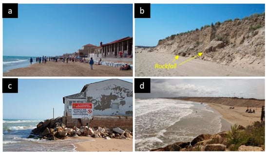
Figure 2.
(a) View from north of Babilonia Beach on 2 April 2010. (b) View of Los Viveros artificial dune on 2 April 2010. (c) View from north of Babilonia Beach on 5 May 2021. (d) View from north of Los Viveros Beach and artificial dune on 13 August 2021.
The main period of anthropic actions began in the mid-1970s and lasted about 20/25 years. In the 1970s, a small groin was built in the southern part of the mouth of the Segura River, which was completed in the mid-1980s with the construction of a larger groin in the northern part. In the period between 1987 and 1988, a large dredging of the mouth of the Segura River was carried out. Between 1990 and 1994, to reduce the risk of flooding, its mouth was channeled by means of a 525 m breakwater with an east and northeast orientation (zone A in Figure 1c), the opposite of all those built in the Spanish Levante [26]. This orientation stops the longitudinal transport of sediments from the north and blocks the outflow of sediments transported by the Segura River [7]. This forces the “Confederación Hidrográfica del Segura (CHS)” to schedule periodic dredging due to sediment accumulation that, if not executed, could cause breakage of the breakwater [27]. A volume of 14,000 m3 of material extracted in the works of the early 1990s was used to raise Viveros beach (zone B in Figure 1c), and the rest of the material was used to raise other beaches to the south of the area of this study. Between 1996 and 1999, the Guardamar marina was built. In this project, a volume of sludge of approximately 200,000 m3 was obtained, basically sand, with a low proportion of fines, very similar to that which makes up the current dune system. This sediment was dumped on a foredune originating an artificial dune (with the appearance of a small cliff) about 500 m long and of variable height (zone D in Figure 1) with a trapezoidal section, ranging from 8 m in the sector closest to the riverbed to 4.5 m in the southern part [6,28]. From 2002 to 2011, an attempt was made to eliminate the dumped anthropogenic materials, leaving the existing dune sands uncovered, and native species were planted to fix them [29]. Currently, this small cliff dune has areas up to 10 m high and slopes of up to >45° [30].
3. Methodology
The explanation of the methodology is divided into three blocks: shoreline evolution data, historical data analysis using the Digital Shoreline Analysis System (DSAS) [31] and prediction of future shorelines.
3.1. Dataset Preparation
Twenty aerial images covering a period of 93 years were used, with images in the following years: 1930, 1946, 1956, 1977, 1985, 1989, 1997, 1999, 2003, 2005, 2007, 2009, 2012, 2014, 2017, 2018, 2019, 2020, 2021 and 2022 (see Table 1 for details). They were obtained from different sources: National Geographic Institute (Instituto Geográfico Nacional (IGN) [32]) and Valencian Cartographic Institute (Institut Cartogràfic Valencià (ICV) [33]) photo libraries. The used reference system is ETRS89, UTM projection zone 30. In all images, the sea is calm, and therefore, all available data can be used for a comparative study.

Table 1.
Main information from the aerial imagery used in this research. Note that GSD is the ground sampling distance: the distance between two consecutive pixel centers measured on the ground. This concept is equivalent to spatial resolution in remote sensing.
The photographs of the first flight used (Ruiz de Alda 1929–1930) were treated with AgiSoft Metashape to obtain an orthomosaic of the study area since the photos were not taken systematically [34]. Control points identified on the 2022 orthomosaic were used to make the 1929–1930 orthomosaic. It seems clear that, although the 1930 orthomosaic has an error (Table 1), it can be considered within acceptable limits when working with data 50 years old or more [35], especially when you consider that it provides an important piece of information that is worth considering. The 1946, 1956, 1977, 1985, 1989, 1999 and 2017 aerial photographs were rectified using easily identified points on the 2022 orthomosaic, which was taken as a reference for the entire work. The remaining used images were orthomosaics produced by the official cartographic agencies and downloaded from their data servers.
Once the 20 mosaics with the orthophotos of all the years of study were uploaded to GIS, the next step was the vectorization of the shorelines, the cliff top and the houses of Babilonia Beach. The shoreline was drawn manually by the same operator instead of using automatic techniques more commonly used in remote sensing [36], following the last wet tide mark on the beach profile (see Figure 3 as an example). This line defines the boundary with the backshore and can be visually identified in orthophotos [37,38]. This methodology can be used in sedimentary littoral formations exposed to the open sea (i.e., beaches). To profile the cliff dune, the top (crest) of the slope is used, which is a visually perceptible feature [39]. The calculation of the number of dwellings and occupied area is based on the most current 2011 cadastral data [40]. On these cadastral data, the remaining 19 layers were manually modified to adapt them to each orthophoto from 1930 to 2022. All this work was carried out by the same operator to ensure a uniform criterion in the choice of geomorphological features.

Figure 3.
(a) Orthomosaic of the coast in 1930. (b) Orthomosaic of the coast in 1930 with the drawing of the shoreline. (c) Detail of the shoreline in the area of transects 4 and 8 (north of zone B in Figure 1). (d) Detail of the shoreline in the area of transects 25 and 29 (south of zone C in Figure 1).
3.2. DSAS—Historical Shoreline Analysis
Digital Shoreline Analysis System (DSAS) version 5.1 [31] was used to analyze the historical evolution of the coastline. For its analysis, the study region was divided into three parts, in addition to the cliff area (see Figure 1c). In total, there are 40 transects, 3 of which are in zone A (numbered 1 to 3), 14 are in zone B (numbered 4 to 17), 12 are in zone C (numbered 18 to 29) and 11 are in the zone D or cliff zone (numbered 1d to 11d). The transects are spaced 50 m apart in zones A and D, while in zones B and C, they were spaced 100 m apart. Each transect is a line perpendicular to the coastline, which joins the intersection points of the coastline of each of the available images (dates) with said perpendicular line.
The first analysis of the historical data was performed considering the complete time series from 1930 to 2022, except for zones A and D. In zone A, the analysis was conducted up to 1989, as this area was removed during the construction of the north breakwater and the channeling of the Segura River. Zone D was analyzed from 1999 to 2022 after human intervention. In addition, to improve the analysis and interpretation of the results and consider the important anthropic actions in zones B and C, an analysis of two-time intervals was also carried out: 1930–1989 (before the channeling of the Segura River) and 1997–2022 (after the construction of the marina and artificial dune).
The classical linear regression model was selected to estimate the rates of shoreline change. This technique is based on accepted statistical concepts, includes all the data of the series and provides the necessary data for the prediction models used in this research. In detail, the data provided by the DSAS software with this calculation method are as follows:
- Net shoreline movement (NSM): Maximum displacement of each transect between the first and the last available data. Measured in meters.
- Linear regression rate (LRR): A least-squares linear regression is fitted to all points of a transect. The historical rate of change in the shoreline is the slope of the fitted linear regression. Measured in meters per year (m/yr).
- Standard error of the slope (LCI): This estimator is often referred to as the standard deviation and describes the uncertainty (or variability) associated with the calculation of the LRR at a given confidence interval. In this case, it was calculated at 99%, thus ensuring that 99% of the data is within the LRR ± LCI. Measured also in meters per year (m/yr).
- R-squared of linear regression (LR2): Also known as the coefficient of determination, it is the percentage of variance in the data that is explained by a regression. Values close to 1 imply that the regression fits the data well, while values close to 0 imply that the regression does not fit as well.
3.3. Prediction of Future Shoreline
While it is challenging to make precise projections on future shorelines, researchers use available data and models to understand potential scenarios [41,42]. Calculated data on historical shoreline changes generally serve as the first, and perhaps most important, input for prediction models. However, these data alone are valid for extrapolation, if in the future it is assumed that the system remains in the same dynamic equilibrium as in the historical period analyzed. Otherwise, some variability must be added to the historical data (i.e., standard deviation) or, in more complex models, the elements in each zone that are most likely to be affected by future changes must be included.
In this paper, two simple but well-known models were used to estimate the position of the shoreline in the future: Lee–Clark [43,44] and Leatherman [45,46,47] models. The Lee–Clark model is based on the extrapolation of historical data (LRR). In this model, the standard deviation (LCI) of the measured erosions is incorporated to consider the variability in the rates over time. Erosion calculation is simple, and the result in year T would be: LCe = (LRR ± LCI) × T years. The Leatherman model (also known as historical trend analysis) is basically based on the “Bruun rule” to estimate the potential shoreline retreat (R2 measured in m/yr) resulting from a rise in sea level as: , where S1 is the sea level rise rate (m/yr) during the analyzed period and S2 is the projected sea level rise rate (m/yr) in the study area.
4. Results and Discussion
The results and their discussion were structured by zones, starting with the evolution of the shoreline, then the cliff dune and ending with a section dedicated to the comparison of the coastline in 2005 and 2022 with and without the effects of anthropogenic actions.
4.1. Shoreline Evolution (Past and Future)
Table 2 shows the rates of coastline change for the three periods analyzed (1930–1989; 1997–2022; and 1930–2022) in the three areas (A, B and C) that have or have had shorelines. In zone A, between 1930 and 1989, the erosion is important, with an average rate in the zone of 1.13 m/yr (Figure 4). As can be seen in Figure 5, most of this erosion is due to the period 1930–1956. Even in transect 1, the 1977 shoreline was ahead of the 1956 shoreline, reflecting a small accretion in the area, probably due to the construction of the small groin on the south side of the river mouth. It seems evident that in this area, there was some erosion near the natural mouth of the Segura River before it was channeled.
Table 2.
Erosion rates for profiles 1 to 29, including zone A, B and C for three different study periods: 1930–1989, 1997–2023, 1930–2022. Negative sign means erosion, while positive sign means accretion for NSM and LRR.
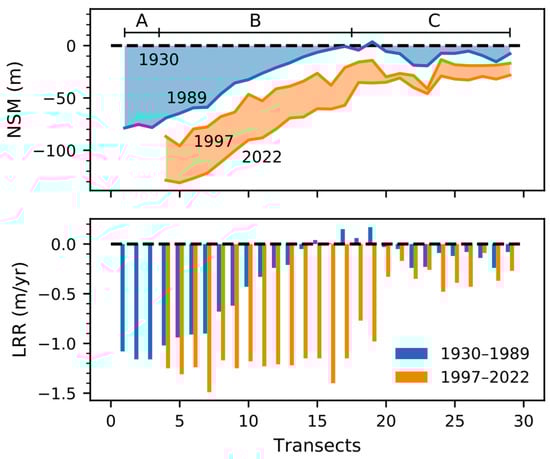
Figure 4.
The upper graph shows the NSM of all transects in zones A, B and C in the periods 1930–1989 and 1997–2022. The lower graph shows the LRR values of each transect for the same zones and periods.
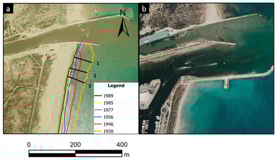
Figure 5.
(a) Shorelines and transects 1 to 3 from 1930 to 1989 (background image from 1989). (b) Image from 2022 of the same area.
In the northern area of zone B, near the breakwater (transects 4–8, Table 2 and Figure 6), the erosion during the period 1930–1989 is significant, with an average of 0.89 m/yr. It is worth remembering that between 1990 and 1992, the beach was regrown by about 50 m due to the creation of the marina [4]. As shown in Figure 4, this material added to the beach eroded rapidly, as the 1997 shoreline was behind the 1989 one. However, for the period 1997–2022, the values shot up to an average of 1.29 m/yr. It seems more than evident that the construction of the breakwater and the channelization of the river has accelerated a natural process (Figure 4). From transects 9 to 13, erosion rates only reach 0.36 m/yr for the period 1930–1989. This indicates that this zone, already farther from the mouth of the river, was less affected by the natural shoreline erosion. In contrast, after construction works in the area, the rate skyrockets to 1.22 m/yr, almost one meter more in a much shorter period of only 25 years. The erosion data for the area between transects 14 and 17 present a low LR2 for the first epoch analyzed. This is because the shorelines in this area are very close together, having accretion and erosion epochs, which makes it difficult to fit the linear regression [48]. In any case, the net movement of shoreline erosion in these transects was 5 m for the 60-year period (1930–1989). However, for the period 1997–2022, the mean NSM for these transects is 31.71 m, which seems to confirm the increase in erosion south of the breakwater. Looking at the entire period of 92 years, the mean erosion of all transects in zone B is 0.92 ± 0.24 m/yr. It happens that throughout zone B, erosion rates have increased after anthropic actions, reflecting their negative effects, especially in the southern part (Figure 4).
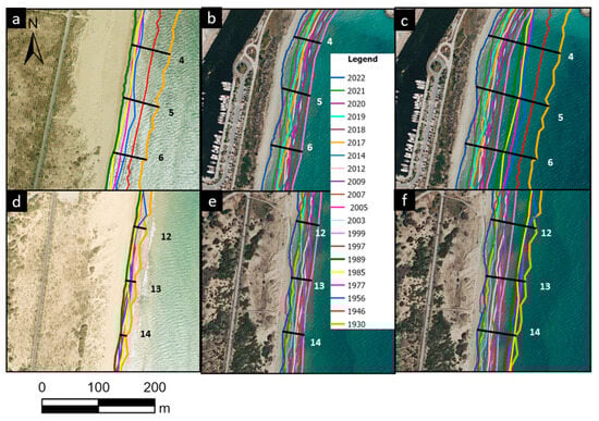
Figure 6.
Zone B. (a,d) Shorelines and transects from 1930 to 1989 (background image from 1989). (b,e) Shorelines and transects from 1997 to 2022 (background image from 2022). (c,f) Shorelines and transects from 1930 to 2022 (background image from 2022).
In zone C, for the period 1930–1989, something similar to zone B occurs with some of the linear regression, where the LR2 value is low. In this zone, some of the transects show a net accretion for this period (see Figure 4 and Figure 7a). Erosion at Babilonia Beach was very small until 1989, with only 8.72 m in 60 years, whereas in the last 25 years, 12.09 m, about 40% more, eroded in less than half the time. This has caused the loss of beaches in front of houses and, therefore, has left them directly exposed to sea waves (see Figure 2). However, as can be seen in Figure 7, the houses of Babilonia Beach act as an artificial barrier (or artificial shoreline), and therefore, there can be no further erosion except for the destruction of the houses themselves. If zone C is analyzed for the entire available time set, it can be observed that the fits are better and that the NSM value amounts to 33.86 m (0.32 m/yr). As in zone B, Figure 4 shows how erosion rates have increased after anthropogenic actions.
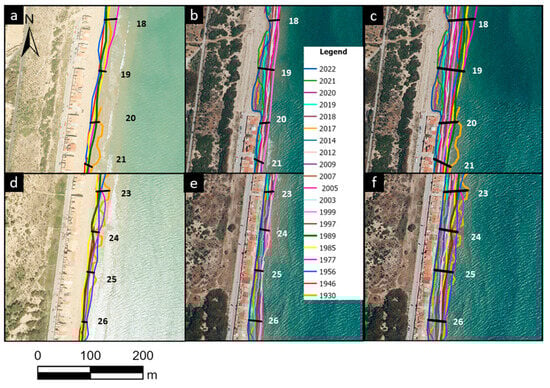
Figure 7.
Zone C. (a,d) Shorelines and transects from 1930 to 1989 (background image from 1989). (b,e) Shorelines and transects from 1997 to 2022 (background image from 2022). (c,f) Shorelines and transects from 1930 to 2022 (background image from 2022).
The effect of erosion on the houses of Babilonia Beach was also analyzed. During the 1930s and up to the 1970s, the built-up area increased, with 8533 m2 (55 houses) in 1930; 12,277 m2 (80 houses) in 1946; 17,976 m2 (117 houses) in 1956; and 19,463 m2 (126 houses) in 1977. This last value remained stable until 1999. From then on, and as a natural response to the values already discussed, the built-up area has been in continuous decline. Until 2005 the loss of floor area was a mere 131 m2 (one house). But from 2005 to 2012, the loss increased by 2218 m2 (14 houses) and has not stopped until 2022 (last data available), with a loss of another 1003 m2 (6 houses). One should consider the numerous attempts to protect these houses with the use of rock dikes, Hesco barriers filled with rock and sand, etc., that have managed to somewhat slow down the destruction of these houses [49].
Having historical erosion data in different transects, it is possible to apply the prediction models explained in Section 3.3. An adequate time horizon, preferably shorter than the available observation period (92 years), should be chosen to consider the data variability and, at the same time, to reduce the impact of data uncertainty on the quality of the results [39]. Therefore, the simulation is extended for 18 years, up to the year 2040 (see Table 3). Uncertainties have been incorporated for each model, including lower/upper bounds, having a surface area that delimits the possible solution (Figure 8). In the Lee–Clark model, uncertainty in the calculation of future erosion (LCe) is incorporated by adding (upper bound) and/or subtracting (lower bound) the LCI to the LRR value for each transect (see Table 2). For the Leatherman model, the limits are introduced using a minimum and maximum estimate of the rate of sea level rise in the future (S2). According to local estimates, the future rates will be a maximum (upper bound) of 0.5 mm/yr, with a reasonable minimum (lower bound) value of 0.25 mm/yr [25]. As mentioned in Section 2, the historical relative sea level rise (S1) has been 1.28 mm/yr.
Table 3.
Total shoreline erosion by 2040 in meters.
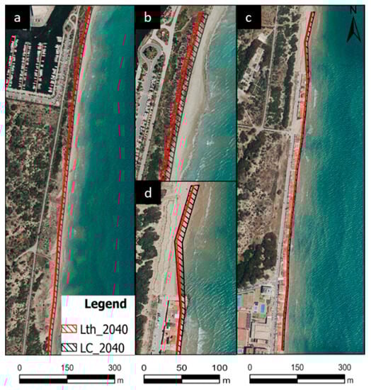
Figure 8.
Shoreline model predictions (Lth—Leatherman; LC—Lee and Clark) by year 2040: (a) general view of zone B; (b) detailed view of zone B; (c) detailed view of zone C; (d) general view for zone C.
As can be seen in Figure 8 and Table 3, the prediction models overlap in most cases. In this situation, it can be said that the shoreline is most likely to be located at some intersection surface of the two models. The Lee and Clark model has a larger difference between the lower and upper limits than the Leatherman. This is probably because the variability in historical erosion rates is greater than the effect of sea level changes for this relatively short simulation period. In the northern part of zone B, the shoreline is predicted to reach the area currently occupied by the cliff dune that, therefore, would also be eroded. In zone C, the houses continue to act as a barrier, although in the northern zone, erosion will increase and the loss of built-up area is likely to increase following the actual trend.
4.2. Cliff Dune Evolution (Past and Future)
The historical evolution of the cliff dune shows episodic erosion with major events between 2005 and 2007 and, more recently, between 2021 and 2022 (see Table 4 and Figure 9). In general, this is due to periods of major storms and an increase in wave height in the region [4,50]. In any case, the mean erosion value (including the 11 transects) for this area is 1.12 ± 0.66 m/yr. In this part of zone B, erosion data are 1.11 ± 0.20 m/yr for the period 1930–2022 and a little bit higher, 1.31 ± 0.77 m/yr, for the period 1999–2022. This shows, as is logical, that both cliff dunes and shorelines are closely related.
Table 4.
Erosion rates for profiles in zone D (cliff area) for the period: 1999-2022. Negative sign means erosion, while positive sign means accretion for NSM and LRR. Also, the total shoreline erosion with both models by 2040 in meters is shown.
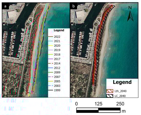
Figure 9.
(a) Cliff dune erosion since 1999, zone D. (b) Cliff dune erosion predictions (Lth—Leatherman; LC—Lee and Clark) by the year 2040.
The behavior of the Lee–Clark and Leatherman model prediction results are very similar to those obtained for the shoreline, with greater variability in the LC model and the Leatherman model mostly bordering the upper bound of the LC model. With both models, the prediction for the year 2040 is that erosion will be such that the paved road that parallels part of the marina will be eroded.
4.3. What Would Have Happened in the Area without Large-Scale Anthropogenic Actions?
With the data obtained in the previous sections, it is possible to simulate where the shoreline would be without the anthropic actions and compare it with the real situation. For this purpose, the Lee–Clark model is used in zones B and C for the pre-works period, i.e., from 1930 to 1989, as shown in Table 2.
In zone B (Figure 10), it can be seen how erosion has been advancing faster than natural erosion would have. This effect is especially noticeable in 2022 (Figure 10c,d), about 32 years after the start of the main works. At some points, such as transect 6, there was a difference of up to 10.85 m in 2005 (measured from the upper bound of the prediction to the shoreline), while in 2022, that difference increased to 20.85 m. However, this effect is felt more in the central sector of zone B; at transect 12, there was a difference of 23 m in 2005 and of 36 m in 2022. It appears evident that the effect of upstream constructions has accelerated the erosive process on the shoreline, especially in the central section of zone B (Figure 10b,d).
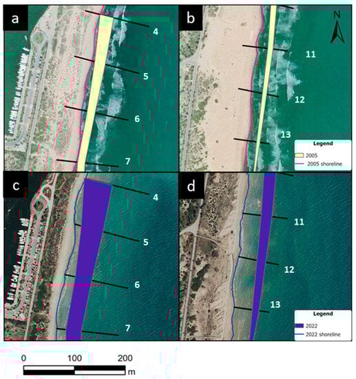
Figure 10.
Shoreline and area of possible erosion predicted with the LC model: (a) north of zone B by 2005; (b) middle sector of zone B by 2005; (c) north of zone B by 2022; (d) middle sector of zone B by 2022.
In Babilonia Beach, the erosion behavior is strongly conditioned by houses. An important characteristic in zone C is that in 2005 (Figure 11a,b), the houses had an important beach area that protected them from the direct action of the sea. In the 2022 images (Figure 11c,d), this beach does not exist anymore. Figure 11a,c show how a significant number of buildings have been destroyed from 2005 to 2022 and how these houses have been replaced by sand. This has left the way open for erosion, which has been increasing in contrast to what the model predicts (transect 19). According to the projections of the model used, erosion in some areas would have reached the housing area even without the works carried out, but these have undoubtedly had an important effect on the acceleration of this phenomenon.
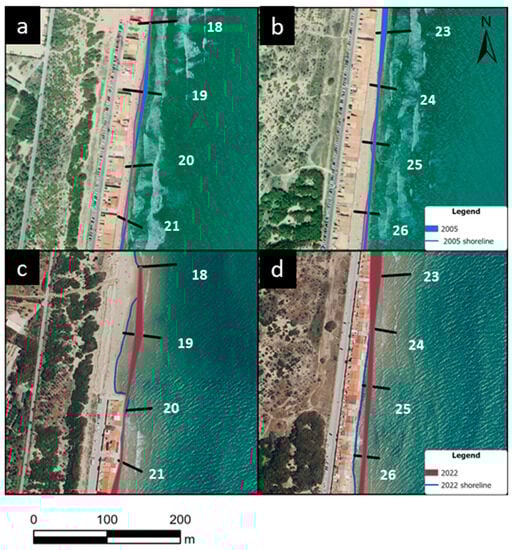
Figure 11.
Shoreline and area of possible erosion predicted with the LC model: (a) north of zone C by 2005; (b) middle sector of zone C by 2005; (c) north of zone C by 2022; (d) middle sector of zone C by 2022.
5. Conclusions
In general, the results presented and the methodology shown can be used to improve short- and medium-term decisions in areas where major construction is to be carried out, as well as where and when to intervene in coastal erosion processes. The conclusions in response to the objectives set out in the study are as follows:
- Erosion changes from one point of the coast to another and according to the period analyzed (1930–1989 or 1997–2022), which demonstrates the complex effect of anthropic actions that have accelerated the natural erosion of the area.
- The erosion of the cliff dune (zone D) shows episodic erosion due to strong storms but with rates in meters/year like those of the shoreline that protects it (zone B).
- The breakwaters at the mouth of the Segura River caused a loss of 3353 m2 of housing and an increment in shoreline erosion rates until 2022.
- The prediction models used overlap with each other; therefore, the predicted area would be the most likely for the shoreline situation in the year 2040. The Lee–Clark model (based on learning a model created on the derived dataset that is used for extrapolation of historical data) has greater variability than the Leatherman one (based on rates of sea level change), although the latter is always close to the maximum erosion limit of the former. In this area, the effect of the rate of sea level change does not seem to be very important in shoreline erosion since this value was already quite high during the last century.
- Comparing the actual shorelines in the years 2005 and 2022 with those simulated using the Lee–Clark model, it can be said that anthropogenic actions exhibit their effect by increasing erosion rates. This effect is more noticeable in the central zone of this study (southern part of zone B and northern part of zone C) and more limited in the marina zone (northern part of zone B) and in the houses on Babilonia Beach (southern part of zone C).
Author Contributions
Conceptualization, M.F.-H. and R.C.; methodology, A.C. and R.C.; software and data-based model learning, L.I., A.C. and A.J.D.-H.; validation, L.I., A.C. and M.F.-H.; formal analysis, R.C., J.J.O. and E.C.; investigation, M.F.-H., A.C. and P.M.; data curation, A.C. and L.I.; writing—original draft preparation, E.C., M.F.-H., R.C., J.J.O. and A.J.D.-H.; writing—review and editing, M.F.-H., A.C., L.I. and R.C.; visualization, A.C. and M.F.-H.; supervision, M.F.-H.; funding acquisition, R.C. All authors have read and agreed to the published version of the manuscript.
Funding
This work has been partially funded by the Universidad Politécnica de Madrid with grants to PDI and PhD researchers for international research stays of one month or more (resolution of 30 May 2022, of the Rector of the Universidad Politécnica de Madrid).
Institutional Review Board Statement
Not applicable.
Informed Consent Statement
Not applicable.
Data Availability Statement
The data presented in this study are available on request from the corresponding author. The data are not available to the public, as some of the images used must be requested from the Cartographic and Photographic Center of the Spanish Air Force and cannot be disseminated without permission.
Acknowledgments
The authors of this work would like to thank all the institutions that provide access to their material through official websites. The authors would like to thank the two anonymous reviewers for their contributions that have improved the final manuscript.
Conflicts of Interest
The authors declare no conflict of interest.
References
- Bio, A.; Gonçalves, J.A.; Iglesias, I.; Granja, H.; Pinho, J.; Bastos, L. Linking short-to medium-term beach dune dynamics to local features under wave and wind actions: A Northern Portuguese case study. Appl. Sci. 2022, 12, 4365. [Google Scholar] [CrossRef]
- Defeo, O.; McLachlan, A.; Armitage, D.; Elliott, M.; Pittman, J. Sandy beach social–ecological systems at risk: Regime shifts, collapses, and governance challenges. Front. Ecol. Environ. 2021, 19, 564–573. [Google Scholar] [CrossRef]
- United Nations. Available online: https://www.un.org/esa/sustdev/natlinfo/indicators/methodology_sheets/oceans_seas_coasts/pop_coastal_areas.pdf (accessed on 17 August 2023).
- Pagán, J.I.; López, I.; Aragonés, L.; Garcia-Barba, J. The effects of the anthropic actions on the sandy beaches of Guardamar del Segura, Spain. Sci. Total Environ. 2017, 601, 1364–1377. [Google Scholar] [CrossRef] [PubMed]
- Trenhaile, A.S. Climate change and its impact on rock coasts. Geol. Soc. Lond. Mem. 2014, 40, 7–17. [Google Scholar] [CrossRef]
- Syvitski, J.P.M.; Vörösmarty, C.J.; Kettner, A.J.; Green, P. Impact of humans on the flux of terrestrial sediment to the global coastal ocean. Science 2005, 308, 376–380. [Google Scholar] [CrossRef] [PubMed]
- Aragonés, L.; Pagán, J.I.; López, M.P.; García-Barba, J. 2016. The impacts of Segura River (Spain) channelization on the coastal seabed. Sci. Total Environ. 2016, 543, 493–504. [Google Scholar] [CrossRef]
- Biondo, M.; Buosi, C.; Trogu, D.; Mansfield, H.; Vacchi, M.; Ibba, A.; Porta, M.; Ruju, A.; De Muro, S. Natural vs. Anthropic Influence on the Multidecadal Shoreline Changes of Mediterranean Urban Beaches: Lessons from the Gulf of Cagliari (Sardinia). Water 2020, 12, 3578. [Google Scholar] [CrossRef]
- Anthony, E.J.; Almar, R.; Aagaard, T. Recent shoreline changes in the Volta River delta, West Africa: The roles of natural processes and human impacts. Afr. J. Aquat. Sci. 2016, 41, 81–87. [Google Scholar] [CrossRef]
- Villate, D.A.; Portz, L.; Manzolli, R.P.; Alcántara-Carrió, J. Human disturbances of shoreline morphodynamics and dune ecosystem at the Puerto Velero spit (Colombian Caribbean). J. Coast. Res. 2020, 95, 711–716. [Google Scholar] [CrossRef]
- de Schipper, M.A.; Ludka, B.C.; Raubenheimer, B.; Luijendijk, A.P.; Schlacher, T.A. Beach nourishment has complex implications for the future of sandy shores. Nat. Rev. Earth Environ. 2021, 2, 70–84. [Google Scholar] [CrossRef]
- Lee, J.T.; Shih, C.Y.; Hsu, Y.S. Root biomechanical features and wind erosion resistance of three native leguminous psammophytes for coastal dune restoration. Ecol. Eng. 2023, 191, 106966. [Google Scholar] [CrossRef]
- Franco-Ochoa, C.; Zambrano-Medina, Y.; Plata-Rocha, W.; Monjardín-Armenta, S.; Rodríguez-Cueto, Y.; Escudero, M.; Mendoza, E. Long-term analysis of wave climate and shoreline change along the Gulf of California. Appl. Sci. 2020, 10, 8719. [Google Scholar] [CrossRef]
- Yum, S.G.; Park, S.; Lee, J.J.; Adhikari, M.D. A quantitative analysis of multi-decadal shoreline changes along the East Coast of South Korea. Sci. Total Environ. 2023, 876, 162756. [Google Scholar] [CrossRef] [PubMed]
- Skilodimou, H.D.; Antoniou, V.; Bathrellos, G.D.; Tsami, E. Mapping of coastline changes in Athens Riviera over the past 76 year’s measurements. Water 2021, 13, 2135. [Google Scholar] [CrossRef]
- Griggs, G.; Reguero, B.G. Coastal adaptation to climate change and sea-level rise. Water 2021, 13, 2151. [Google Scholar] [CrossRef]
- Zhu, X.; Linham, M.M.; Nicholls, R.J. Technologies for Climate Change Adaptation. Coastal Erosion and Flooding, 1st ed.; UNEP Risø Centre on Energy, Climate and Sustainable Development: Roskilde, Denmark, 2010. [Google Scholar]
- Bacopoulos, P.; Clark, R.R. Coastal erosion and structural damage due to four consecutive-year major hurricanes: Beach projects afford resilience and coastal protection. Ocean. Coast. Manag. 2021, 209, 105643. [Google Scholar] [CrossRef]
- Simeone, S.; Palombo, L.; Molinaroli, E.; Brambilla, W.; Conforti, A.; De Falco, G. Shoreline response to wave forcing and sea level rise along a geomorphological complex coastline (western Sardinia, Mediterranean Sea). Appl. Sci. 2021, 11, 4009. [Google Scholar] [CrossRef]
- Pagán, J.I.; López, M.; López, I.; Tenza-Abril, A.J.; Aragonés, L. Causes of the different behaviour of the shoreline on beaches with similar characteristics. Study case of the San Juan and Guardamar del Segura beaches, Spain. Sci. Total Environ. 2018, 634, 739–748. [Google Scholar] [CrossRef]
- Puertos del Estado. Available online: https://www.puertos.es/es-ES/Paginas/avisolegal.aspx (accessed on 5 June 2023).
- Martí Talavera, J.; Amor Jiménez, J.A.; Giménez García, R.; Ruiz Álvarez, V.; Biener Camacho, S. Episodio de lluvias torrenciales del 11 al 15 de septiembre de 2019 en el sureste de la Península Ibérica: Análisis meteorológico y consecuencias de las transformaciones en los usos del suelo. Finisterra 2021, 56, 151–174. [Google Scholar] [CrossRef]
- Ali, E.; Cramer, W.; Carnicer, J.; Georgopoulou, E.; Hilmi, N.J.M.; Le Cozannet, G.; Lionello, P. Cross-Chapter Paper 4: Mediterranean Region. In Climate Change 2022: Impacts, Adaptation and Vulnerability. Contribution of Working Group II to the Sixth Assessment Report of the Intergovernmental Panel on Climate Change, 1st ed.; Pörtner, H.O., Roberts, D.C., Tignor, M., Poloczanska, E.S., Mintenbeck, K., Alegría, A., Craig, M., Langsdorf, S., Löschke, S., Möller, V., et al., Eds.; Cambridge University Press: Cambridge, UK; New York, NY, USA, 2022; pp. 2233–2272. [Google Scholar] [CrossRef]
- Wöppelmann, G.; Marcos, M. Coastal Sea level rise in southern Europe and the nonclimate contribution of vertical land motion. J. Geophys. Res. 2012, 117, C01007. [Google Scholar] [CrossRef]
- Zerbini, S.; Raicich, F.; Prati, C.M.; Bruni, S.; Del Conte, S.; Errico, M.; Santi, E. Sea-level change in the Northern Mediterranean Sea from long-period tide gauge time series. Earth-Sci. Rev. 2017, 167, 72–87. [Google Scholar] [CrossRef]
- Alfosea, F.J.T.; Cantos, J.O. Incidencia de los temporales de levante en la ordenación del litoral alicantino. Papeles Geogr. 1997, 26, 105–132. [Google Scholar]
- CHS—Confederación Hidrográfica del Segura. Available online: https://www.chsegura.es/es/ (accessed on 8 June 2023).
- Matarredona Coll, E.; Marco Molina, J.A.; Prieto Cerdán, A. La configuración física del litoral sur alicantino. In Guía de Campo de las XXI Jornadas de Geografía Física, 1st ed.; Giménez-Font, P., Marco-Molina, J.A., Matarredona-Coll, E., Padilla-Blanco, A., Sánchez-Pardo, A., Eds.; Universitat d’Alacant, Instituto Universitario de Geografía: Alicante, Spain, 2006; pp. 35–47. [Google Scholar]
- MAPAMA. Recuperación del Ecosistema Dunar de Guardamar del Segura, Tramo Casas de Babilonia—Desembocadura del río Segura, Alicante; Costas, D.G.D., Ed.; Ministerio de Agricultura, Pesca y Alimentación: Madrid, Spain, 2001.
- Pagán, J.I.; Bañón, L.; López, I.; Bañón, C.; Aragonés, L. Monitoring the dune-beach system of Guardamar del Segura (Spain) using UAV, SfM and GIS techniques. Sci. Total Environ. 2019, 687, 1034–1045. [Google Scholar] [CrossRef] [PubMed]
- Himmelstoss, E.A.; Henderson, R.E.; Kratzmann, M.G.; Farris, A.S. Digital Shoreline Analysis System (DSAS) Version 5.1 User Guide: U.S. Geological Survey Open-File Report 2021–1091; U.S. Geological Survey: Reston, VA, USA, 2021; p. 104. [CrossRef]
- Centro de Descargas—Centro Nacional de Información Geográfica. Available online: https://centrodedescargas.cnig.es/CentroDescargas/index.jsp (accessed on 8 February 2023).
- Institut Cartogràfic Valencià. Available online: https://icv.gva.es/es/ (accessed on 14 February 2023).
- AgiSoft PhotoScan Professional. Available online: http://www.agisoft.com/downloads/installer/ (accessed on 2 February 2023).
- Longley, P.A.; Goodchild, M.F.; Maguire, D.J.; Rhind, D.W. Geographic Information Science and Systems, 4th ed.; John Wiley & Sons, Ltd.: Chichester, England, 2015; p. 480. [Google Scholar]
- Tsiakos, C.A.D.; Chalkias, C. Use of Machine Learning and Remote Sensing Techniques for Shoreline Monitoring: A Review of Recent Literature. Appl. Sci. 2023, 13, 3268. [Google Scholar] [CrossRef]
- Ojeda Zújar, J.; Fernández Núñez, M.; Prieto Campos, A.; Pérez Alcántara, J.P.; Vallejo Villalta, I. Levantamiento de líneas de costa a escalas de detalle para el litoral de Andalucía: Criterios, modelo de datos y explotación. In Tecnologías de la Información Geográfica: La Información Geográfica al Servicio de los Ciudadanos, 1st ed.; Ojeda, J., Pita, M.F., Vallejo, I., Eds.; Secretariado de Publicaciones de la Universidad de Sevilla: Seville, Spain, 2010; pp. 324–336. [Google Scholar]
- Pagán, J.I.; Aragonés, L.; Tenza-Abril, A.J.; Pallarés, P. The influence of anthropic actions on the evolution of an urban beach: Case study of Marineta Cassiana beach, Spain. Sci. Total Environ. 2016, 559, 242–255. [Google Scholar] [CrossRef]
- Castedo, R.; de la Vega-Panizo, R.; Fernández-Hernández, M.; Paredes, C. Measurement of historical cliff-top changes and estimation of future trends using GIS data between Bridlington and Hornsea–Holderness Coast (UK). Geomorphology 2015, 230, 146–160. [Google Scholar] [CrossRef]
- Sede Electrónica del Catastro. Available online: https://www.sedecatastro.gob.es/ (accessed on 23 March 2023).
- Islam, M.S.; Crawford, T.W. Assessment of spatio-temporal empirical forecasting performance of future shoreline positions. Remote Sen. 2022, 14, 6364. [Google Scholar] [CrossRef]
- Farris, A.S.; Long, J.W.; Himmelstoss, E.A. Accuracy of shoreline forecasting using sparse data. Ocean Coast. Manag. 2023, 239, 106621. [Google Scholar] [CrossRef]
- Lee, E.M.; Clark, A.R. Investigation and Management of Soft Rock Cliffs; Thomas Telford: London, UK, 2002. [Google Scholar]
- Castedo, R.; Paredes, C.; de la Vega-Panizo, R.; Santos, A.P. The modelling of coastal cliffs and future trends. In Hydro-Geomorphology–Models and Trends, 2nd ed.; Shukla, D.P., Ed.; IntechOpen: Rijeka, Croatia, 2017; pp. 53–78. [Google Scholar]
- Leatherman, S.P. Modeling shore response to sea-level rise on sedimentary coasts. Prog. Phys. Geogr. 1990, 14, 447–464. [Google Scholar] [CrossRef]
- Athanasiou, P.; van Dongeren, A.; Giardino, A.; Vousdoukas, M.I.; Ranasinghe, R.; Kwadijk, J. Uncertainties in projections of sandy beach erosion due to sea level rise: An analysis at the European scale. Sci. Rep. 2020, 10, 11895. [Google Scholar] [CrossRef]
- Bagheri, M.; Ibrahim, Z.Z.; Mansor, S.; Abd Manaf, L.; Akhir, M.F.; Talaat, W.I.A.W.; Wolf, I.D. Hazard Assessment and Modeling of Erosion and Sea Level Rise under Global Climate Change Conditions for Coastal City Management. Nat. Hazards Rev. 2023, 24, 04022038. [Google Scholar] [CrossRef]
- Frost, J. Regression Analysis: An Intuitive Guide for Using and Interpreting Linear Models, 1st ed.; Jim Publishing: Pennsylvania, PA, USA, 2020; p. 355. [Google Scholar]
- NIUS Diario. Available online: https://www.niusdiario.es/espana/valencia/20230406/colonia-babilonia-playa-ruinas-guardamar-segura_18_09202722.html (accessed on 29 June 2023).
- Oliva Cañizares, A.; Olcina, J. Temporales marítimos, cambio climático y cartografía de detalle de ocupación de la franja costera: Diagnóstico en el sur de la provincia de Alicante (España). Doc. D’anàlisi Geogràfica 2022, 68, 107–138. [Google Scholar] [CrossRef]
Disclaimer/Publisher’s Note: The statements, opinions and data contained in all publications are solely those of the individual author(s) and contributor(s) and not of MDPI and/or the editor(s). MDPI and/or the editor(s) disclaim responsibility for any injury to people or property resulting from any ideas, methods, instructions or products referred to in the content. |
© 2023 by the authors. Licensee MDPI, Basel, Switzerland. This article is an open access article distributed under the terms and conditions of the Creative Commons Attribution (CC BY) license (https://creativecommons.org/licenses/by/4.0/).