Abstract
In order to find optimized headlight distributions based on real traffic data, a three-step approach has been chosen. The complete investigations are too extensive to fit into a single paper; this paper is the last of a three part series. Over the three papers, a novel way to optimize automotive headlight distributions based on real-life traffic and eye tracking data is presented. Across all three papers, a total of 119 test subjects participated in the studies with over 15,000 km of driving, including recordings of gaze behaviour, light data, detection distances, and other objects in traffic. In this third paper, driver gaze behaviour is recorded while driving a 128 km round course, covering urban roads, country roads, and motorways. This gaze behaviour is then analysed and compared to prior work covering driver gaze behaviour. Comparing the gaze distributions with roadway object distributions from part two of this series, Analysis of Real-World Traffic Data in Germany and combining them with the idealized baseline headlight distribution from part one, different optimized headlight distributions can be generated. These headlight distributions can be optimized for different driving requirements based on the data that is used and weighting the different road types differently. The resulting headlight distribution is then compared to a standard light distribution in terms of the required luminous flux, angular distribution, and overall shape. Nonetheless, it is the overall approach that has been taken that we see as the primary novel outcome of this investigation, even more than the actual distribution resulting from this effort.
1. Introduction
When investigating the light levels and distributions required for safe nighttime driving, analysing the gaze behaviour of a driver is a useful step, as most of the information gathered by drivers is obtained visually [1]. Since the science of tracking drivers’ gaze behaviour has been evolving since at least 1972 [2], much work has been published over the last 50 years. In recent years, there have been numerous investigations into visibility from advanced headlighting systems and on the illumination requirements for visually guided behaviour [3,4,5,6,7,8,9,10,11,12,13]. Many different topics have been investigated such as the difference of gaze orientation between experienced and inexperienced drivers [2], orientation behaviour when cornering [14], and gaze directions of tired versus vigilant drivers [15]. With the introduction of new headlamp systems, the influence of different lighting systems on gaze behaviour was also studied extensively.
Damasky, Brückman, Diem, Schulz, Winter, and Shibata all investigated the influence of different headlight systems on the gaze behaviour of drivers [16,17,18,19,20,21,22], albeit to address different research questions. The approach of Diem comes closest to the approach chosen in this paper series. In his studies, the overall gaze behaviour in real-life traffic situations was recorded. The data were then split into different overall categories and the data acquired in these categories were compared to the data acquired in similar situations, but during the daytime.
While a substantial amount of research has been conducted on this very topic of gaze behaviour during the night, it is crucial for this paper’s approach to conduct new studies. One reason is that the technology available for gaze tracking has improved drastically, with new camera technologies allowing for high-resolution capture of the driver’s eyes, and much increased computational power allowing for the evaluation of large datasets in a much shorter time (Diem for example evaluated his data manually on video). Another reason is that new data that are recorded simultaneously with video data of the road are needed for the current study’s approach. The gaze behaviour acquired in this study will be compared with the data presented in part two of this series, Analysis of Real-World Traffic Data in Germany, where roadway object distributions in real traffic situations were recorded. Since the gaze behaviour was recorded simultaneously with the object data, both distributions can be compared directly, showing not only where drivers look but what they look at while driving. Knowing the exact light distribution of the test vehicle and the data published by Diem, Brückmann, and Damasky, assumptions can be made on how different light distributions could affect the gaze behaviour. Combining all of these data, a newly optimized light distribution is derived in this series of papers.
2. Driver Gaze Behaviour on Real Roads
This first section will cover the required test set-up, give an overview of the test procedure including the calibration routine, describe the test subjects in more detail, and show examples of the acquired gaze data, as well as providing a short comparison to existing work. The comparison to existing work is mainly for validation purposes and to show that the system as implemented works as intended.
2.1. Test Vehicle
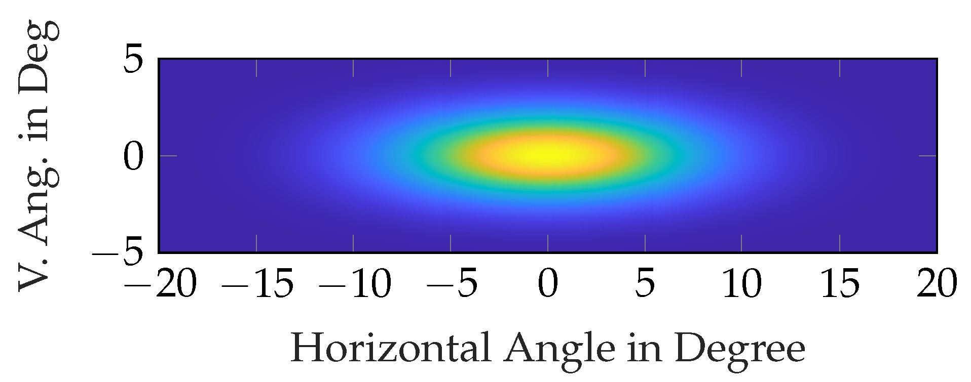
The test vehicle used in this test, is the same vehicle that was used in part two, Analysis of Real-World Traffic Data in Germany, as the data for both parts were recorded simultaneously. Additionally to the set-up previously described, an eye tracking camera system consisting of four cameras pointing towards the driver was used. Since the headlights and especially the light distribution is important for this part of the paper series, the passing (low) beam light distribution of the light emitting diode (LED) headlights on this vehicle is shown in Figure 1.
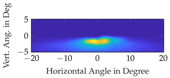
Figure 1.
Light distribution of the BMW 3 Series passing (low) beam as used in this study. In the false colour representation shown, the darker blues correspond to lower intensities, while the lighter yellows correspond to higher intensities.
2.1.1. Eye Tracking System
The eye tracking system that was used is a Smart Eye system. This system records all head and eye movement of the driver at 120 . A time stamp is added to these data to synchronize the gaze data with the data shown in the second paper of our series. The four cameras are mounted to the chassis of the test vehicle using custom aluminium stands to minimize the movement of the cameras and to ensure that the relative positions, including rotations, between the cameras does not change over the course of a test drive. The cameras use an infrared filter so that the exposure is kept constant under different exterior light conditions. For this reason, three infrared light sources were placed between the cameras. The driver’s view can be seen in Figure 2, where the equipment used for the tests from part two is also shown.
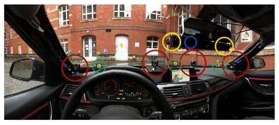
Figure 2.
Interior of the test vehicle, with the eye tracking cameras marked by red circles, the infrared LEDs for illumination marked by green circles, the stereo camera used for part two of this series marked in yellow, and an illuminance sensor marked by the blue circle.
2.1.2. GPS and Light Measurement
As shown in Figure 2, additionally, an illuminance sensor was placed behind the rear view mirror. This sensor was placed in a position where it did not interfere with the vision of the driver, while at the same time being placed as closely as possible to the driver’s head position to measure the illuminance at the driver’s eye. The system was a Gigahertz Electronics X1, measuring at 20 . Additionally, a GPS sensor, measuring at 10 , was set up outside of the car to measure the driving speed and to control the route, as described in part two of this paper series.
2.2. Test Procedure
Since an eye tracking system requires intensive calibration routines, this section will explain the complete procedure performed for each test drive.
2.2.1. Calibration
In the first step, the eye tracking cameras need to be calibrated with each other in order to calculate the distance and the relative movement of the driver’s head and from that, the eye movement. For this, a chequerboard pattern was presented to all four cameras at the same time. From the relative distortion of the pattern, the individual orientations of all cameras were calculated automatically by the Smart Eye system.
In the next step, the test subject is invited to the vehicle and the calibration of the system to the driver is performed. This step is necessary since the eye tracking system itself is only able to calculate a vector from the centre of the eyeball through the pupil’s centre. However, the gaze vector of each individual is slightly different from this measured vector. Thus, an individual calibration that calculates the difference between these two vectors is necessary.
For this study, a six point calibration is performed. For this, each test subject is asked to look at a series of six fixed markers. The position of these markers relative to the coordinate system of the cameras inside of the car is known. By this information the calculated vector by the system can be corrected to match the chosen vectors for the calibration. Since this calibration has some uncertainty, and each individual has a wide variety of unconscious eye movements [23,24,25], the measured data will always exhibit scattering around the targets even after calibration. From these data, two major metrics are derived: the accuracy, showing how much the mean gaze vector deviated from the theoretical gaze vector, and the precision, showing how much the gaze vector scattered around the mean gaze vector.
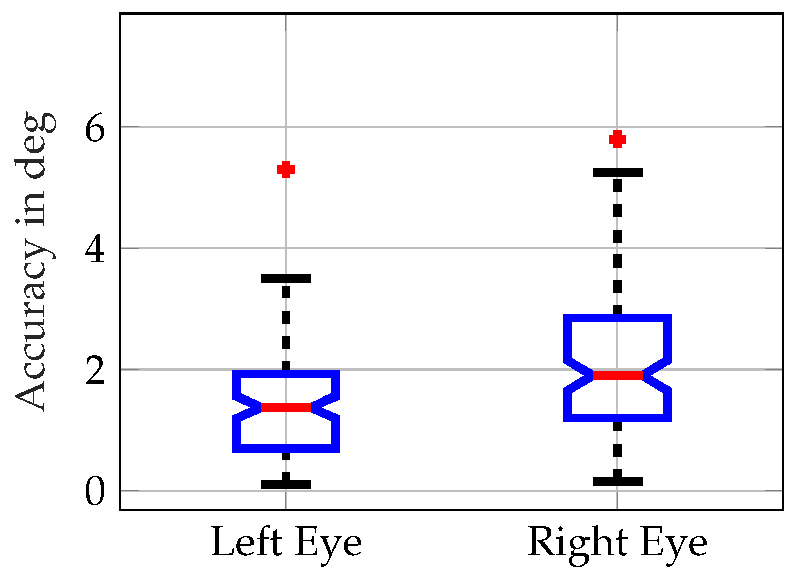
To achieve reasonable results, only test subjects with both accuracy and precision below were chosen for the study. The accuracy and the precision data for all test subjects, separated for each eye individually, are shown in Figure 3 for accuracy and in Figure 4 for precision.
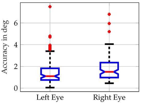
Figure 3.
Accuracy for all 54 test subjects divided by left and right eyes after the calibration: shown as a box plot with the median (red line), the 25% and 75% quartiles (blue boxes), the whiskers (dashed black lines), and the outliers (red diamonds).
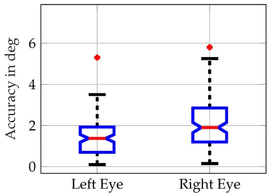
Figure 4.
Precision for all 54 test subjects divided by left and right eye after calibration: shown as a box plot with the median (red line), the 25% and 75% quartiles (blue boxes), the whiskers (dashed black lines), and the outliers (red diamonds).
The accuracy data clearly show that, overall, accuracy is best for the left eye and that a mean accuracy of around one degree is achieved with this system.
Similar findings can be made when it comes to precision. Again, on average the left eye shows the better results, with a mean precision of about .
Since accuracy and precision were different for each eye, for each test subject, the more accurate eye was chosen for the gaze data.
2.2.2. Test Subjects
As mentioned above, a total of 54 test subjects participated in this study. After selecting only subjects with both accuracy and precision below , only 15 of the initial 54 test subjects remained for further evaluation. It should be remarked here, that due to the relatively long preparation time and the different parameters used in addition to gaze tracking, the complete test was conducted with all 54 test subjects; only the analysis of gaze behaviour was limited to these 15 subjects.
All of the test subjects were between 20 and 40 years of age. Every subject had had a driver’s licence for at least one year and drove a minimum of 1000 km per year. From the 54 subjects, 16 were female. From the 15 subjects with both accuracy and precision of gaze tracking below , 2 were female. All test subjects were asked to wear their appropriate corrective lenses for driving (if any) and to arrive at the test location well rested. To test their attention span, a memory test was performed before and after the test drive. Overall, no significant change in the attention span of the subjects was recorded after the test drive.
2.2.3. Route
The route driven is identical to the route used to measure traffic conditions in the second paper of this series, since the data were acquired simultaneously to that data collection effort. To summarize, the total route is 128 km, consisting in roughly equal parts of motorways, rural roads, and urban roads around Darmstadt and Frankfurt.
2.2.4. Driving Conditions
As previous studies have shown, gaze behaviour is highly dependent on different environmental conditions such as speed, time of day, and light conditions. The illuminance sensor was placed behind the rear view mirror to measure incoming light at the driver’s eye. For the test runs, the average illuminance values for urban roads were , for rural roads were , and for motorways were . The complete data for all three road categories are displayed in Figure 5. All nighttime test drives started at the same time (19:00 p.m.) and were only conducted during weekdays to ensure similar traffic situations for all drivers. Test drives were only conducted on days with dry weather.
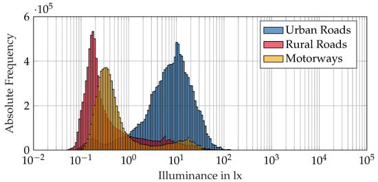
Figure 5.
Illuminance values recorded during the nighttime drives for urban roads (blue), rural roads (red), and motorways (yellow).
This figure shows that the illuminance while driving through cities is substantially higher than along rural roads and motorways. This is likely due to additional fixed road lighting, more frequent oncoming traffic, and illuminated advertisement and store fronts that cannot be found along the other categories of roads.
For driving speeds, the recorded average driving speed on urban roads was km , km on rural roads, and km on motorways. For the calculation of these data, only data points with a speed of above 1 km were used, meaning that traffic jams and waiting at traffic lights were excluded. The reason for this is that during those situations an optimization of light distributions is unnecessary and recording the gaze data during these standing periods would lead to skewed distributions since drivers would not need to focus on the road during those times.
2.3. Results
In order to visualize the gaze distributions, several calculations were required. Since the starting point of each gaze vector is each subject’s eye with the greatest accuracy and precision, and since the head of each test subject is located at a different position depending on body size and seat position, and also moves around while driving, the origin of each gaze vector is moving throughout the data collection. For that reason, displaying gaze angles only, horizontal and vertical, does not lead to valid results.
In order to obtain valid results, each single gaze vector is intersected with a plane at a distance of 25 away from the test vehicle’s windscreen. Obviously, changing the distance of this plane would change the gaze distribution. However, testing this for 25, 50, and 75 m showed only minimal changes in the distribution. However, changing the distance of this intersecting plane down to 1 changes the distributions quite drastically, since the head position now influences the gaze vectors significantly.
2.3.1. Gaze Distributions during Night
Looking at the overall gaze distributions did not lead to any new findings. Therefore, this section will only show selected situations and road categories. Furthermore, investigating the overall gaze data did not necessarily lead to the desired insight since a large portion of these recorded gaze vectors were just scanning gazes not leading to any information gathering for the driver. For this reason, the data presented here focus solely on fixations. For this paper, a fixation is defined as a gaze direction that stays within a area for more than 200 ms [26]. The area is, for this evaluation, set to be around the moving mean value of the last 50 ms to ensure that the behaviour of tracking objects will be evaluated as well [27,28].
One important remark here is that from the overall collected gaze dataset, 24.4% of the data are correlated to fixations during the night, while only 18.3% of the daytime data are correlated to fixations. This indicates that the additional light available during the day may lead to more scanning gaze behaviour, while the limited light available during the night leads to a more fixation-oriented gaze behaviour.
While the overall fixation distribution did not lead to any particular insight, the most important metrics are given in Table 1. As a comparison, the same data are presented for the daytime driving. Additionally to the median values, the standard deviation of both the horizontal and vertical fixations as well as the median fixation distances, where the fixation vectors intersect with the road surface, are given.

Table 1.
Fixation data for daytime and nighttime driving. The distance d is calculated as the intersection of the fixation vectors with the road surfaces.
Without going into too much detail, the difference between the fixation distributions between daytime and nighttime driving mainly appears to be the gaze distance (), which is more than double the distance during the day. The nighttime fixation distributions also appear to be slightly narrower than the overall daytime distribution.
Both of these effects are to be expected due to the limited amount of light available during the nighttime. Without going into more detail about the daytime fixations, Table 2 shows the same information for nighttime driving, but divided into the three major road categories.
Table 2.
Fixation data for the different road categories during nighttime driving.
The data shows, when compared to the average speed that is being driven in each of these road categories, that the orientation distance is highly speed dependent. The higher the speed, the higher and smaller the fixation areas are. The relatively far distance of 229 for highway driving is mainly due to the focus on preceding vehicles, and not on the road ahead. Therefore, while the fixation vectors might intersect the road 229 ahead of the driver, the actual fixation, in terms of other vehicles, could be much closer. However, an exact distance cannot be derived from this analysis.
2.3.2. Comparison to Previous Work
Three main points are described here when comparing to the gaze distributions reported in previous studies. First of all, the finding that during the night gaze distributions become narrower and closer to the vehicles was already found by Brückmann and Diem [17,18]; Damasky, however, has found the exact opposite [16]. The difference in fixation behaviour on different road types, however, match the results presented by Diem.
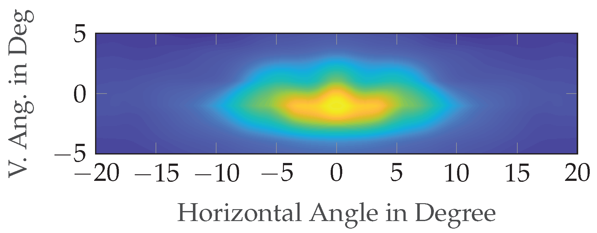
Additionally, to further verify the data acquired for this study, the data were compared to the orientation behaviour found by Shibata [19]. For this, curves with similar radii to those of Shibata’s study, 150 to 250 were selected. The datasets from this study as well as the data from Shibata are shown in Figure 6, and they clearly show that a very similar orientation behaviour is found. The data acquired in this study is colour-graded, with dark blue areas showing no fixations and yellow showing the normalized maximum of the recorded fixations. Shibata’s data are marked by red crosses, and in black lines a curve with a 200 radius is inserted into the graphic as well.
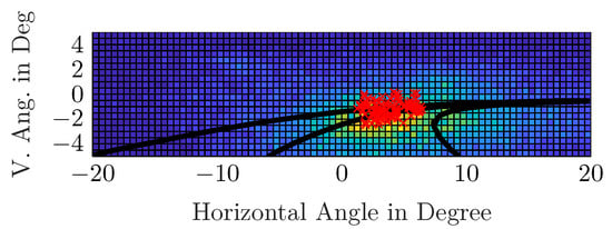
Figure 6.
Fixation data while driving through curves with a radius between 150 and 250 . Data digitalized from Shibata [19] are marked by red crosses. In the false colour representation shown, the darker blues correspond to low fixation numbers, while the lighter yellows correspond to higher fixation numbers.
All of these findings mainly show that the eye tracking system works as intended and that the chosen route represents, at least from a gaze behaviour point of view, a representative road system. The next step is, therefore, to use the present data to develop an optimized light distribution.
3. Optimizing Light Distributions
In this section, the data acquired from the studies in all three papers in this series will be brought together to achieve a simple, optimized light distribution. As a starting point, the gaze data acquired in this part of the paper series are taken and compared to the object data from part two, Analysis of Real-World Traffic Data in Germany.
The main concept is that areas that are shown to contain many “important” traffic objects, such as other cars, pedestrians, or cyclists, should receive a lot of “attention”, which in this study is represented by fixations. Areas in which no such objects appear do not require fixations from the driver.
To make the comparison, the normalized mean fixation distribution is subtracted from the normalized mean object distribution. With both distributions being normalized to their corresponding maximum, both data matrices have a minimum value of 0 and a maximum value of 1, meaning that the resulting modification matrix (Figure 7) has a minimum of −1 for areas where only gazes but no objects were detected, 0 where equal amounts of objects and gazes were measured, and +1 where only objects and no fixations were found. This is visualized in Figure 7. Orange and yellow areas mark those areas in which more objects than fixations are recorded (positive values). Green areas show those parts in which roughly equal amounts of fixations and objects are found (values around 0) and blue areas show the parts in which more fixations than objects are detected (negative values).
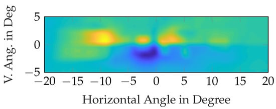
Figure 7.
Visual representation of the modification matrix that was calculated by subtracting the normalized fixation data from the normalized object distributions. Yellow areas represent more objects than fixations and blue areas mark the opposite. Green areas show where roughly the same amount of gazes and objects were found.
For the next step, the base light distribution from part one, Idealized Baseline Headlight Distribution, shown in Figure 8, is taken into account as well. As described in part one of this series, this headlight distribution was determined from detection tests under different horizontal angles under ideal conditions for the driver, including a completely straight road, no other traffic participants, no other lighting than the vehicle’s headlights, and only one detection object that was placed along different detection angles.

Figure 8.
Baseline headlight distribution used as a starting point for the optimization of the headlight distribution in the present study.
Multiplying the matrices represented by Figure 7 and Figure 8, results in a matrix that takes the baseline light that is required to detect objects under certain angles and modifies it according to the frequency of both fixations and objects found in real-life traffic. Since the resulting light distribution, as evident from Figure 7, is not going to be symmetrical and will have some hotspots, the result will be mirrored and smoothed in both the vertical and horizontal directions by a moving mean smoothing filter over 10 values corresponding to in order to generate a light distribution that fits for right-hand traffic as well as for left-hand traffic. The result of this is displayed in Figure 9.

Figure 9.
Mirrored and smoothed proposed new headlight distribution based on real traffic and gaze data as well as on detection tests under ideal road conditions.
The resulting headlight distribution can be rather clearly separated into two areas. Below 0 vertically, a wide area is illuminated. Above the horizon, only a small “hotspot” is visible. This is rather similar to current light distributions, with a wide passing beam and a narrow but bright main beam.
If the data acquired in part one, Idealized Baseline Headlight Distribution, for the luminous intensity is used here for scaling the intensity of the centre hotspot, the total luminous flux as well as the width of this light distribution can be compared to current headlamps. For this example, the generated light distribution is compared to the light distribution of the test vehicle used in the detection studies, as presented in Figure 1, with added high beam.
This leads to an increase in the total luminous flux of about 66%, mainly coming from the much wider distribution in the high beam area. For example, 50% of the maximum is reached at for the proposed headlight distribution, while the headlight distribution from the test vehicle reaches the 50% already at from the centre. Furthermore, the decrease in intensity when comparing the passing beam part of the headlight with the main beam part of the headlamp is not as strong for the proposed light distribution. The maximum at vertically is around 20% higher for the proposed headlight distribution.
Overall, this optimized headlight distribution mimics currently available high-end light distributions rather similarly. The differences in width and intensity are rather small; however, the increase in total luminous flux of 66% is significant.
4. Discussion
When looking only at the third part of this three part paper series, it might seem that only using 15 test subjects for the gaze analysis seems like a small number of test subjects, especially considering that a total of 54 test subjects participated in the study presented here. However, using 15 test subjects with an average of over each and a sample rate of 120 for the eye tracking system led to a total of more than 900 million gaze vectors that had to be analysed for the nighttime driving alone. Nonetheless, it is the analytical approach embodied in this and earlier papers that is the main novel outcome of the present work, more so than the resulting headlight distribution. For this reason, the decision to only evaluate the data test subjects with calibration results below , would be expected to influence the acquired results positively rather than negatively.
However, one major point needs to be addressed. All of the data shown in this part, as well as in part two, were acquired on the same single route through Germany. So, while the data, when compared to similar data found by other studies, seems similar and by that representative of overall road conditions, it cannot truly be representative for the world, for Europe, or even for Germany. Therefore, the proposed light distribution is to be taken with the required scepticism. A more appropriate approach would be to consider this paper as a starting point and as a novel way to create an optimized headlight distribution.
On the same note, it should be noted, that the light distribution shown in Figure 9 has been created by simply using all the available data for urban roads, rural roads, and motorways and weighting them all equally. Obviously different cars are created with different driving types in mind. Small cars that are mainly designed to be driven inside of large cities, for example, could use a different light distribution than cars that are typically designed for longer journeys, and which will be mainly driven on motorways.
Additionally, with the current technology and increasing possibilities of those technologies in modern headlights, a scenario is possible where thousands of different light distributions could be programmed into a single headlamp. Then, the next step would be to go through datasets such as the ones created for the present studies, and to define more granular situations in which different light distributions might increase traffic safety. Following this, the light distributions for those different situations could be optimized.
The three-part approach taken in this and the accompanying papers (parts one and two) illustrate how it might be possible to use empirical visual detection data from closed-road investigations and apply the resulting photometric requirements to real-world roadway environments such as the ones underlying the test drives in this and the previous papers. Of course, the data and real-world environments are limited in the current study. As a result, this paper should be considered as a starting point for future research rather than a definitive optimized headlight distribution.
Author Contributions
Conceptualization, J.K.; data curation, J.K.; formal analysis, J.K.; methodology, J.K.; software, J.K.; supervision, T.Q.K.; validation, J.K.; visualization, J.K. and A.E.; writing—original draft, J.K. and A.E.; writing—review and editing, J.K., A.E., J.D.B. and T.Q.K.; project administration, J.K. All authors have read and agreed to the published version of the manuscript.
Funding
This research received no external funding.
Institutional Review Board Statement
Not applicable.
Informed Consent Statement
Not applicable.
Data Availability Statement
All data generated or analysed to support the findings of the present study are included in this article. The raw data can be obtained from the authors, upon reasonable request.
Acknowledgments
This article incorporates the results of the doctoral thesis submitted in 2018 to the Laboratory of Adaptive Lighting Systems and Visual Processing at the Technical University of Darmstadt, Germany; with the title “Optimization of Automotive Light Distributions for Different Real Life Traffic Situations” by Jonas Kobbert.
Conflicts of Interest
The authors declare no conflict of interest.
References
- Ursprung, H.; Käfer, P.L. Sicherheit im Straßenverkehr; Fischer-Taschenbuch-Verlag: Berlin, Germany, 1974. [Google Scholar]
- Mourant, R.R.; Rockwell, T.H. Strategies of Visual Search by Novice and Experienced Drivers. Hum. Factors 1972, 14, 325–335. [Google Scholar] [PubMed]
- Müller, N.; Waldner, M.; Bertram, T. Virtual Development and Optimization of High-Definition Headlights. In Proceedings of the 2022 International Conference on Electrical, Computer, Communications and Mechatronics Engineering (ICECCME), Maldives, Maldives, 16–18 November 2022; pp. 1–6. [Google Scholar] [CrossRef]
- Rosenhahn, E.O. Fog Headlamp-Visibility Investigations and Performance Requirements for Redefinition in Adaptive Headlamp Systems. In Proceedings of the SAE 2003 World Congress & Exhibition, Detroit, MI, USA, 3–7 March 2003; SAE International: Warrendale, PA, USA, 2003. [Google Scholar] [CrossRef]
- Rajesh Kanna, S.K.; Lingaraj, N.; Sivasankar, P.; Raghul Khanna, C.K.; Mohanakrishnan, M. Optimizing Headlamp Focusing Through Intelligent System as Safety Assistance in Automobiles. In Advances in Manufacturing Technology; Hiremath, S.S., Shanmugam, N.S., Bapu, B.R.R., Eds.; Springer: Singapore, 2019; pp. 533–545. [Google Scholar]
- Erkan, A.; Hoffmann, D.; Kreß, N.; Vitkov, T.; Kunst, K.; Peier, M.A.; Khanh, T.Q. Required Visibility Level for Reliable Object Detection during Nighttime Road Traffic in Non-Urban Areas. Appl. Sci. 2023, 13, 2964. [Google Scholar] [CrossRef]
- Reagan, I.J.; Brumbelow, M.; Frischmann, T. On-road experiment to assess drivers’ detection of roadside targets as a function of headlight system, target placement, and target reflectance. Accid. Anal. Prev. 2015, 76, 74–82. [Google Scholar] [CrossRef] [PubMed]
- Reagan, I.J.; Frischmann, T.; Brumbelow, M.L. Test track evaluation of headlight glare associated with adaptive curve HID, fixed HID, and fixed halogen low beam headlights. Ergonomics 2016, 59, 1586–1595. [Google Scholar] [CrossRef] [PubMed]
- Reagan, I.J.; Brumbelow, M.L. Drivers’ detection of roadside targets when driving vehicles with three headlight systems during high beam activation. Accid. Anal. Prev. 2017, 99, 44–50. [Google Scholar] [CrossRef] [PubMed]
- Funk, C.; Vozza, A.; Petroskey, K. An Optimized Method for Mapping Headlamp Illumination Patterns. In Proceedings of the SAE WCX Digital Summit, Virtual, 12–15 April 2021; SAE International: Warrendale, PA, USA, 2021. [Google Scholar] [CrossRef]
- Waldner, M.; Müller, N.; Bertram, T. Energy-Efficient Illumination by Matrix Headlamps for Nighttime Automated Object Detection. Int. J. Electr. Comput. Eng. Res. 2022, 2, 8–14. [Google Scholar] [CrossRef]
- Cengiz, C.; Kotkanen, H.; Puolakka, M.; Lappi, O.; Lehtonen, E.; Halonen, L.; Summala, H. Combined eye-tracking and luminance measurements while driving on a rural road: Towards determining mesopic adaptation luminance. Light. Res. Technol. 2014, 46, 676–694. [Google Scholar] [CrossRef]
- Winter, J.; Fotios, S.; Völker, S. The effect of assuming static or dynamic gaze behaviour on the estimated background luminance of drivers. Light. Res. Technol. 2019, 51, 384–401. [Google Scholar] [CrossRef]
- Land, M.F.; Lee, D.N. Where We Look When We Steer. Nature 1994, 369, 742–744. [Google Scholar] [CrossRef]
- Ji, Q.; Yang, X. Real-Time Eye, Gaze, and Face Pose Tracking For Monitoring Driver Vigilance. Real-Time Imaging 2002, 8, 357–377. [Google Scholar] [CrossRef]
- Damasky, J.; Hosemann, A. The Influence of the Light Distribution of Headlamps on Drivers Fixation Behaviour at Nighttime. In Proceedings of the International Congress & Exposition, Detroit, MI, USA, 23–26 February 1998; The SAE Technical Paper. SAE International: Warrendale, PA, USA, 1998. [Google Scholar]
- Brückmann, R.; Chielarz, M.; Churn, J.; Gottlieb, W.; Hatzius, J.; Hosemann, A.; Reitter, C.; Roessger, P.; Schneider, W.; Sprenger, A.; et al. Blickfixationen und Blickbewegungen des Fahrzeugführers sowie Hauptsichtbereiche an der Windschutzscheibe. FAT—Schriftenreihe 2000, 151, 187S. [Google Scholar]
- Diem, C. Blickverhalten von Kraftfahrern im Dynamischen Straßenverkehr. Ph.D. Thesis, Technische Universität Darmstadt, Darmstadt, Germany, 2005. [Google Scholar]
- Shibata, Y.; Schmidt-Clausen, H.J.; Diem, C. The Evaluation of AFS Beam Pattern using the Movement of the Driver’s Eye-Fixation Points. In Proceedings of the SAE 2006 World Congress & Exhibition, Detroit, MI, USA, 3–6 April 2006; SAE Technical Paper. SAE International: Warrendale, PA, USA, 2006. [Google Scholar]
- Schulz, R. Blickverhalten und Orientierung von Kraftfahrern auf Landstraßen. Ph.D. Thesis, Technische Universität Dresden, Dresden, Germany, 2012. [Google Scholar]
- Winter, J.; Fotios, S.; Völker, S. Gaze Direction When Driving After Dark on Main and Residential Roads: Where is the Dominant Location? Light. Res. Technol. 2016, 49, 574–585. [Google Scholar] [CrossRef]
- Winter, J.; Völker, S. Typical Eye Fixation Areas of Car Drivers in Inner-city Environments at Night. In Proceedings of the 12th European Lighting Conference, Krakow, Poland, 17–19 September 2013. [Google Scholar]
- Yarbus, A.L. Eye Movements During Perception of Complex Objects. In Eye Movements and Vision; Springer: Berlin/Heidelberg, Germany, 1967; pp. 171–211. [Google Scholar]
- Kowler, E. Eye Movements: The Past 25 Years. Vis. Res. 2011, 51, 1457–1483. [Google Scholar] [CrossRef] [PubMed]
- Duchowski, A.T. Eye Tracking Methodology, Theory and Practice; Springer: Berlin/Heidelberg, Germany, 2007. [Google Scholar]
- Granka, L.A.; Joachims, T.; Gay, G. Eye-Tracking Analysis of User Behavior in WWW Search. In Proceedings of the 27th Annual International ACM SIGIR Conference on Research and Development in Information Retrieval, Sheffield, UK, 25–29 July 2004; pp. 478–479. [Google Scholar]
- Carpenter, R.H. Movements of the Eyes, 2nd ed.; Pion Limited: London, UK, 1988. [Google Scholar]
- Robinson, D.A.; Gordon, J.; Gordon, S. A model of the Smooth Pursuit Eye Movement System. Biol. Cybern. 1986, 55, 43–57. [Google Scholar] [CrossRef] [PubMed]


Disclaimer/Publisher’s Note: The statements, opinions and data contained in all publications are solely those of the individual author(s) and contributor(s) and not of MDPI and/or the editor(s). MDPI and/or the editor(s) disclaim responsibility for any injury to people or property resulting from any ideas, methods, instructions or products referred to in the content. |
© 2023 by the authors. Licensee MDPI, Basel, Switzerland. This article is an open access article distributed under the terms and conditions of the Creative Commons Attribution (CC BY) license (https://creativecommons.org/licenses/by/4.0/).