Oscillating Nonlinear Acoustic Waves in a Mooney–Rivlin Rod

Abstract

Harmonic wave excitation in a semi-infinite incompressible hyperelastic 1D rod with the Mooney–Rivlin equation of state reveals the formation and propagation of the shock wave fronts arising between faster and slower moving parts of the initially harmonic wave. The observed shock wave fronts result in the collapse of the slower moving parts being absorbed by the faster parts; hence, to the attenuation of the kinetic and the elastic strain energy with the corresponding heat generation. Both geometrically and physically nonlinear equations of motion are solved by the explicit Lax–Wendroff numerical tine-integration scheme combined with the finite element approach for spatial discretization.

1. Introduction

1.1. Overview

1.1.1. Fluid Dynamics

Since the first works by [1], it has been known that when propagating a shock wave front in a liquid or gaseous medium without viscosity, the total mechanical energy may decrease with the corresponding heat production; that fact was later on confirmed by a large number of theoretical studies, see [2]. It is also known that when crossing a shock wave front, a discontinuity of the main field parameters such as pressure, temperature, and material density occurs, see [3,4,5,6,7].

The complete formultion for finding the velocity of the shock wave front in a fluid medium includes equations for the conservation of mass, momentum, and energy along with the Navier–Stokes equation of state and Fourier equation for the heat flux [8,9,10,11]. In these equations, both entropy and the mass were assumed to have zero fluxes across the wave front. However, more refined approaches with the non-vanishing fluxes of mass or/and entropy are introduced [12,13,14]. These theories are suitable for analyzing the propagation of strong shock waves with large Mach numbers, $M>6$.

1.1.2. Solid Mechanics

Considering the formation of shock wave fronts in solid mechanics, it has been found that in a 1D bi-modular elastic rod, a shock wave front arises when a slowly moving wave pulse is overtaken and absorbed by a faster moving pulse; see [15,16,17,18,19,20,21]. Within the considered one-dimensional case, a bi-modular material is defined by a step-wise dependence of the elastic modulus $E(\epsilon )$ on strain $\epsilon$ [22,23], with a one-dimensional infinitesimal strain derived by the linear Cauchy strain–displacement relation:

$$\epsilon ={\mathsf{\partial }}_{x}u(x,t),$$

(1)

where $u$ is the infinitesimal displacement; $x$ is the spatial coordinate; and $t$ is the time.

It has recently been found [23] that in contrast to fluid dynamics where the shock wave fronts propagate with supersonic velocities, the shock wave front in a 1D elastic bi-modular rod propagates with an intermediate velocity $v_s$ satisfying the condition.

$$v_{+}<v_s<v_{-},$$

(2)

where $v_{+}$ and $v_{-}$ are the velocities at positive and negative strain, respectively, and:

$$v_{\pm }=\sqrt{\frac{E_{\pm }}{\rho }}.$$

(3)

Thus, according to Equation (2), in a solid bi-modular medium, the shock wave front propagates with a subsonic velocity in regard to the slower moving tension pulse.

Despite a large number of computational studies on shock waves in bi-modular materials, it was theoretically proved [24,25] that a shock wave may also arise in a nonlinearly elastic material with a continuous and even smooth dependence of the elastic moduli on strain. Moreover, according to [24], the propagation of a shock wave front is inevitably accompanied by heat production, similar to shock waves in fluid dynamics [26]. Actually, the work [26] was, presumably, the first work in which the hydrodynamic shock wave fronts were studied in the framework of a combined approach comprising the equations of hydrodynamics and thermodynamics. Such a combination provided a theoretical explanation for the experimentally observed attenuation of the moving shock wave fronts caused by the transformation of mechanical energy into thermal energy.

1.2. Problem Statement

Herein, apparently for the first time, the appearance of multiple slow moving shock wave fronts in a hyperelastic 1D semi-infinite rod at the initial harmonic wave excitation (Figure 1) is observed and analyzed. The equation of state is defined by a hyperelastic Mooney–Rivlin incompressible potential [27,28,29,30] and the geometrically nonlinear Cauchy strain–displacement relations. The appearing multiple shock wave fronts result in a considerable attenuation of the propagating wave pulses, the dissipation of mechanical energy, and heat production. Moreover, it is revealed that these phenomena are strongly dependent on the time-frequency of the excitation source. A comparative study of linear elastic and neo-Hookean materials is given in Section 3.

The analysis is based on the numerical solution of a nonlinear hyperbolic equation for wave motion in a one-dimensional rod. A combination of the explicit Lax–Wendroff numerical scheme for time-integration [31], coupled with the finite element method for spatial discretization [32,33], is adopted.

2. Principal Equations

2.1. Strain-Displacement Relations

Consider the left Cauchy–Green deformation tensor [34].

$$B=F\cdot F^t,$$

(4)

where $F={\nabla }_x\chi (x)$ is the deformation tensor and $\chi$ is a continuously differentiable on-to-one mapping; the upper ‘t’ means transposition. Three eigenvalues of tensor $F$ are known, as the principle stretches ${\lambda }_k, k=1,2,3$. Being symmetric and positively definite, the Cauchy–Green tensor has three mutually orthogonal eigenvectors and three positive eigenvalues ${\lambda }_k^2, k=1,2,3$. The Cauchy–Green tensor invariants can be expressed in terms of the principal stretches [34].

$$I_B={\displaystyle \sum _{k=1}^3{\lambda }_k^2}; I{I}_B=\frac{1}{2}{\displaystyle \sum _{k\ne j}^3{\lambda }_k^2{\lambda }_j^2}; II{I}_B={\lambda }_1^2{\lambda }_2^2{\lambda }_3^2.$$

(5)

Note that all these invariants do not vanish in view of the positive definiteness of tensor $C$.

Now, by introducing the Green–St. Venant strain tensor [34]:

$$E=\frac{1}{2}\left(B-I\right)$$

(6)

and displacement vector:

$$u=\chi (x)-x,$$

(7)

the relation between tensor $E$ and ${\nabla }_{x}u$ becomes:

$$E=\frac{1}{2}\left({\nabla }_{x}u+{\left({\nabla }_{x}u\right)}^t+{\nabla }_{x}u\cdot {\left({\nabla }_{x}u\right)}^t\right).$$

(8)

For the one-dimensional case considered below, relation Equation (8) becomes:

$${\epsilon }_{11}(x_1,t)={\mathsf{\partial }}_{x_1}{u}_1(x_1,t)+\frac{1}{2}{\left({\mathsf{\partial }}_{x_1}{u}_1(x_1,t)\right)}^2,$$

(9)

where ${\epsilon }_{11}(x_1,t)$ and $u_1(x_1,t)$ are the corresponding components of tensor $E$ and vector $u$; it is assumed that the axis of the rod coincides with the axis $x_1$. With Equations (6) and (9), the principal stretch ${\lambda }_1$ becomes:

$${\lambda }_1=1+{\epsilon }_{11}.$$

(10)

Despite the considered 1D case, the assumed incompressibility condition implies the presence of two other stretches,

$${\lambda }_2={\lambda }_3=\frac{1}{\sqrt{{\lambda }_1}}.$$

(11)

Stretches ${\lambda }_2, {\lambda }_3$ are needed in formulation of the equation of state.

2.2. Equation of State

Following [30], the first order Mooney–Rivlin hyperelastic potential for an incompressible medium can be written in the form:

$$W=C_{01}(I{I}_B-3)+C_{10}(I_B-3),$$

(12)

where $C_{01}, C_{10}$ are the material constants. Substituting eigenvalues Equation (11) into Equation (5), yields potential Equation (12) written in terms of stretch $\lambda ={\lambda }_1$.

$$W\left(\lambda \right)=C_{01}\left(2\lambda +\frac{1}{{\lambda }^2}-3\right)+C_{10}\left({\lambda }^2+\frac{2}{\lambda }-3\right).$$

(13)

A necessary remark concerns the condition of positive definiteness for the Mooney–Rivlin hyperelastic potential Equation (12) or represented in terms of the stretch λ Equation (13). It can be shown [30] that a necessary and sufficient condition for the positive definiteness reads as:

$$C_{01}\ge 0, C_{10}\ge 0,$$

(14)

but neither can vanish simultaneously. Note also that in view of Equation (10), the considered principal stretch λ is strictly positive. It is assumed that the positive definite condition Equation (14) is satisfied.

Considering the case of simple tension with $\sigma ={\sigma }_{11}$ and ${\sigma }_{22}={\sigma }_{33}=0$, and taking the derivative of the potential Equation (13) with respect to λ, yields the Cauchy stress [15]:

$$\sigma (\lambda )=\lambda {\mathsf{\partial }}_{\lambda }W\left(\lambda \right)=2\left(C_{01}+C_{10}\lambda \right)\left(\lambda -\frac{1}{{\lambda }^2}\right).$$

(15)

Now, Equation (15) may be rewritten in terms of strain Equation (10):

$$\sigma (\epsilon )=2\left(C_{01}+C_{10}\left(1+\epsilon \right)\right)\frac{\epsilon \left(3+3\epsilon +{\epsilon }^2\right)}{{\left(1+\epsilon \right)}^2}.$$

(16)

Equation (16) allows us to derive the tangential elastic modulus $E(\epsilon )$:

$$E(\epsilon )\equiv {\mathsf{\partial }}_{\epsilon }\sigma =2\left(C_{01}+C_{10}\right)\frac{3+3\epsilon +3{\epsilon }^2+{\epsilon }^3}{{\left(1+\epsilon \right)}^3}+2C_{10}\epsilon \frac{6+9\epsilon +7{\epsilon }^2+2{\epsilon }^3}{{\left(1+\epsilon \right)}^3}$$

(17)

and the long-wave limiting velocity [29,35,36], which in the considered case coincides with the speed of sound in the rod [37]:

$$c(\epsilon )\equiv \sqrt{\frac{E(\epsilon )}{\rho }}=\sqrt{\frac{2}{\rho }}\sqrt{\left(C_{01}+C_{10}\right)\frac{3+3\epsilon +3{\epsilon }^2+{\epsilon }^3}{{\left(1+\epsilon \right)}^3}+C_{10}\epsilon \frac{6+9\epsilon +7{\epsilon }^2+2{\epsilon }^3}{{\left(1+\epsilon \right)}^3}}$$

(18)

Note that in Equation (18), the material density $\rho$ does not depend upon $\epsilon$ due to the assumed incompressibility. Another observation concerns the limiting value of the speed of sound in the rod at $\epsilon \to 0$, yielding:

$$c_0\equiv \underset{\epsilon \to 0}{\lim } c(\epsilon )=\sqrt{\frac{6\left(C_{01}+C_{10}\right)}{\rho }}.$$

(19)

2.3. Equation of Motion

In the considered 1D rod, the equation of motion can be represented in the form [34]:

$${\mathsf{\partial }}_{tt}^{2}u(x,t)={\rho }^{-1}{\mathsf{\partial }}_x\sigma (\epsilon ).$$

(20)

Substituting Equations (9) and (16) into equation of motion Equation (20), yields:

$${\mathsf{\partial }}_{tt}^{2}u(x,t)={\rho }^{-1}\left(\begin{array}{l}2\left(C_{01}+C_{10}\right)\frac{3+3\epsilon +3{\epsilon }^2+{\epsilon }^3}{{\left(1+\epsilon \right)}^3}+\\ 2C_{10}\epsilon \frac{6+9\epsilon +7{\epsilon }^2+2{\epsilon }^3}{{\left(1+\epsilon \right)}^3}\end{array}\right) \left({\mathsf{\partial }}_{xx}^{2}u(x,t)\left(1+{\mathsf{\partial }}_{x}u(x,t)\right)\right)$$

(21)

Equation (21) together with the Cauchy strain-displacement relation Equation (9) yields the desired equation of motion. Note that in view of a positive definite condition Equation (14), Equation (21) is a nonlinear hyperbolic equation of the second order. Applying Cauchy formalism [35], Equation (21) can be rewritten as a first-order matrix differential equation in the time variable:

$$\left\{\begin{array}{l}{\mathsf{\partial }}_{t}u(x,t)=v(x,t)\\ {\mathsf{\partial }}_{t}v(x,t)={\rho }^{-1}\left(\begin{array}{l}2\left(C_{01}+C_{10}\right)\frac{3+3\epsilon +3{\epsilon }^2+{\epsilon }^3}{{\left(1+\epsilon \right)}^3}+\\ 2C_{10}\epsilon \frac{6+9\epsilon +7{\epsilon }^2+2{\epsilon }^3}{{\left(1+\epsilon \right)}^3}\end{array}\right) \left({\mathsf{\partial }}_{xx}^{2}u(x,t)\left(1+{\mathsf{\partial }}_{x}u(x,t)\right)\right)\end{array}\right.$$

(22)

Equation (22) is quite often used in the construction of numerical solutions; see [27,28] for static and vibration analyses of elastomers.

2.4. Initial and Boundary Conditions

Consider the initial conditions of complete rest

$${\left.u(x,t)\right|}_{t=0}=0; {\left. {\mathsf{\partial }}_{t}u(x,t)\right|}_{t=0}=0 \forall x$$

(23)

and the Neumann type harmonic boundary condition imposed at the “left” end of the semi-infinite rod

$${\left.\sigma (x,t)\right|}_{x=0}={\sigma }_0{e}^{i\omega t},$$

(24)

where $u_0$ is the amplitude; $\omega$ is the circular frequency, and $i=\sqrt{-1}$.

At the “right” end of the rod at $x\to +\infty$, the Sommerfeld attenuation condition is imposed

$$\left\{\begin{array}{c}{\left.u(x,t)\right|}_{x\to \infty }=0\\ {\left.{\mathsf{\partial }}_{x}u(x,t)\right|}_{x\to \infty }=0\end{array}\right..$$

(25)

2.5. Equations of the Energy Balance

Equations of the energy balance [38] should complement Equations (9)–(25):

$${\displaystyle \underset{0}{\overset{t}{\int }}P(\tau )d\tau }-\left(E_k+E_s\right)={\displaystyle \underset{0}{\overset{\infty }{\int }}{\displaystyle \underset{0}{\overset{t}{\int }}Q(x,\tau )d\tau }}dx,$$

(26)

where $E_k$ and $E_s$ kinetic and strain energy:

$$E_k=\frac{1}{2}{\displaystyle \underset{0}{\overset{\infty }{\int }}\rho }{\left|\dot{u}(x,t)\right|}^2 dx; E_s=\frac{1}{2}{\displaystyle \underset{0}{\overset{\infty }{\int }}W\left(\epsilon (x,t)\right)}dx,$$

(27)

$Q(x,\tau )$ is the specific heat [24,34] and $P$ is the external force power, defined as [38]:

$$P(t)={\sigma }_0{e}^{i\omega t}\dot{u}(0,t).$$

(28)

Note also that the sign of the specific heat $Q(x,\tau )$ is opposed to one adopted [38]. Concerning the necessity to introduce specific heat in the equation of energy balance, it should be mentioned that at the appearance and propagation of shock wave fronts, mechanical energy dissipates with the corresponding release of thermal energy; see [24,26,34,38].

3. Numerical Analysis

3.1. Finite Element Model

Consider a semi-infinite one-dimensional rod with harmonic force loading applied at the left end of the rod, Figure 1.

The considered problem was solved by applying the explicit Lax–Wendroff [39] numerical scheme modified in [40] (Sec. 7.16.2.3) for a two-step predictor–corrector time-integration coupled with the finite element model for spatial discretization; the corresponding increments are denoted as $\Delta x$ and $\Delta t$. To achieve conditional stability, the Courant–Friedrichs–Lewi (CFL) condition was applied for choosing a numerically stable time-increment [41]:

$$\Delta t\le \frac{\Delta x}{\max c(\epsilon )},$$

(29)

where $c(\epsilon )$ is defined by Equation (18). Direct verification shows that in a range of admissible negative strain $\epsilon \in (-1; 0)$, the $c(\epsilon )$ value is unlimited tending to infinity at $\epsilon \to -1$ regardless of (positive) values of $C_{01}, C_{10}$.

Another remark concerns the Lax–Wendroff energy preserving scheme; in a two-step predictor-corrector form [40] its first step may be written as:

$$\begin{array}{cc}\hfill u\left(x_{j+1/2};t_{n+1/2}\right)=& \frac{1}{2}\left(u\left(x_{j+1};t_n\right)+u\left(x_j;t_n\right)\right)-\hfill \\ & \frac{\Delta t}{2\Delta x}\left(F\left(u\left(x_{j+1};t_n\right)\right)-F\left(u\left(x_j;t_n\right)\right)\right),\hfill \end{array}$$

(30)

and the corresponding second step written as:

$$u\left(x_j;t_{n+1}\right)=u\left(x_j;t_n\right)-\frac{\Delta t}{\Delta x}\left(F\left(u\left(x_{j+1/2};t_{n+1/2}\right)\right)-F\left(u\left(x_{j-1/2};t_{n+1/2}\right)\right)\right).$$

(31)

Herein, $x_j$ are the spatial grid nodes and $t_n$ are the nodes along the time-axis. It should also be noted that Lax–Wendroff scheme, along with the Godunov scheme, is recommended for solving nonlinear hyperbolic differential equations with discontinuities in coefficients [40] and evaluating discontinuities in stress and strain fields [40]; see also [6,7,8,9,10,11,12,13,14,15,16,17,18,19,20,21,22,23] where this scheme was used in constructing solutions with the appearance and propagation of shock wave fronts.

For computations, the two-node linear truss elements without bending and torsional stiffness were used [42]. The overall element number varied in a range $6200\le N\le \mathrm{16,400}$. The mesh convergence test revealed almost indistinguishable results for any mesh with the overall element number $N\ge \mathrm{12,800}$; the latter value was chosen for the main computations. The following median filtration was used to reduce the non-physical oscillations.

$$f*(t_i)=\frac{1}{2m+1}{\displaystyle \sum _{k=1}^{m}f(t_{i\pm k})},$$

(32)

where 2m + 1 is the order of the filter, f is the unfiltered function, and f* is filtered one. The median filters of orders $5÷9$ were used in the main computations. It was observed that even a small number of elements (actually the smallest number $N=6200$ we have used in computations) gave vertical straight lines associated with the appearance of shock wave fronts when faster pulses overtake slower ones. However, at N = 6200, the plots for the displacement field contained noticeable saw-tooth jerks, which practically disappeared at $N\ge \mathrm{12,800}$. Meanwhile, the field variables containing time and spatial derivatives, actually the velocity and strain which were used in computing kinetic and strain energy, needed filtering for all $N$.

In computations, the rod length was chosen to be large enough to avoid the arrival of reflected waves coming from the right edge of the rod to the points of observation; similarly, the overall time was chosen such that the reflected waves could not reach the points of observation. And finally, no parallelization algorithms were used for solving the considered nonlinear partial differential equation.

3.2. Analysis of Wave Propagation

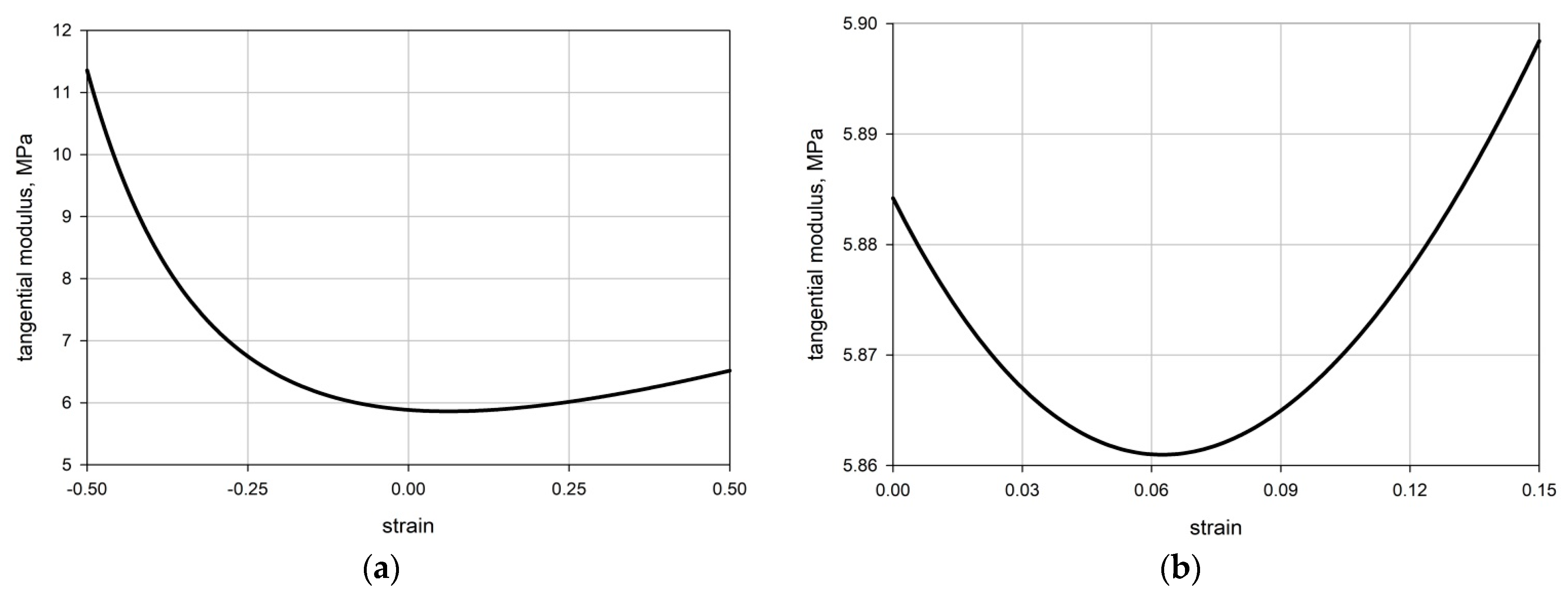
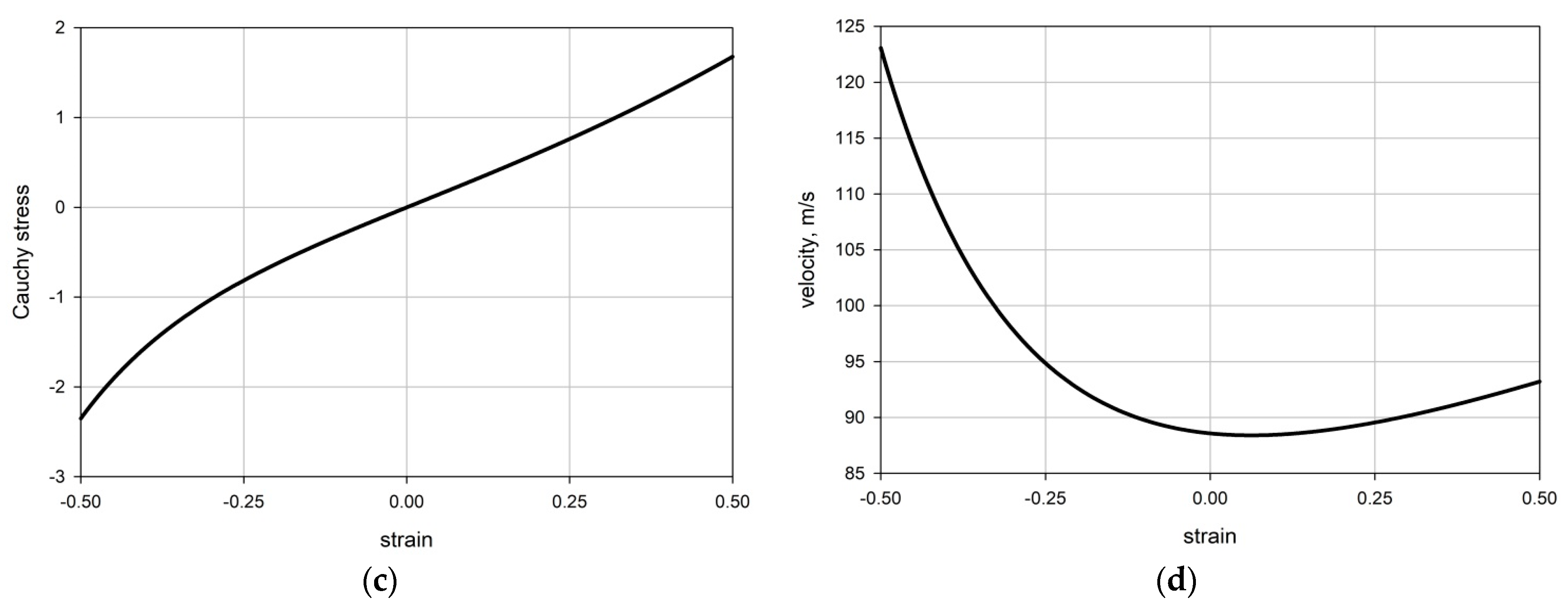
3.2.1. Physical Parameters

Herein, the medium-hard rubber [43] is modeled by the Mooney–Rivlin incompressible hyperelastic potential with the following physical parameters

$$C_{01}=0.0647 \mathrm{MPa}; C_{10}=0.916 \mathrm{MPa}; \rho =750 {\mathrm{kg}/\mathrm{m}}^3.$$

(33)

According to [43], these parameters refer to the 60-IRHD medium-hard rubber which is widely used in earthquake engineering [44] and in aviation and automotive tire manufacturing.

In account of Equation (33) and Expressions (16) and (17) for Cauchy stress and tangential modulus, respectively, these allow us to construct the following plots; see Figure 2a–c.

Analyzing the plot in Figure 2 reveals that (i) the tangential modulus is not monotonic in the range $\epsilon \in \left[-0.5,0.5\right]$; (ii) the minimum is attained at $\epsilon \approx 0.062$; and (iii) the stress–strain variation is monotonic in the studied range $\epsilon \in \left[-0.5,0.5\right]$.

3.2.2. Waves at Harmonic Excitation

Fairly large harmonic loadings with frequencies varied in a range $\omega \in \left[1,30\right]$ rad/s. The loading amplitude σ₀ = 1 was chosen to ensure the strain amplitude near the left end was ${\epsilon }_0\approx 0.3$. The plot in Figure 2d shows that slower moving parts of the wave at a smaller $\epsilon$ will be overtaken by the faster moving parts, especially those related to large negative strains; according to [24], these effects will eventually lead to the appearance of shock wave fronts. The relative displacements, distances, time, and specific energies appearing in Figure 3 are, respectively, defined as

$$U*=\frac{U}{\omega c_0}; l*=\frac{l}{\omega c_0}; t*=\frac{\omega t}{2\pi } E*=\frac{E}{\rho c_0^2},$$

(34)

where c₀ is the limiting wave velocity defined by Equation (19) and the relative displacement magnitude is defined as max (U*) over time.

The performed numerical analysis reveals (i) considerable attenuation of the wave amplitudes with distance from the excitation source, Figure 3a; (ii) a decrease in both specific strain and specific kinetic energy with distance in expense of the rise in specific thermal energy, Figure 3b; and (iii) the appearance of multiple shock wave fronts corresponding to the multiple overtaking occurring when faster moving pulses with negative strain overtake slower moving pulses with positive strain, see Figure 3c. Moreover, the propagating multiple shock wave fronts seen in Figure 3c indicate that all material is involved in the process of the mechanical energy dissipation and the increase in entropy and heat release; thus, in a purely mechanical system obeying the Mooney–Rivlin equation of state, the initially harmonic excitation leads to the attenuation of acoustic waves.

Another remark concerns the appearance of shock wave fronts in a rod modelled by a neo-Hookean potential, which follows (13) by taking $C_{01}=0$ [15]. This yields:

$$W=C_{10}\left({\lambda }^2+\frac{2}{\lambda }-3\right)=C_{10}\left({(1+\epsilon )}^2+\frac{2}{(1+\epsilon )}-3\right)$$

(35)

and

$$E(\epsilon )\equiv {\mathsf{\partial }}_{\epsilon }\sigma =2C_{10}\frac{3+9\epsilon +12{\epsilon }^2+8{\epsilon }^3+2{\epsilon }^4}{{\left(1+\epsilon \right)}^3},$$

(36)

from where the speed of sound becomes:

$$c(\epsilon )=\sqrt{\frac{2C_{10}}{\rho }}\sqrt{\frac{3+9\epsilon +12{\epsilon }^2+8{\epsilon }^3+2{\epsilon }^4}{{\left(1+\epsilon \right)}^3}}$$

(37)

Now, taking $C_{10}=0.916 \mathrm{MPa}$, as in Equation (33), we can observe shock wave fronts and the associated dissipation of mechanical energy in a rod modelled by the neo-Hookean potential. It is interesting to note that plots for the spatial variation in specific strain, kinetic and thermal energy, along with the displacement field for neo-Hookean potential, are almost identical to the plots shown in Figure 3 for the Mooney–Rivlin potential. This is explained by a small material constant $C_{01}$ in Equation (33), which, for the neo-Hookean potential, produces visually indistinguishable results. And finally, no dissipation of mechanical energy and shock wave fronts were observed in a linear elastic medium [24,34].

4. Concluding Remarks

The analysis of the harmonic excitation applied to the edge of a one-dimensional semi-infinite rod obeying the Mooney–Rivlin hyperelastic equation of state, which corresponds to a medium-hard rubber material [43,44], revealing:

(i)

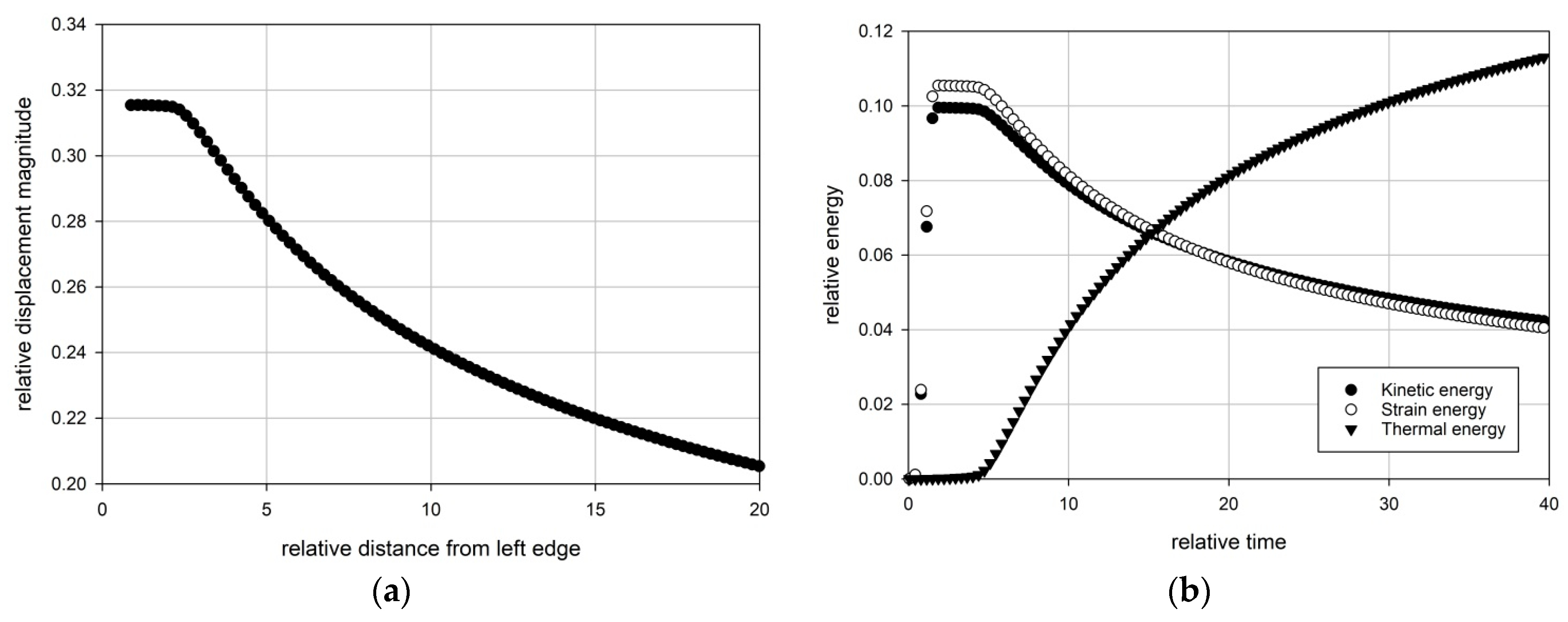
the initially harmonic wave attenuates with the distance, see Figure 3a;

(ii)

both strain and kinetic energy decrease with the distance from the excitation source, along with the simultaneous increase in the thermal energy, see Figure 3b;

(iii)

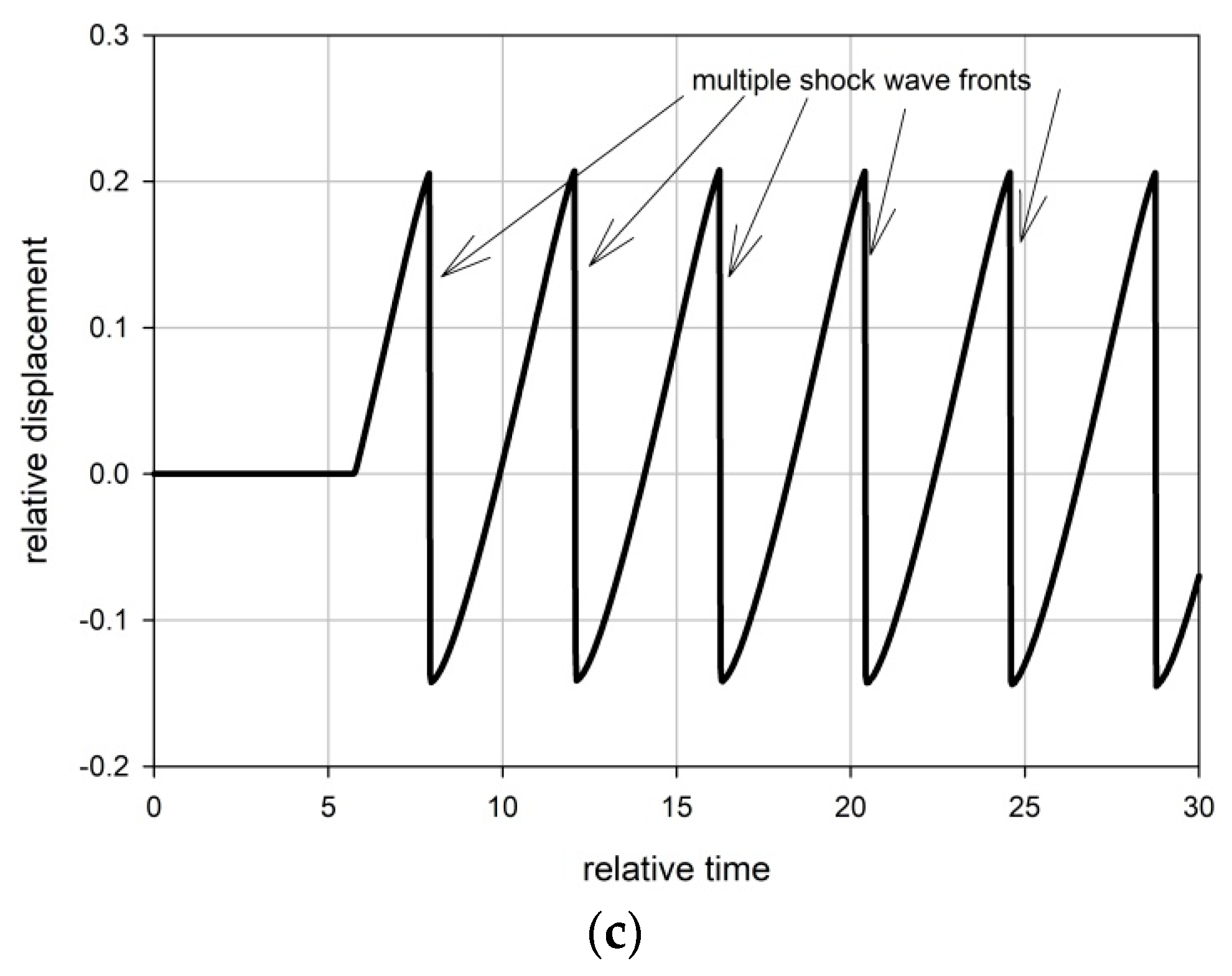
the appearance of the multiple shock wave fronts between positive and negative strain pulses, see Figure 3c.

These phenomena, observed apparently for the first time for a material with continuous (and smooth) nonlinearity, are caused by the formation and propagation of shock wave fronts, as was theoretically predicted more than 60 years ago [24]. It should also be noted that in materials with a discontinuous nonlinearity, as in the case of bi-modular materials, the appearance of shock wave fronts in solid media was previously detected, see [22,23].

It should also be emphasized that the discussed phenomena can be used in creating a new type of non-reflecting boundary elements without viscous dissipation [45], compared with more traditional elastic-viscous elements [46,47] used for non-reflecting boundaries. Another area for possible application resides in the development of seismic barriers [48,49] used for protection from Rayleigh and Rayleigh–Lamb seismic waves, along with various applications in vibration protection [50,51,52,53,54,55,56]. Actually, the analyzed non-linear elastic media modeled by the Mooney–Rivlin equation of state and exhibiting the mechanical energy dissipation at the acoustic wave propagation open up a new approach in creating seismic and vibration isolation devices.

Another remark concerns the observed heat production at the propagation of the (initially) harmonic waves in a purely mechanical nonlinear elastic system without viscosity and plastic dissipation. Accounting for the mechanical energy dissipation and simultaneous heat release at the propagation of harmonic waves is of crucial importance for a better understanding of the operation of seismic and vibration isolators utilizing nonlinear materials obeying the Mooney–Rivlin equation of state. Actually, the use of these materials in seismic and vibration protection devices opens up a new perspective for reducing mechanical energy in a purely mechanical system without viscous or dry friction elements, which can be especially important in seismic protection from the high intensity various surface acoustic waves (SAW) arising in the epicentral regions [57,58,59].

And finally, it can be anticipated that the observed phenomena can take place in other types of non-linear elastic materials with a smooth dependence of physical properties on strain, e.g., modelled by the Arruda–Boyce, Ogden, and Yeoh potentials. It should also be noted from the previous works on harmonic and shock waves in bi-modular materials with an abrupt change in material properties at vanishing strain [16,20,23] that it was implicitly assumed that the discontinuity in material properties is the key factor in the appearance of the shock wave fronts. However, the current research clearly demonstrates that shock wave fronts, causing dissipation of mechanical energy, appear in media with continuous and even smooth dependences of material properties on strain. As was noted above, the appearance and propagation of shock wave fronts in the considered media can be used in a new type of vibration and seismic isolating devices, which ensure vibration reduction from different types of bulk and surface waves, including those that arise in the epicentral zones of earthquakes [60,61,62,63,64].

References

1. Rankine, W.J.M. On the thermodynamic theory of waves of finite longitudinal disturbances. Phil. Trans. R. Soc. Lond. 1870, 160, 277–286. [Google Scholar]
2. Cui, W.; Mu, X.; Chen, W.; Stephens, T.A.; Bledsoe, B.P. Emergency control scheme for upstream pools of long-distance canals. Irrig. Drain 2018, 68, 218–226. [Google Scholar] [CrossRef]
3. Hunter, J.K.; Keller, J.B. Caustics of nonlinear waves. Wave Motion 1987, 9, 429–443. [Google Scholar] [CrossRef]
4. Sasoh, A.; Ohtani, T.; Mori, K. Pressure effect in a shock-wave plasma interaction induced by a focused laser pulse. Phys. Rev. Lett. 2006, 97, 205004. [Google Scholar] [CrossRef] [PubMed]
5. Znamenskaya, I.A.; Koroteev, D.A.; Lutsky, A.E. Discontinuity breakdown on shock wave interaction with nanosecond discharge. Phys. Fluids 2008, 20, 056101. [Google Scholar] [CrossRef]
6. Kulikovskii, A.G. Multi-parameter fronts of strong discontinuities in continuum mechanics. J. Appl. Math. Mech. 2011, 75, 378–389. [Google Scholar] [CrossRef]
7. Zhang, S. Shock wave evolution and discontinuity propagation for relativistic superfluid hydrodynamics with spontaneous symmetry breaking. Phys. Lett. B 2014, 729, 136–142. [Google Scholar] [CrossRef]
8. Morduchow, M.; Libby, P.A. On the distribution of entropy through a shock wave. J. Mécanique 1965, 4, 191–213. [Google Scholar]
9. Zeldovich, Y.B.; Raizer, Y.P. Physics of Shock Waves and High-Temperature Hydrodynamic Phenomena, 2nd ed.; Academic Press: New York, NY, USA, 1967. [Google Scholar]
10. Ridah, S. Shock waves in water. J. Appl. Phys. 1988, 64, 152–158. [Google Scholar] [CrossRef]
11. Arima, T.; Taniguchi, S.; Ruggeri, T.; Sugiyama, T. Extended thermodynamics of dense gases. Contin. Mech. Thermodyn. 2012, 24, 271–292. [Google Scholar] [CrossRef]
12. Velasco, R.M.; Garcia-Colin, L.S.; Uribe, F.J. Entropy production: Its role in nonequilibrium thermodynamics. Entropy 2011, 13, 82–116. [Google Scholar] [CrossRef]
13. Margolin, L.G. Nonequilibrium entropy in a shock. Entropy 2017, 19, 368. [Google Scholar] [CrossRef]
14. Hafskjold, B.; Bedeaux, D.; Kjelstrup, S.; Wilhelmsen, A. Nonequilibrium thermodynamics of surfaces captures the energy conversions in a shock wave. Chem. Phys. Lett. X 2020, 7, 100054. [Google Scholar] [CrossRef]
15. Pence, T.J.; Gou, K. On compressible versions of the incompressible neo-Hookean material. Math. Mech. Solids 2015, 20, 157–182. [Google Scholar] [CrossRef]
16. Maslov, V.P.; Mosolov, P.P. General theory of the solutions of the equations of motion of an elastic medium of different moduli. J. Appl. Math. Mech. 1985, 49, 322–336. [Google Scholar] [CrossRef]
17. Ostrovsky, L.A. Wave processes in media with strong acoustic nonlinearity. J. Acoust. Soc. Am. 1991, 90, 3332–3337. [Google Scholar] [CrossRef]
18. Kuznetsov, S.V. Abnormal dispersion of flexural Lamb waves in functionally graded plates. Z. Angew. Math. Mech. 2019, 70, 89. [Google Scholar] [CrossRef]
19. Lucchesi, M.; Pagni, A. Longitudinal oscillations of bimodular rods. Int. J. Struct. Stab. Dyn. 2005, 5, 37–54. [Google Scholar] [CrossRef]
20. Gavrilov, S.N.; Herman, G.C. Wave propagation in a semi-infinite heteromodular elastic bar subjected to a harmonic loading. J. Sound Vib. 2012, 331, 4464–4480. [Google Scholar] [CrossRef]
21. Naeeni, M.R.; Eskandari-Ghadi, M.; Ardalan, A.A.; Pak, R.Y.S.; Rahimian, M.; Hayati, Y. Coupled thermoviscoelastodynamic Green’s functions for bi-material half-space. Z. Angew. Math. Mech. 2015, 95, 260–282. [Google Scholar] [CrossRef]
22. Li, S.J.; Brun, M.; Djeran-Maigre, I.; Kuznetsov, S. Hybrid asynchronous absorbing layers based on Kosloff damping for seismic wave propagation in unbounded domains. Comput. Geotech. 2019, 109, 69–81. [Google Scholar] [CrossRef]
23. Kuznetsova, M.; Khudyakov, M.; Sadovskii, V. Wave propagation in continuous bimodular media. Mech. Adv. Mater. Struct. 2021, 29, 3147–3162. [Google Scholar] [CrossRef]
24. Truesdell, C. General and exact theory of waves in finite elastic strain. Arch. Rat. Mech. Anal. 1961, 8, 263–296. [Google Scholar] [CrossRef]
25. Coleman, B.D.; Gurtin, M.E.; Herrera, I. Waves in materials with memory, I. The velocity of one-dimensional shock and acceleration waves. Arch. Rat. Mech. Anal. 1965, 19, 1–19. [Google Scholar] [CrossRef]
26. Truesdell, C. On curved shocks in steady plane flow of an ideal fluid. J. Aeronaut. Sci. 1952, 19, 826–834. [Google Scholar] [CrossRef]
27. Boulanger, P.; Hayes, M.A. Finite amplitude waves in Mooney–Rivlin and Hadamard materials. In Topics in Finite Elasticity; Hayes, M.A., Soccomandi, G., Eds.; Springer: Vienna, Austria, 2001. [Google Scholar]
28. Liu, C.; Cady, C.M.; Lovato, M.L.; Orler, E.B. Uniaxial tension of thin rubber liner sheets and hyperelastic model investigation. J. Mater. Sci. 2015, 50, 1401–1411. [Google Scholar] [CrossRef]
29. Goldstein, R.V.; Kuznetsov, S.V. Long-wave asymptotics of Lamb waves. Mech. Solids 2017, 52, 700–707. [Google Scholar] [CrossRef]
30. Hashiguchi, K. Nonlinear Continuum Mechanics for Finite Elasticity-Plasticity; Elsevier: New York, NY, USA, 2020. [Google Scholar]
31. LeVeque, R.J. Numerical Methods for Conservation Laws; Birkhäuser: Boston, MA, USA, 1992. [Google Scholar]
32. Press, W.H.; Teukolsky, S.A.; Vetterling, W.T.; Flannery, B.P. Numerical Recipes: The Art of Scientific Computing, 3rd ed.; Cambridge University Press: New York, NY, USA, 2007. [Google Scholar]
33. Djeran-Maigre, I.; Kuznetsov, S.V. Velocities, dispersion, and energy of SH-waves in anisotropic laminated plates. Acoust. Phys. 2014, 60, 200–207. [Google Scholar] [CrossRef]
34. Truesdell, C.; Noll, W. The Non-Linear Field Theories of Mechanics, 3rd ed.; Springer: Berlin/Heidelberg, Germany, 2004. [Google Scholar]
35. Kuznetsov, S.V. Closed form analytical solution for dispersion of Lamb waves in FG plates. Wave Motion 2019, 84, 1–7. [Google Scholar] [CrossRef]
36. Kuznetsov, S.V. Lamb waves in stratified and functionally graded plates: Discrepancy, similarity, and convergence. Waves Random Complex Media 2019, 31, 1540–1549. [Google Scholar] [CrossRef]
37. Ilyashenko, A.V.; Kuznetsov, S.V. Pochhammer–Chree waves: Polarization of the axially symmetric modes. Arch. Appl. Mech. 2018, 88, 1385–1394. [Google Scholar] [CrossRef]
38. Lion, A. On the large deformation behaviour of reinforced rubber at different temperatures. J. Mech. Phys. Solids 1997, 45, 1805–1834. [Google Scholar] [CrossRef]
39. Lax, P.D. Hyperbolic Systems of Conservation Laws and the Mathematical Theory of Shock Waves; SIAM: Philadelphia, PA, USA, 1972. [Google Scholar]
40. Belytschko, T.; Liu, W.K.; Moran, B.; Elkhodary, K. Nonlinear Finite Elements for Continua and Structures, 2nd ed.; Wiley: New York, NY, USA, 2013. [Google Scholar]
41. Dumbser, M. Arbitrary-Lagrangian–Eulerian ADER-WENO finite volume schemes with time-accurate local time stepping for hyperbolic conservation laws. Comput. Methods Appl. Mech. Eng. 2014, 280, 57–83. [Google Scholar] [CrossRef]
42. Neto, M.A.; Amaro, A.; Roseiro, L.; Cirne, J.; Leal, R. Finite Element Method for Trusses. In Engineering Computation of Structures: The Finite Element Method; Springer: Berlin/Heidelberg, Germany, 2015. [Google Scholar]
43. Jerrams, S.J.; Bowen, J. Modelling the behaviour of rubber-like materials to obtain correlation with rigidity modulus tests. WIT Trans. Model. Simul. 1995, 12, CMEM950561. [Google Scholar]
44. Chen, J.; Garcia, E.S.; Zimmerman, S.C. Intramolecularly cross-linked polymers: From structure to function with applications as artificial antibodies and artificial enzymes. Acc. Chem. Res. 2020, 53, 1244–1256. [Google Scholar] [CrossRef]
45. D’Amato, M.; Gigliotti, R.; Laguardia, R. Seismic isolation for protecting historical buildings: A case study. Front. Built Environ. 2019, 5, 87. [Google Scholar] [CrossRef]
46. Goldstein, R.V.; Dudchenko, A.V.; Kuznetsov, S.V. The modified Cam-Clay (MCC) model: Cyclic kinematic deviatoric loading. Arch. Appl. Mech. 2016, 86, 2021–2031. [Google Scholar] [CrossRef]
47. Carcione, J.M.; Kosloff, D. Representation of matched-layer kernels with viscoelastic mechanical models. Int. J. Numer. Anal. Model. 2013, 10, 221–232. [Google Scholar]
48. Li, S.; Brun, M.; Djeran-Maigre, I.; Kuznetsov, S. Benchmark for three-dimensional explicit asynchronous absorbing layers for ground wave propagation and wave barriers. Comput. Geotech. 2021, 131, 103808. [Google Scholar] [CrossRef]
49. Kuznetsov, S. Fundamental and singular solutions of Lame equations for media with arbitrary elastic anisotropy. Q. Appl. Math. 2005, 63, 455–467. [Google Scholar] [CrossRef]
50. Kuznetsov, S. Seismic waves and seismic barriers. Acoust. Phys. 2011, 57, 420–426. [Google Scholar] [CrossRef]
51. Haris, A.; Alevras, P.; Mohammadpour, M.; Mahony, M.O. Design and validation of a nonlinear vibration absorber to attenuate torsional oscillations of propulsion systems. Nonlinear Dyn. 2020, 100, 33–49. [Google Scholar] [CrossRef]
52. Safari, S.; Tarinejad, R. Parametric study of stochastic seismic responses of base-isolated liquid storage tanks under near-fault and far-fault ground motions. J. Vib. Control 2018, 24, 5747–5764. [Google Scholar] [CrossRef]
53. Carranza, J.C.; Brennan, M.J.; Tang, B. Sources and propagation of nonlinearity in a vibration isolator with geometrically nonlinear damping. J. Vibr. Acoust. 2015, 138, 024501. [Google Scholar] [CrossRef]
54. Zhu, Y.P.; Lang, Z.Q. Beneficial effects of antisymmetric nonlinear damping with application to energy harvesting and vibration isolation under general inputs. Nonlinear Dyn. 2022, 108, 2917–2933. [Google Scholar] [CrossRef]
55. Harris, C.; Piersol, A. Harris Shock and Vibration Handbook, 5th ed.; McGraw-Hill: New York, NY, USA, 2002. [Google Scholar]
56. Kuznetsov, S. Subsonic Lamb waves in anisotropic plates. Q. Appl. Math. 2002, 60, 577–587. [Google Scholar] [CrossRef]
57. Carboni, B.; Lacarbonara, W. Nonlinear dynamic characterization of a new hysteretic device: Experiments and computations. Nonlinear Dyn. 2016, 83, 23–39. [Google Scholar] [CrossRef]
58. Kuznetsov, S. Surface waves of non-Rayleigh type. Q. Appl. Math. 2003, 61, 575–582. [Google Scholar] [CrossRef]
59. Tian, J.H.; Luo, Y.; Zhao, L. Regional stress field in Yunnan revealed by the focal mechanisms of moderate and small earthquakes. Earth Planet. Phys. 2019, 3, 243–252. [Google Scholar] [CrossRef]
60. Ben-Menahem, S.; Singh, S.J. Seismic Waves and Sources; Springer: New York, NY, USA, 2011. [Google Scholar]
61. Sutton, G.H.; Mitronovas, W.; Pomeroy, P.W. Short-period seismic energy radiation patterns from underground nuclear explosions and small-magnitude earthquakes. Bull. Seismol. Soc. Am. 1967, 57, 249–267. [Google Scholar] [CrossRef]
62. Dudchenko, A.V.; Dias, D. Vertical wave barriers for vibration reduction. Arch. Appl. Mech. 2020, 91, 257–276. [Google Scholar] [CrossRef]
63. Placinta, A.-O.; Borleanu, F.; Moldovan, I.-A.; Coman, A. Correlation between seismic waves velocity changes and the occurrence of moderate earthquakes at the bending of the Eastern Carpathians (Vrancea). Acoustics 2022, 4, 934–947. [Google Scholar] [CrossRef]
64. Petrescu, L.; Borleanu, F.; Radulian, M.; Ismail-Zadeh, A.; Maţenco, L. Tectonic regimes and stress patterns in the Vrancea Seismic Zone: Insights into intermediate-depth earthquake nests in locked collisional settings. Tectonophysics 2021, 799, 228688. [Google Scholar] [CrossRef]
Figure 1. Semi-infinite rod with harmonic force loading applied at the left end.
Applsci 13 10037 g001
Figure 2. (a) Tangential modulus; (b) tangential modulus in the vicinity of extremum; (c) Cauchy stress; (d) speed of propagation.
Applsci 13 10037 g002aApplsci 13 10037 g002b
Figure 3. Mooney–Rivlin potential: (a) attenuation of the relative displacement magnitude; (b) attenuation of specific strain and kinetic energy and an increase in thermal energy; (c) appearing multiple shock wave fronts at overtaking pulses of different signs at a point located at a relative distance of 100 from the left edge.
Applsci 13 10037 g003aApplsci 13 10037 g003b
Disclaimer/Publisher’s Note: The statements, opinions and data contained in all publications are solely those of the individual author(s) and contributor(s) and not of MDPI and/or the editor(s). MDPI and/or the editor(s) disclaim responsibility for any injury to people or property resulting from any ideas, methods, instructions or products referred to in the content.