An Improved Visual SLAM Method with Adaptive Feature Extraction

Abstract

The feature point method is the mainstream method to accomplish inter-frame estimation in visual Simultaneous Localization and Mapping (SLAM) methods, among which the Oriented FAST and Rotated BRIEF (ORB) feature-based method provides an equilibrium of accuracy as well as efficiency. However, the ORB algorithm is prone to clustering phenomena, and its unequal distribution of extracted feature points is not conducive to the subsequent camera tracking. To solve the above problems, this paper suggests an adaptive feature extraction algorithm that first constructs multiple-scale images using an adaptive Gaussian pyramid algorithm, calculates adaptive thresholds, and uses an adaptive meshing method for regional feature point detection to adapt to different scenes. The method uses Adaptive and Generic Accelerated Segment Test (AGAST) to speed up feature detection and the non-maximum suppression method to filter feature points. The feature points are then divided equally by a quadtree technique, and the orientation of those points is determined by an intensity centroid approach. Experiments were conducted on publicly available datasets, and the outcomes demonstrate the algorithm has good adaptivity and solves the problem of a large number of corner point clusters that may result from using manually set detection thresholds. The RMSE of the absolute trajectory error of SLAM applying this method on four sequences of TUM RGB-D datasets is decreased by 13.88% when compared with ORB-SLAM3. It is demonstrated that the algorithm provides high-quality feature points for subsequent image alignment, and the application to SLAM improves the reliability and accuracy of SLAM.

1. Introduction

SLAM refers to the model in which a subject equipped with some sensors creates a map of the surroundings during its motion and estimates its own velocity without any a priori information about the environment [1]. SLAM technology is widely used in the fields of autonomous driving, drones, and robot navigation. It can help devices determine their own position and the terrain and obstacles of the surrounding environment. Or, combined with a variety of information, such as semantic information, and perceptual systems, such as target recognition [2], instance segmentation [3], etc., more complex tasks can also be accomplished by SLAM technology.

SLAM is mainly divided into laser SLAM and visual SLAM because of the different sensors it carries. In terms of theory and engineering, laser SLAM is more mature, and it has practical applications in industrial industries. The SLAM system called Visual SLAM (VSLAM) relies heavily on pictures to provide environment-aware data. Visual SLAM, which primarily focuses on calculating camera poses and constructing 3D maps using the multi-view geometry approach, is still in the laboratory research stage and has fewer practical applications. However, compared to laser sensors that can only provide single spatial structure perception information, visual sensors have great advantages and the potential to improve inter-frame estimation accuracy and loop closing detection accuracy with their abundant sense information, which includes texture and color [4]. Moreover, cameras are inexpensive and can provide rich environmental information, so VSLAM solutions where a camera serves as the primary sensor are extremely intriguing.

The processing of SLAM systems is frequently divided into two phases: front-end inter-frame estimation and back-end optimization. In order to accomplish feature point tracking and mapping in parallel, PTAM [5], which distinguishes between the front-end and back-end, was the first to propose and implement this processing. Front-end interframe estimation is based on the sensor information between two adjacent frames to obtain an estimate of the motion during that time interval, also known as visual odometry.

There are two categories of inter-frame estimation implementation techniques in the front-end: direct methods and feature point methods.

The direct method makes direct use of image information, which relies on dense pixel points to estimate structure and motion directly by minimizing an error measure that is based on the image’s pixel-level intensities [6]. However, because the approach is dependent on the assumption of grayscale invariance, it cannot be applied to scenes with significant illumination changes and can lead to tracking failure if the movement of the camera is too large.

The feature point method extracts a collection of salient image characteristics (such as corner points) from every image, matches them in consecutive frames using invariant feature descriptors of this set, and then uses the epipolar geometry to steadily recover camera motion and structure. In back-end optimization, camera poses and maps are optimized by minimizing feature point reprojection errors. In loop closing detection, feature correspondence with old landmarks is established by feature descriptors, which increases both the constraints in BA (Bundle Adjustment) optimization, which improves the accuracy of the optimized trajectory, and the relocalization capability, resulting in a more robust system. Feature point methods rely on effective feature detectors and descriptors that enable matching images with large variations in illumination and viewpoint.

The feature point method calculates camera motion via a part of the image’s points. Although the feature point method takes significant amounts of computational resources in the process of calculating descriptors, it has the excellent feature of being insensitive to changes in illumination and dynamic environmental changes. It can also be understood that the feature point method has no rigid requirements for environmental conditions; therefore, it is highly adaptable, so it holds a mainstream position in visual odometry.

In SLAM, back-end optimization is not performed in real time. To obtain highprecision pose estimation, the local or global drift error is eliminated by only activating it when a frame is chosen as a key frame. Therefore, the feature extraction speed has a significant impact on the SLAM’s real-time performance.

Additionally, the majority of feature extraction thresholds used in existing SLAM feature detection are set manually. This could result in a lot of corner clusters and the generation of too many feature points, which would not be able to meet the requirements of various images for feature point extraction and increase the complexity of subsequent image alignment.

Furthermore, the robustness of SLAM is more strongly influenced by the robustness, orientation invariance, and scale invariance of extracted feature points. However, the majority of feature extraction techniques use an image pyramid to give the features scale invariance while simultaneously increasing computation. Many features that are faster to extract mostly lack scale invariance. How to balance them is also an important issue.

This work proposes an adaptive feature extraction approach to address the above issues while also increasing the real-time speed and robustness of SLAM. The following is a summary of this paper’s main contributions:

• This paper designs the detection thresholds for AGAST based on the image’s overall grayscale information, which can be adjusted to varied situations and extract an appropriate amount of feature points with high quality.
• Image pyramids are adaptively built for images of various sizes, and feature detection is accomplished by utilizing the adaptive meshing method and AGAST algorithm. This could adapt to various inputs and decrease unnecessary calculations.
• Following the detection of feature points, we utilize the Non-Maximum Suppression (NMS) method to filter the feature points and combine the quadtree algorithm to homogenize them, which can avoid corner point clustering. We calculate the feature point orientation using the intensity centroid method to provide orientation invariance for it, which is conducive to subsequent feature matching.

2. Related Work

2.1. Visual SLAM

Currently, there are many excellent and mature solutions for SLAM tasks based on the direct method. The DTAM system was presented by R. Newcombe et al. in 2011 [7]. Instead of using feature extraction, this system relies on dense pixel points for real-time tracking and map building, comparing the input image with the synthetic view, and then calculating the difference between the image and the view to accomplish localization tracking. However, since this system is a monocular system, it needs to calculate the depth information of each pixel point, so it is computationally expensive. In 2014, ref. [8] suggested LSD-SLAM. This system randomly sets the initial depth value for each pixel point, reconstructs the map for regions with significant gradient changes, and also uses the synthetic view generated by the map to optimize the estimated camera motion. However, it is tough to accurately calculate the depth information of the whole image because it is not possible to estimate regions without texture. In 2017, Wang Rui et al. proposed a completely straightforward system called DSO [9]. This system divides each picture into blocks and selects high-intensity feature points as candidates for reconstructing the map. Simultaneously, it uses geometric and photometric cameras to eliminate the error factor and calibrate the results to decrease the cumulative error. Tested on a publicly available dataset, the system achieves high localization accuracy and is one of the better algorithms in the current direct method.

While the feature point method was initially used in VSLAM systems in 2007, the literature [1] presented the MonoSLAM system as the first monocular VSLAM system that could run in real-time. To track extremely sparse feature points at the front-end, the system employs an extended Kalman filter as the back-end. In 2009, ref. [5] suggested the monocular SLAM system PTAM. This system was the first to parallelize the tracking and map-building processes. PTAM was the first system to use nonlinear optimization at the back-end instead of traditional filters, and it proposed the keyframes mechanism so that it does not have to process each image finely but instead processes a smaller number of key images to optimize its trajectory and map. Following PTAM, VSLAM research increasingly shifted to the back-end, which became dominated by nonlinear optimization.

The monocular ORB-SLAM system put forward by [10] represented a peak of mainstream feature point SLAM in 2015. A year later, the authors [11] proposed the ORB-SLAM2 system to address the drawback that ORB-SLAM can only use monocular sensors. ORB-SLAM2 was the first complete the open-source SLAM scheme for monocular, stereo, and RGB-D cameras. And since then, many excellent visual SLAM systems have been improved and optimized as a foundation for ORB-SLAM2.

Research in [12] proposed the feature-based, tightly coupled VIO system ORB-SLAM3, which builds on ORB-SLAM2 to also conduct visual, visual inertial, and multi-map SLAM utilizing pinhole and fisheye lens models. OV²SLAM [13] is a fully online and versatile real-time visual SLAM system suggested in 2021 by Maxime Ferrera and collaborators. The system restricts the extraction of features to keyframes and tracks them in the following frames using minimized photometric errors, significantly reducing the computing effort. And it integrates an online BoW method that creates its vocabulary tree step-by-step using feature descriptors computed from keyframes, which can help it adapt to the environment better. The system achieves better accuracy and real-time performance.

2.2. Image Feature Point

The concept of image feature points was suggested by Moravec firstly [14]. After that, related scholars at home and abroad studied this problem one after another. Lowe et al. [15] proposed the Scale-Invariant Feature Transformation (SIFT) algorithm, which extracts feature points with better scale invariance and rotation invariance. Additionally, it may give reliable matching for a variety of affine distortions, 3D perspective changes, noise increases, and illumination changes. However, it has high operational complexity and takes a long time to extract features. In response to the question, ref. [16] suggested Speeded-Up Robust Feature (SURF). This SURF algorithm improves the SIFT algorithm using integral maps, approximate Hessian matrices, and Haar wavelet transformation operations, and although it improves the algorithm’s performance, it still takes longer to calculate the feature descriptors and fails to satisfy the SLAM real-time requirements.

In 2010, Rosten et al. proposed the Feature from Accelerated Segment Test (FAST) algorithm [17], which is fast and can quickly detect corner points in images, but it does not produce multiscale features, has no orientation information, and does not have rotational invariance. In 2011, Rublee et al. presented the ORB algorithm [18], which detects feature points using the FAST technique and obtains the feature descriptors of the image by calculating Binary Robust Independent Elementary Features (BRIEF) algorithm, which is more robust to noise. Therefore, the ORB algorithm extracts features more quickly. Under the same conditions, the extraction speed of feature points is faster than SURF and SIFT algorithms, which can fulfill the system’s real-time needs, but its robustness is not as good as SIFT, and there is no scale invariance. Therefore, the algorithm is prone to feature point redundancy, and these redundant feature points will lead to mismatches in image matching. The ORB-SLAM is calculated around the ORB feature, which is an excellent compromise between efficiency and accuracy at this stage of computing platforms. And the ORB feature provides descriptors that enable loop closing detection and relocation during a large range of motion. In response to the problems existing in the feature extraction algorithm, many scholars have improved it. Research in [19] improved the original ORB and suggested a better ORB algorithm based on region division, which ensures an improved uniformity of extracted feature points; however, feature point mismatch still exists. Mair et al. proposed the AGAST algorithm [20], which is an adaptive multi-scale fast corner point extraction algorithm and is an improved version of the FAST algorithm. The technique increases feature extraction speed while also having strong scale invariance. Aiming at the impact of illumination changes on feature tracking, ref. [21] used the AKAZE detector to extract feature points after they constructed a color space with constant illumination based on adaptive histogram equalization and dark channel prior theory. This technique increases the accuracy of extracting and matching image feature points in the event of significant changes in illumination. Research in [22] enhanced the feature method of point-line combination and implemented a local adaptive threshold calculation method and a new meshing technique in ORB feature extraction. After meshing, the threshold is calculated separately for each image block, which improves the adaptive ability of feature extraction.

Deep learning has advanced quickly in the field of computer vision in recent years. Many scholars have applied deep learning to feature extraction tasks and achieved good results. In 2018, DeTone, D. et al. [23] proposed SuperPoint by using deep learning methods for feature extraction. It uses a single network and self-supervised methods to extract keypoints, but its network structure is large and time-consuming. To tackle this issue, Li, G.Q., et al. [24] designed a simpler convolutional neural network to detect keypoints and calculate descriptors, which reduced the time-consuming process of feature extraction. It can run on the graphics processor (GPU) in real time to meet the needs of SLAM’s real-time performance, but when it is applied to ORB-SLAM2, its time consumption can reach 5.2 times that of the original system. Zhao, X. et al. [25] designed a lightweight network for feature point detection and descriptor extraction that can run images with a size of 640 × 480 at a speed of 95 frames per second on a commercial GPU. We applied it to ORB-SLAM2 and tested it in the experimental environment of this paper. The speed is faster than the above methods, but when considered comprehensively, its performance in SLAM tasks is still not as good as ORB feature points.

We also enhance the ORB approach in this paper. We suggest a global adaptive threshold calculation method that computes the threshold for various images based on their gray information. We adaptively construct an image pyramid to provide scale invariance. Different from the predefined threshold in ORB-SLAM2 and the FAST threshold calculated for each image block after meshing the image pyramid in [22], we use the gray information of the entire image to calculate a global adaptive threshold, which reduces the amount of calculation before feature detection and takes into account the adaptability of the threshold. Additionally, we design an adaptive meshing technique to segment the pyramid image, allowing for the use of various detection thresholds in the same image. Different from ORB [18] using the FAST algorithm, we use the AGAST approach to detect feature points, which has better adaptability and extraction speed [20]. We apply the NMS method for filtering the detected feature points and eliminating the local dense feature points. The quad-tree algorithm is then applied to achieve equal division of feature points, similar to the feature extraction part of ORB-SLAM2. Then the direction of the feature points is calculated like the ORB algorithm.

3. Our Method

3.1. Improved Feature Extraction Algorithm

The framework of the enhanced feature extraction algorithm suggested in this article is shown in Figure 1, where the blue part is the pre-processing part before feature detection, the gray part is the feature detection part, and the orange part is the feature point assignment part. We will elaborate on the steps of this method in the following sections. After extracting features, the Rotated BRIEF algorithm is used to describe the features.

3.1.1. Calculate Global Adaptive Threshold

The setting of the feature extraction threshold has a significant impact on the number and quality of extracted feature points. Because the extraction of feature points depends on the image’s gray information, it is necessary to determine during feature detection whether and how many times the gray difference between a pixel and its surrounding pixels exceeds the threshold. The threshold represents the strictness of extracting feature points and reflects the gray difference between a pixel and its surrounding pixels. Therefore, based on the overall image’s gray information, we can determine whether the image’s gray change is obvious, similar to the contrast. The gray difference between the pixels and the surrounding pixels may be significant for images with obvious changes. At this time, selecting a smaller threshold will extract too many feature points, which will affect the speed of feature extraction, and those feature points that are extracted near the threshold have a low degree of recognition, which will affect the matching of subsequent feature points. If a larger threshold is selected, it may lead to the fact that the majority of pixels cannot meet the threshold and the extracted feature points are too few, which is not conducive to subsequent processing.

For adaptation to different scenarios, this work proposes an adaptive threshold calculation approach that can extract a sufficient number of feature points while simultaneously guaranteeing the quality of the feature points for better tracking. Different from ORB-SLAM2 [11], which sets a specific threshold value for feature extraction, this paper sets the threshold value for feature extraction by considering the image grayscale information. The thresholds are specifically derived from the following:

$$Threshold=({\displaystyle \frac{1}{n}}\sum _{x=1}^{width}\sum _{y=1}^{height}{(I(x,y)-\overline{I(x,y)})}^2)/\overline{I(x,y)},$$

(1)

$$\overline{I(x,y)}={\displaystyle \frac{1}{n}}\sum _{x=1}^{width}\sum _{y=1}^{height}I(x,y),$$

(2)

where n is the number of image pixels, $I(x,y)$ is each pixel’s gray value, and $\overline{I(x,y)}$ is the average gray value of the image. ${\displaystyle \frac{1}{n}}{\sum }_{x=1}^{width}{\sum }_{y=1}^{height}{(I(x,y)-\overline{I(x,y)})}^2$ is the variance of the image gray value.

3.1.2. Construct a Gaussian Pyramid

The previous approaches frequently employed the image pyramid with a fixed number of levels of 8 to offer scale invariance for features, such as ORB-SLAM3 [12,22]. The high layer of the image, which is scaled down to create the image pyramid, contains less image information when the image is small. In this case, the high-level image has little effect on scale invariance. The amount of calculation may increase when the pyramid’s layers are added. For the purpose of reducing the quantity of calculations and better tracking, this paper designs an adaptive image pyramid layer decision method, facing the input pictures with different resolutions. The number of layers is set as follows:

$$Level=\mathrm{Round}\left(\right(width+height)/200),$$

(3)

We divided the sum of the picture’s width and height by 200 and rounded up to obtain the number of levels of the pyramid’s construction plan because the picture’s proportions could not be taken into consideration when utilizing the picture’s area. After calculating the necessary number of pyramid layers, the picture is down-sampled based on the scale factor to generate an image of all pyramid layers and set the number of feature points to be acquired for each layer.

3.1.3. Adaptive Meshing of the Image Pyramid

To extract feature points using various thresholds within the same image, the image is divided into meshes. Feature points are extracted using lower thresholds on grids with less texture. It lessens the possibility that the feature points are only distributed in certain areas when compared to the extraction of feature points for the entire image. ORB-SLAM2 [11] uses the meshing method. However, it divides the image into multiple 30 × 30 grids during feature extraction for each layer of the image. Due to the different scenes and sizes of each image, using a single engineering empirical value of 30 to divide the grid causes the algorithm to be unable to adapt well to the external environment. In this study, we apply an adaptive algorithm to handle the grid division, and we divide each layer of the photo according to its area and the number of feature points it needs to extract. The side lengths of the grid are calculated as follows:

$$W_i=\alpha \sqrt{(widt{h}_i\times heigh{t}_i/N_i)},$$

(4)

where $W_i$ is the side length of the i-th layer image partition grid. $widt{h}_i$ and $heigh{t}_i$ are the picture’s width and height in layer i, respectively, and $N_i$ is the amount of feature points to be extracted from the picture in layer i. $\alpha$ is the scale factor.

After obtaining $W_i$, we can calculate the number of columns and rows per layer of the image, as shown below:

$$\left\{\begin{array}{c}Cols=\lfloor widt{h}_i/W_i\rfloor \hfill \\ Rows=\lfloor heigh{t}_i/W_i\rfloor \hfill \end{array}\right.$$

(5)

The next step is to traverse the number of rows and columns to extract the picture block’s features.

3.1.4. AGAST Extract Feature Points

We extract feature points using the AGAST method [20] from the divided grid image. The AGAST algorithm has added two states “not brighter” and “not darker” to the configuration space of FAST. The specific state is defined as follows:

$$S_{n\to x}=\left\{\begin{array}{cc}d,I_{n\to x}<I_n-t\hfill & \left(darker\right)\hfill \\ \overline{d},I_{n\to x}\ge I_n-t\wedge S_{n\to x}^{{}^{\prime }}=u\hfill & \left(notdarker\right)\hfill \\ s,I_{n\to x}\ge I_n-t\wedge S_{n\to x}^{{}^{\prime }}=\overline{b}\hfill & \left(similar\right)\hfill \\ s,I_{n\to x}\le I_n-t\wedge S_{n\to x}^{{}^{\prime }}=\overline{d}\hfill & \left(similar\right)\hfill \\ \overline{b},I_{n\to x}\le I_n-t\wedge S_{n\to x}^{{}^{\prime }}=u\hfill & \left(notbrighter\right)\hfill \\ b,I_{n\to x}>I_n+t\hfill & \left(brighter\right)\hfill \end{array}\right.,$$

(6)

where the state of a pixel for kernel n is denoted as $S_{n\to x}$, $S_{n\to x}^{{}^{\prime }}$ denotes the previous state, I represents the pixel luminance, and u indicates the unknown state. t represents the detection threshold; d indicates that the grayscale of the current point is darker than the center point; $\overline{d}$ indicates that the current point’s grayscale is non-darker than the center points’; s indicates that the grayscale of the current point is similar to the center point; b indicates that the current point’s grayscale is brighter than the center points’; $\overline{b}$ indicates that the grayscale of the current point is non-brighter than the center points’.

The AGAST [20] algorithm improves the Accelerated Segment Test (AST) module at the bottom of FAST. It uses an algorithm similar to reverse induction in the extended configuration space to find an optimal decision tree and combines the decision trees so that corner point detection can automatically adapt to changes in the external environment without having to reacquire the decision tree. AGAST improves the trinomial decision tree in the FAST algorithm into a binary tree, as shown in Figure 2. Once the pixel neighborhood changes, AGAST switches between two (or more) trees. In homogenous pixel neighborhoods, the left tree achieves fewer pixel evaluations (shorter decision paths), while the right tree is optimized for texture regions. AGAST dynamically and efficiently assigns decision trees based on the currently processed image information, improving the detection speed of the algorithm.

In order to ensure that enough feature points are extracted in areas with less texture, the global adaptive threshold obtained in a is first used as the initial value to detect feature points from the picture. The threshold is set to 1/4 of the original value, and feature points continue to be extracted when the obtained image feature points are insufficient.

3.1.5. NMS to Filter Feature Points

We refer to the concept of NMS of [26] to filter feature points and eliminate local dense feature points for the extracted feature points. The fundamental idea behind this method is to leave the most significant feature points in the region by the size of their corresponding values and suppress the insignificant feature points to increase the feature points’ accuracy and stability.

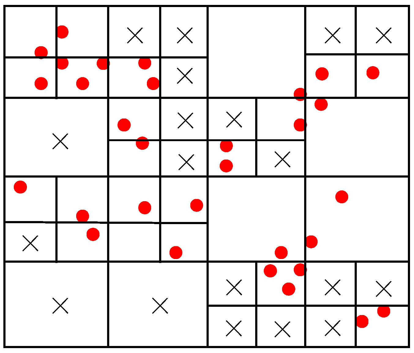
3.1.6. Divide Feature Points with Quad-Tree

Similar to [10], we additionally partition the feature points using the quad-tree approach to ensure that they are distributed equally. We initialize the nodes of each layer of the pyramid image, divide the image into four regions, and obtain four sub-nodes. We count how many feature points are present in each node. If a node does not include any feature points, it should be deleted; if it has just one, it ought to be marked as a leaf node, saved, and no longer split; if the node contains multiple feature points, it is called the parent node and continues to be divided. If all the current nodes are non-repartitionable or the sum of the number of leaf nodes and the number of parent nodes that need to continue to be partitioned reaches the requirement of the number of feature points, the partition is terminated. We retain the feature points in each node area with the largest response value. The division outcome for a target of 20 feature points is depicted in Figure 3, where the red dot is the feature point and the area of the fork is the deleted node area.

3.1.7. Intensity Centroid Method to Calculate the Orientation of Feature Points

According to the method proposed by [27], we define the direction of the feature point as the angle between the line connecting the feature point to the centroid of the picture block centering on the feature point and the horizontal direction. Shown in Figure 4a is an example of an image block. The centroid calculation formula for the image block is as follows:

$$Q=({\displaystyle \frac{m_{10}}{m_{00}}},{\displaystyle \frac{m_{01}}{m_{00}}}),$$

(7)

where m stands for the moment of the region, which is calculated as follows:

$$\begin{array}{c}\hfill m_{10}=\sum _{x,y}xI(x,y),\\ \hfill m_{01}=\sum _{x,y}yI(x,y),\\ \hfill m_{00}=\sum _{x,y}I(x,y).\end{array}$$

(8)

This allows us to determine the feature points’ orientation as follows:

$$\theta =arctan\left({\displaystyle \frac{m_{01}}{m_{10}}}\right)$$

(9)

The orientation of the feature points provides rotational invariance for the feature points. It is illustrated in Figure 4c as the image of Figure 4b after rotation, and the orientation of the feature point P remains unchanged during the rotation.

3.2. SLAM Framework

Our SLAM process is made up of three main components: tracking, local mapping, and loop closing detection. Tracking is the front end, which needs to run in real time. Local mapping and loop closing detection belong to the back-end. The main purpose is to optimize the camera pose and the generated map points obtained by the tracking module to ensure the accuracy of SLAM. Our SLAM uses a keyframe mechanism and a bag-of-words model to accelerate feature matching and perform closed loop detection.

The tracking module processes image information and applies adaptive feature extraction algorithms to obtain feature points. In addition, it matches the feature points and calculates the pose of the present frame relative to the active map in real time based on the obtained matching relation, minimizing reprojection errors in matching map features. It decides when to insert new keyframes. The calculation of pose by feature matching can be divided into three methods. One is to anticipate the pose of the current camera based on the previously predicted inter-frame camera motion and search for features in a small range for matching. The second is to track the features between two adjacent frames without motion prior. The third is to track the feature points between the reference key frame and the present frame and use the bag-of-words model to accelerate feature matching.

The local mapping module adds key frames and points to active maps, applies a strict point culling strategy so that only high-quality map points are retained, and performs local optimization, that is, using visual BA to optimize map points on local maps. The local mapping module is also responsible for eliminating redundant key frames.

The loop closing detection module detects similar key frames to the present key frame between the working map and the entire atlas. If similar key frames are found on the working map, a closed-loop correction is performed. If the two are not on the same map, map fusion is performed. Redundant key frames are removed after updating the connection relationship of the covisibility graph. Finally, global BA optimization is carried out.

4. Experiment

Aiming to test the effectiveness of the proposed method, this work first performs experiments with the improved feature extraction algorithm, and then applies the improved algorithm to SLAM to verify whether the algorithm has an effect on the accuracy and robustness of SLAM tracking. The experiment is carried out on public datasets. The computer used in the experiment is a desktop computer with an Intel Core [email protected] GHz CPU and an NVIDIA GeForce GT1030 GPU. We configured a dual system on the computer, allocated 200 GB disk space to build Ubuntu 18.04 LTS, and the experiment was completed on the system.

4.1. Experimental Datasets

KITTI dataset: The KITTI dataset is a dataset based on real-world scenarios established by Geiger et al. [28] using their autonomous driving platform. It primarily consists of outdoor scenarios such as urban, rural, and highway. The visual odometry part includes 22 sequences such as 00–21, among which the sequences such as 00–10 have ground truth values, which can be used to analyze how effectively the SLAM algorithm in this work performed. The sequences 00, 02, 05–07, and 09 contain loops.

TUM RGB-D dataset: The TUM RGB-D dataset [29] consists of indoor RGB-D sensor sequences, which are divided into several categories and can be used to evaluate SLAM methods in a variety of texture, illumination, and structural conditions. It is a benchmark for evaluating RGB-D SLAM.

EuRoC dataset: 11 stereo sequences from a micro air vehicle (MAV) flying in two various rooms and a sizable industrial setting are included in the latest EuRoC dataset [30]. A binocular camera was used for sampling at a sampling frequency of 20 Hz.

Overall, these three datasets are rich in content. Different acquisition equipment is used by them, including autonomous driving equipment, handheld equipment, and flight equipment. It covers a range of scenarios, such as different moving speeds, changing illumination, motion blur, etc. These datasets possess considerable authority in this area and are capable of thoroughly evaluating the algorithms suggested in this work, taking into account the numerous SLAM application situations. Figure 5 shows examples of images included in the three datasets.

4.2. Evaluation Indicators

The effectiveness of the improved adaptive feature extraction SLAM technique described in this study is assessed using the root mean square error (RMSE) of the camera’s absolute trajectory error, the average feature extraction time of each frame, the average tracking time of each frame, and the average tracking time of each frame.

Absolute trajectory error (ATE), which may be used to assess the overall consistency among the trajectories, refers to the distance in terms of absolutes between the estimated camera trajectory and the real trajectory. If the predicted camera trajectory is expressed as $P_1,\dots ,P_n\in SE\left(3\right)$, the true trajectory is expressed as $Q_1,\dots ,Q_n\in SE\left(3\right)$, using $\Delta$ to represent a fixed time interval. The ATE of frame i is as follows:

$$F_i=Q_i^{-1}S{P}_i,$$

(10)

The ATE of the overall camera motion’s RMSE is as follows:

$$RMSE(F_{1:n},\Delta )=({\displaystyle \frac{1}{n}}\sum _{i=1}^n\parallel trans\left(F_i\right){{\parallel }^2)}^{{\displaystyle \frac{1}{2}}}$$

(11)

When mapping the predicted trajectory $P_{1:n}$ to the true trajectory $Q_{1:n}$, S is the least squares solution.

4.3. Feature Extraction

With the aim of verifying the effectiveness of our suggested method, we compare it with the original ORB feature extraction algorithm and randomly select images from the three datasets of KITTI, TUM, and EuRoC for testing. From each image, we extract 1000 feature points. Figure 6 depicts the feature extraction results. The ORB algorithm extracts features with a large number of aggregations, as can be observed intuitively. This is because it selects feature points according to the response value, so the detected feature points will be clustered in areas of strong texture. The feature points are concentrated in a small part of the area, which makes us unable to fully utilize the image information. In extreme situations, if all feature points are concentrated on the same point and applied to SLAM, there may be situations where the camera pose cannot be solved.

In addition, the traditional ORB feature extraction algorithm uses a fixed threshold for feature extraction, which cannot adapt well to environmental characteristics. In this paper, a series of adaptive methods are proposed and combined with the quadtree algorithm and the AGAST algorithm for feature extraction. The obtained feature points are basically distributed equally throughout the whole image, as seen in the left column of the figure, which can provide high-quality feature points for SLAM.

4.4. Overall Performance

Aiming to prevent the impact of experimental hardware and its computing power, results from ORB-SLAM2 and ORB-SLAM3 [12] experiments are obtained by running under the experimental equipment. We evaluate the average tracking time of different methods for each frame on 9 sequences of the KITTI dataset.

Table 1. Comparing the performance of the three methods on the KITTI dataset with respect to mean tracking time and the RMSE of ATE.

Sequence	ORB-SLAM 2		ORB-SLAM 3		Our Method
	Mean Time (ms)	RMSE (m)	Mean Time (ms)	RMSE (m)	Mean Time (ms)	RMSE (m)
00	58.388	1.293	36.161	1.242	35.607	1.224
01	80.643	10.422	31.035	14.755	30.637	13.926
02	62.803	6.095	35.727	5.967	35.907	5.422
03	62.404	0.670	31.703	1.326	31.254	1.309
04	64.720	0.226	32.114	0.219	32.143	0.206
05	65.096	0.793	34.178	0.967	33.638	0.817
06	70.992	0.770	35.875	1.231	36.2021	0.945
07	61.913	0.539	39.554	0.483	42.281	0.450
09	62.606	3.056	32.568	2.049	32.5301	1.989

shows the experiment outcomes, with each number gathered after 10 runs and averages. It is clear that the algorithm proposed in this study achieves an advantageous effect in time and accuracy. Compared with ORB-SLAM2, we save a lot of time without losing accuracy. Compared with ORB-SLAM3, in most sequences, SLAM using this algorithm achieves better performance. Some estimated trajectories are shown in Figure 7. However, the difference in trajectories between the two algorithms is relatively small due to the large size of the real trajectories, so we cannot see a significant difference in this figure.

The speed of feature extraction has a significant impact on how well SLAM performs in real time. We conducted experiments on four sequences of fr1 in the Tum dataset. The feature extraction time of the method and ORB-SLAM3 is displayed in

Table 2. The average feature extraction time on the TUM RGBD datasets, compared with ORB-SLAM3 [12].

Sequence	ORB-SLAM 3	Our Method
	Mean Time (ms)	Mean Time (ms)
fr1/desk	10.116	10.108
fr1/360	9.199	9.162
fr1/room	9.906	9.666
fr1/rpy	9.830	9.779

.

Table 3. The RMSE of ATE on the TUM benchmark, compared with ORB-SLAM3.

Sequence	ORB-SLAM 3	Our Method
	RMSE (cm)	RMSE (cm)
fr1/desk	2.073	1.598
fr1/360	19.028	17.719
fr1/room	6.026	5.261
fr1/rpy	2.095	1.975

provides the RMSE of the two algorithms’ ATE. In order to avoid being affected by accidental results when evaluating the performance of each approach, we run each algorithm 10 times and average the results to obtain two tables of data. During the experiment, ORB-SLAM3 [12] has experienced multiple local map tracking failures when running on the fr1_desk sequence, which has an impact on the accuracy of positioning and mapping. Our method does not have such phenomena in repeated operations and has certain robustness. From Table 2 and Table 3, we can see that the suggested algorithm reduces the time of feature extraction to a certain extent, which is beneficial to the subsequent camera tracking and improves the robustness of SLAM. Figure 8 is the trajectory diagram of two of the sequences. It can be seen that the camera motion predicted by our SLAM algorithm is closer to the ground-truth motion trajectory than that obtained by ORB-SLAM3 in the presence of handheld device shaking.

The matching between feature points with the same name is crucial to feature point-based SLAM. Aiming to validate the method of this paper, we test the algorithm in the factory scene of the EuRoC datasets.

Table 4. Location error (RMSE/cm) of different methods on the EuRoC dataset.

Sequence	SVO	ORB-SLAM 2	ORB-SLAM 3	Our Method
MH01	4	3.883	3.717	3.664
MH02	5	4.894	5.045	4.679
MH03	6	3.940	5.374	4.791
MH04	X	11.493	10.318	7.924

X denotes tracking failure.

provides the results of the trials after we repeated each group of experiments five times and averaged the values, where the data of the SVO experiments were collected from [31]. Compared with SVO [31] and the SLAM algorithm based on ORB features, it is clear that our method has achieved positive results. The SVO algorithm is a more classic SLAM algorithm that combines the feature point approach and the direct approach. Our method performed well in the difficult sequence of MH04 when SVO tracking failed. In addition, it enhances the tracking accuracy by roughly 31% when compared to ORB-SLAM2 and by 23.2% when compared to ORB-SLAM3. For other sequences, the algorithm also achieved good results. The mean absolute trajectory error RMSE of our method on these four sequences is reduced by 13.8% compared to ORB-SLAM3 and 13% compared to ORB-SLAM2. Experiments show that high-quality feature points are beneficial to improving the performance of SLAM. Figure 9 shows the comparison between the trajectory predicted by our SLAM and the real trajectory.

5. Conclusions

Aiming to extract high-quality, uniformly distributed feature points and reduce corner clusters, this work suggests an adaptive feature extraction approach and applies it to SLAM. The AGAST algorithm is employed in this technique to detect feature points. Before feature detection, we perform adaptive image pyramid building and adaptive image meshing, design adaptive thresholds based on image gray information to better adapt to environmental information, and then detect keypoints in each region of the image using different thresholds. After detecting the features, the algorithm utilizes NMS to filter out the local dense feature points and the quad-tree algorithm to homogenize the features, which can also reduce corner clusters. Finally, we use the intensity centroid method to calculate the direction of the feature points, aiming to provide rotation invariance.

After that, we applied it to SLAM and tested it on three public datasets. Our method performs well on three datasets. The RMSE of the absolute trajectory error achieved by our approach in the factory scene of the EuRoc dataset is 13.8% lower than that of ORB-SLAM3. The experimental results show that our approach enhances the performance of SLAM without increasing the time consumption. It is clear that the method described in this research can enhance the quality and speed of feature extraction while better adjusting to the environment.

Our algorithm solves some issues and enhances its performance when applied to SLAM, but not much, because its subsequent feature matching will also significantly affect the performance of SLAM. Most methods are based on the assumption of a static environment, omitting the influence of the mismatching of dynamic feature points on SLAM. Due to this issue, we plan to combine deep learning to distinguish dynamic points from static points in the image and use different methods to track them in future work so as to improve the ability of SLAM to cope with complex environments and improve positioning accuracy.

References

1. Davison, A.J.; Reid, I.D.; Molton, N.D.; Stasse, O. MonoSLAM: Real-Time Single Camera SLAM. IEEE Trans. Pattern Anal. Mach. Intell. 2007, 29, 1052–1067. [Google Scholar] [CrossRef] [PubMed]
2. Wang, Y.; Xia, H.; Zhou, M.; Xie, L.; He, W. A Deep Learning-Based Target Recognition Method for Entangled Optical Quantum Imaging System. IEEE Trans. Instrum. Meas. 2023, 72, 1–12. [Google Scholar] [CrossRef]
3. He, T.; Shen, C.H.; van den Hengel, A. Dynamic Convolution for 3D Point Cloud Instance Segmentation. IEEE Trans. Pattern Anal. Mach. Intell. 2023, 45, 5697–5711. [Google Scholar] [CrossRef] [PubMed]
4. Zhao, Y.; Liu, G.; Tian, G.; Luo, Y.; Wang, Z.; Zhang, W.; Li, J. A Survey of Visual SLAM Based on Deep Learning. Robot 2017, 39, 889–896. [Google Scholar] [CrossRef]
5. Belter, D.; Skrzypczynski, P. Precise self-localization of a walking robot on rough terrain using parallel tracking and mapping. Ind. Robot 2013, 40, 229–237. [Google Scholar] [CrossRef]
6. Irani, M.; Anandan, P. About direct methods. In International Workshop on Vision Algorithms; Theory and Practice; Springer: Berlin/Heidelberg, Germany, 2000; pp. 267–277. [Google Scholar]
7. Newcombe, R.A.; Lovegrove, S.J.; Davison, A.J. DTAM: Dense tracking and mapping in real-time. In Proceedings of the 2011 International Conference on Computer Vision, Barcelona, Spain, 6–13 November 2011; pp. 2320–2327. [Google Scholar] [CrossRef]
8. Engel, J.; Schöps, T.; Cremers, D. LSD-SLAM: Large-Scale Direct Monocular SLAM. In Computer Vision–ECCV 2014; Springer: Cham, Switzerland, 2014; pp. 834–849. [Google Scholar] [CrossRef]
9. Wang, R.; Schwörer, M.; Cremers, D. Stereo DSO: Large-Scale Direct Sparse Visual Odometry with Stereo Cameras. In Proceedings of the 2017 IEEE International Conference on Computer Vision (ICCV), Venice, Italy, 22–29 October 2017; pp. 3923–3931. [Google Scholar] [CrossRef]
10. Mur-Artal, R.; Montiel, J.M.M.; Tardos, J.D. ORB-SLAM: A Versatile and Accurate Monocular SLAM System. IEEE Trans. Robot. 2015, 31, 1147–1163. [Google Scholar] [CrossRef]
11. Mur-Artal, R.; Tardós, J.D. ORB-SLAM2: An Open-Source SLAM System for Monocular, Stereo, and RGB-D Cameras. IEEE Trans. Robot. 2017, 33, 1255–1262. [Google Scholar] [CrossRef]
12. Campos, C.; Elvira, R.; Rodríguez, J.J.G.; Montiel, J.M.M.; Tardós, J.D. ORB-SLAM3: An Accurate Open-Source Library for Visual, Visual–Inertial, and Multimap SLAM. IEEE Trans. Robot. 2021, 37, 1874–1890. [Google Scholar] [CrossRef]
13. Ferrera, M.; Eudes, A.; Moras, J.; Sanfourche, M.; Besnerais, G.L. OV2SLAM: A Fully Online and Versatile Visual SLAM for Real-Time Applications. IEEE Robot. Autom. Lett. 2021, 6, 1399–1406. [Google Scholar] [CrossRef]
14. Moravec, H.P. Rover Visual Obstacle Avoidance. In Proceedings of the 7th International Joint Conference on Artificial Intelligence (IJCAI’81), Vancouver, BC, Canada, 24–28 August 1981; pp. 785–790. [Google Scholar]
15. Low, D.G. Distinctive Image Features from Scale-Invariant Keypoints. Int. J. Comput. Vis. 2004, 60, 91–110. [Google Scholar] [CrossRef]
16. Bay, H.; Tuytelaars, T.; Gool, L.V. SURF: Speeded up robust features. In Proceedings of the 9th European Conference on Computer Vision, Graz, Austria, 7–13 May 2006; Volume Part I, pp. 404–417. [Google Scholar]
17. Rosten, E.; Drummond, T. Machine Learning for High-Speed Corner Detection. In Computer Vision–ECCV 2006; Springer: Berlin/Heidelberg, Germany, 2006; pp. 430–443. [Google Scholar] [CrossRef]
18. Rublee, E.; Rabaud, V.; Konolige, K.; Bradski, G. ORB: An efficient alternative to SIFT or SURF. In Proceedings of the 2011 International Conference on Computer Vision, Barcelona, Spain, 6–13 November 2011; pp. 2564–2571. [Google Scholar] [CrossRef]
19. Sun, H.; Wang, P. An improved ORB algorithm based on region division. J. Beijing Univ. Aeronaut. Astronaut. 2020, 46, 1763–1769. [Google Scholar] [CrossRef]
20. Mair, E.; Hager, G.D.; Burschka, D.; Suppa, M.; Hirzinger, G. Adaptive and Generic Corner Detection Based on the Accelerated Segment Test. In Proceedings of the ECCV 2010 European Conference on Computer Vision, Heraklion, Crete, Greece, 5–11 September 2010. [Google Scholar] [CrossRef]
21. Xue, Y.; Gao, T. Feature Point Extraction and Matching Method Based on Akaze in Illumination Invariant Color Space. In Proceedings of the 2020 IEEE 5th International Conference on Image, Vision and Computing (ICIVC), Beijing, China, 10–12 July 2020; pp. 160–165. [Google Scholar] [CrossRef]
22. Zhou, F.; Zhang, L.; Deng, C.; Fan, X. Improved Point-Line Feature Based Visual SLAM Method for Complex Environments. Sensors 2021, 21, 4604. [Google Scholar] [CrossRef] [PubMed]
23. DeTone, D.; Malisiewicz, T.; Rabinovich, A. SuperPoint: Self-Supervised Interest Point Detection and Description. In Proceedings of the 2018 IEEE/CVF Conference on Computer Vision and Pattern Recognition Workshops (CVPRW), Salt Lake City, UT, USA, 18–22 June 2018; pp. 337–349. [Google Scholar] [CrossRef]
24. Li, G.Q.; Yu, L.; Fei, S.M. A deep-learning real-time visual SLAM system based on multi-task feature extraction network and self-supervised feature points. Measurement 2021, 168, 108403. [Google Scholar] [CrossRef]
25. Zhao, X.; Wu, X.; Miao, J.; Chen, W.; Chen, P.C.Y.; Li, Z. ALIKE: Accurate and Lightweight Keypoint Detection and Descriptor Extraction. IEEE Trans. Multimed. 2022, 25, 3101–3112. [Google Scholar] [CrossRef]
26. Neubeck, A.; Gool, L.V. Efficient Non-Maximum Suppression. In Proceedings of the 18th International Conference on Pattern Recognition (ICPR’06), Hong Kong, China, 20–24 August 2006; Volume 3, pp. 850–855. [Google Scholar] [CrossRef]
27. Rosin, P.L. Measuring Corner Properties. Comput. Vis. Image Underst. 1999, 73, 291–307. [Google Scholar] [CrossRef]
28. Geiger, A.; Lenz, P.; Stiller, C.; Urtasun, R. Vision meets robotics: The KITTI dataset. Int. J. Robot. Res. 2013, 32, 1231–1237. [Google Scholar] [CrossRef]
29. Sturm, J.; Engelhard, N.; Endres, F.; Burgard, W.; Cremers, D. A benchmark for the evaluation of RGB-D SLAM systems. In Proceedings of the 2012 IEEE/RSJ International Conference on Intelligent Robots and Systems, Vilamoura-Algarve, Portugal, 7–12 October 2012; pp. 573–580. [Google Scholar] [CrossRef]
30. Burri, M.; Nikolic, J.; Gohl, P.; Schneider, T.; Rehder, J.; Omari, S.; Achtelik, M.W.; Siegwart, R. The EuRoC micro aerial vehicle datasets. Int. J. Robot. Res. 2016, 35, 1157–1163. [Google Scholar] [CrossRef]
31. Forster, C.; Zhang, Z.; Gassner, M.; Werlberger, M.; Scaramuzza, D. SVO: Semidirect Visual Odometry for Monocular and Multicamera Systems. IEEE Trans. Robot. 2017, 33, 249–265. [Google Scholar] [CrossRef]
Figure 1. The framework diagram of the enhanced feature extraction algorithm. An image pyramid is created and gridded for the input image, which is then subjected to feature extraction using our calculated thresholds, followed by filtering of the feature points using NMS and quad-tree algorithms, and finally calculating the feature point orientation. The dashed arrows point to the example output obtained after each step of processing. In the example output, the green circle is the feature point, and the red line starting from the circle is the direction of the feature point.
Applsci 13 10038 g001
Figure 2. Principle of the adaptive and generic accelerated segment test. The nodes indicate the pixels in the current feature extraction region, and the shade of the leaf node color indicates the difference between the pixel point and the center point. The lighter color indicates that the two pixel points are more similar in gray value, and the darker color indicates that the two pixel points are more different in gray value. Reproduced with permission from [20], Spinger Nature, 2010.
Applsci 13 10038 g002
Figure 3. An example of the quad-tree algorithm dividing feature points, where the red dot is the feature point and the area of the fork is the deleted node area.
Applsci 13 10038 g003
Figure 4. Rotation invariance correlation. (a) is an example of determining the direction of feature points. (c) is the rotation of (b) the direction of the feature point does not change. Where P is the feature point. Q is the centroid of the point P.
Applsci 13 10038 g004
Figure 5. Sample image of the dataset. The KITTI dataset is in the top row, followed by the TUM RGBD dataset in the second row, and the EuRoC dataset that was taken in the factory scene is in the final row.
Applsci 13 10038 g005
Figure 6. This graph shows the comparison of the feature extraction outcomes. (a,c,e) are the results of the features extracted using the algorithm of this paper in the KITTI dataset, in the TUM fr1 sequence, and in the EuRoC MH01 sequence, respectively. (b,d,f) are the outcomes of features extracted applying the conventional ORB algorithm in the KITTI dataset, in the TUM fr1 sequence, and in the EuRoC MH01 sequence, respectively.
Applsci 13 10038 g006
Figure 7. Comparison of trajectories on the KITTI datasets, where (ad) are results on sequences 00, 02, 05, and 07, respectively. The black line represents ground truth.
Applsci 13 10038 g007
Figure 8. Comparison of trajectories on the TUM RGBD datasets. (a,b) are results on sequences fr1_desk and fr1_room, respectively. The black line represents ground truth.
Applsci 13 10038 g008
Figure 9. Comparison of trajectories on the EuRoC datasets. (a) comes from the simple sequence MH01. (b) comes from the simple sequence MH02. (c) comes from the medium sequence MH03. (d) comes from the difficult sequence MH04. The black line represents ground truth.
Applsci 13 10038 g009