
Singular Points of the Tremor of the Earth’s Surface


Institute of Physics of the Earth, Russian Academy of Sciences, 123242 Moscow, Russia
Appl. Sci. 2023, 13(18), 10060; https://doi.org/10.3390/app131810060
Submission received: 14 August 2023
/
Revised: 2 September 2023
/
Accepted: 4 September 2023
/
Published: 6 September 2023
(This article belongs to the Collection Geoinformatics and Data Mining in Earth Sciences)
Abstract
:A method for studying properties of the Earth’s surface tremor, measured by means of GPS, is proposed. The following tremor characteristics are considered: the entropy of wavelet coefficients, the Donoho–Johnston wavelet index, and two estimates of the spectral slope. The anomalous areas of tremor are determined by estimating the probability densities of extreme values of the studied properties. The criteria for abnormal tremor behavior are based on the proximity to, or the difference between, tremor properties and white noise. The greatest deviation from the properties of white noise is characterized by entropy minima and spectral slope and DJ index maxima. This behavior of the tremor is called “active”. The “passive” tremor behavior is characterized by the maximum proximity to the properties of white noise. The principal components approach provides weighted averaged density maps of these two variants of extreme distributions of parameters in a moving time window of 3 years. Singular points are the points of maximum average densities. The method is applied to the analysis of daily time series from a GPS network in California during the period 2009–2022. Singular points of tremor form well-defined clusters were found. The passive tremor could be caused by the activation of movement in fragments of the San Andreas fault.
1. Introduction
The thin structure of the time series of displacements of the Earth’s surface, measured by means of GPS, is the subject of research by a large number of specialists. The maximum likelihood approach for estimating parameters of GPS time series models was used in [1,2,3,4]. The structure of the noise and estimates of errors were considered in [5,6,7]. Parametric models of GPS time series for the analysis of phase correlations were used in [8]. Seasonal effects in GPS time series connected with hydrological loading and tectonic movements of the crust were studied in [9,10,11,12,13,14,15,16] by different methods including the multidimensional statistic approach. The influence of ionospheric and tropospheric delays on the sensitivity of the GPS solutions were considered in [17]. Hypotheses about origin of “abnormal” harmonics in GPS time series were regarded in [18].
The coherence of the Earth’s surface tremor was analyzed in [19,20]. This article presents a further development of the methods for analyzing the Earth’s surface tremor, proposed in [21], and analyzes the high-frequency noise structure in the time series of the GPS station network in the western United States during the time interval 2009–2022. The US West is one of the most seismically active regions. A dense network of GPS stations makes it possible to study in detail the features of the Earth’s surface oscillations and try to compare them with global seismic activity.
The term “tremor” in geophysics has many different meanings. In seismology, tremor is understood as slow movements of the Earth’s crust as a result of so-called silent earthquakes. In volcanology, tremor is the shaking of the Earth’s surface in the vicinity of volcanoes, usually associated with eruptions. In this article, the tremor is the residual in the values of the GPS time series after the removal of trends in polynomials of the fourth order in time windows 365 days long. It should be emphasized that time series with a step of 1 day are considered below (that is, after the removal of trends) the range of periods under consideration changes from 2 days up to about 100 days.
2. Materials
GPS ground displacement data are taken from the Nevada Geodetic Laboratory website at: http://geodesy.unr.edu/gps_timeseries/tenv3/IGS14/ (accessed on 1 May 2023).
These data represent displacements of the Earth’s surface in three orthogonal directions, which we will further denote as E, N, and U (Up) for displacements in the west–east, north–south, and vertical directions, with a time step of 1 day [22].
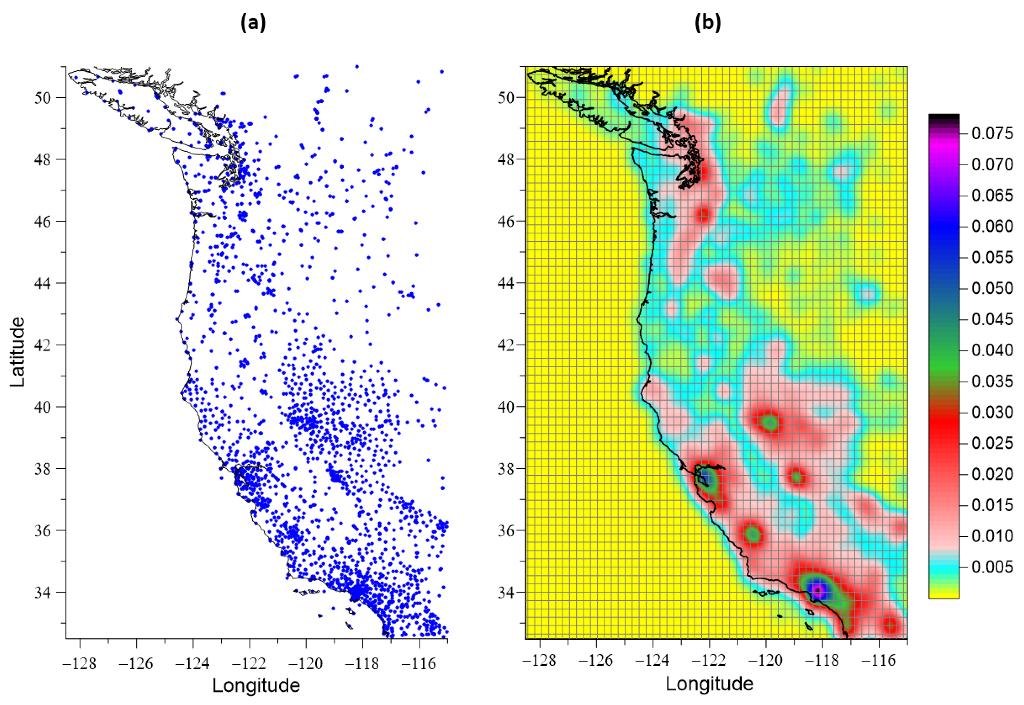
In what follows, we will consider a regular grid of 100 × 150 nodes, covering an area with latitude from 32.5° N to 51° N and longitude from 115° W to 128.5° W. Figure 1a shows the positions of GPS points for measuring displacements of the Earth’s surface. Figure 1b shows the distribution density of GPS stations obtained using the Gaussian kernel estimate [23] at the nodes of this regular grid with a smoothing radius of 0.25° (about 28 km).
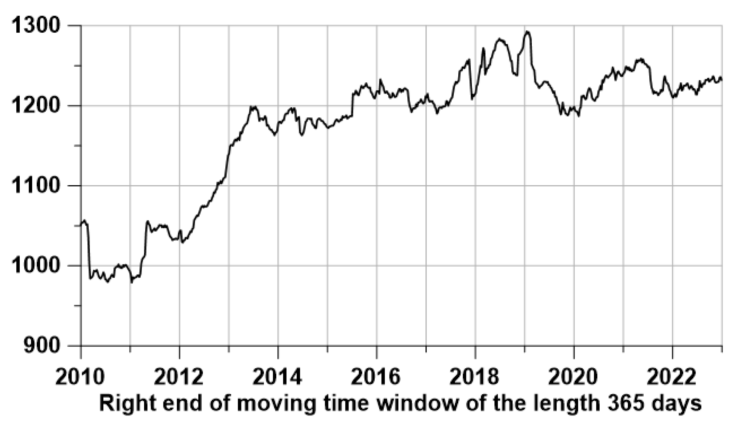
We will consider estimates of the properties of GPS time series in a moving time window 365 days long with a shift of 7 days. For each time window, operable stations are determined from the condition that the number of gaps in the considered time window does not exceed 5% of the time window length, that is, that this number is not more than 18 values. Missing values are filled in with artificial data, which are found from the value to the left and right of the missing time interval of the same length as the length of the gap [19]. Figure 2 shows a graph of the number of working stations within a sliding time window of 365 days for 14 years of observations, 2009–2022.
3. Description of the Time Series Statistics Used
For each station in each time window, four surface tremor statistics are computed for the three ground displacement components.
Spectral exponent. Let be a sample of the GPS time series within a window of sample lengths . Denote by the estimate of the signal power spectrum —a sequence of discrete values of frequencies with a step , , , —a time step. Here, is the minimum length, which is greater than or equal to the sample length : , the index in Formula (6) varies up to due to the symmetry of the power spectrum of real signals with respect to the Nyquist frequency : . We introduce the spectral exponent by the following formula:
where period , the value is determined by the least squares method: , is a sequence of random variables with zero mean. In each time window, the power spectrum was computed after transition to increments using an autoregressive model (maximum entropy estimate) [24] with an autoregressive order of , i.e., 36 for a window of length 365 samples. The transition to increments before calculating the power spectrum aims to free from the dominant effect of low frequencies in the daily time series of GPS.
We then address wavelet-based entropy and wavelet-based spectral slope. The minimum normalized wavelet information entropy for the sample is determined by the following formula:
Here, denotes the coefficients of the orthogonal wavelet decomposition. Daubechies bases were used with the number of vanishing moments from 1 to 10 [25]. We chose such a basis from this set for which the value (2) is minimal for a given time window and for the considered component of the displacement of the Earth’s surface. By Formula (2), .
For the orthogonal wavelet, which is found from a minimum of entropy, the wavelet power spectrum can be calculated as the average values of the squares of the wavelet coefficients at each level of detail of the decomposition:
In Formula (3), are the wavelet coefficients at the detail level with number , index , where is the number of wavelet coefficients at the detail level with number , which corresponds to the frequency band with the central period [25]. The maximum detail level number is chosen such that it contains at least a given number of wavelet coefficients. Recall that the number of wavelet coefficients at the level of detail decreases by a factor of 2 when the level number increases by one. The value was used in the calculations, which gives the value for the window length . Values , are similar to conventional power spectra. The regression model is used to calculate the wavelet-based spectral slope:
where is a sequence of random variables with zero mean. The parameter in Formula (4) is the wavelet-based spectral exponent, the value of which can be found by the least squares method: .
We then address the Donoho–Johnstone index (DJ-index). The threshold is defined by the following formula [25,26]:
The threshold (5) separates rather large (informative), in their absolute values, wavelet coefficients from other coefficients which are considered to be noisy. Thus, we can consider the dimensionless signal characteristics , , as the ratio of the number of the largest wavelet coefficients, for which the inequality is fulfilled, to the number N of all wavelet coefficients.
The value in the Formula (5) is the noise standard deviation estimate under the assumption that the noise is most concentrated in the first-detail level of orthogonal wavelet decomposition. The estimate of standard deviation should be robust with respect to outliers in the values of the coefficients at the first level. To provide this, a median estimate of the standard deviation for a normal random variable is used:
For each station in each time window, four surface tremor statistics are computed for the three ground displacement components where ck(1) are wavelet coefficients at the first level of detail. The estimate of the standard deviation σ from Formula (6) determines the value (5) as a threshold for extracting noise wavelet coefficients. The quantity (5) is known in wavelet analysis as the Donoho–Johnstone threshold, and the expression for this quantity is based on the formula for the asymptotic probability of the maximum deviations of Gaussian white noise [25,26]. The DJ index values can be interpreted as a measure of the non-stationarity of seismic noise. For stationary Gaussian white noise, the index is zero. In [27,28], the DJ index was used as one of the main statistics for investigating properties of global seismic noise.
In summary, we will briefly describe in the list the characteristics of the values of the tremor statistics for stationary white Gaussian noise, which is considered as a standard of a completely random oscillation:
- The “usual” spectral exponent is the coefficient of regression between the logarithm of the power spectrum values and the logarithm of the period (“spectral slope”). For white noise, it is equal to zero (white noise has a “flat spectrum”).
- Wavelet-based spectral exponent —the regression coefficient between the logarithm of the mean values of the squared wavelet coefficients for each level of detail and the logarithm of the period of the central frequency corresponding to the level of detail of the wavelet decomposition (“spectral slope”). For white noise, it is zero.
- Donoho–Johnstone threshold (DJ index) —the ratio of the number of “large” in absolute magnitude orthogonal wavelet coefficients to the total number of coefficients. For white noise, it is zero.
- Minimum entropy of the distribution of squared orthogonal wavelet coefficients in the enumeration of wavelet basis functions in the class of Daubechies wavelets with the number of vanishing moments from 1 to 10. For white noise, the entropy is maximum.
Since we use four statistics for three components of the ground displacement vector, we obtain 12 statistics for each type of tremor. Let us put them in one matrix:
On the left side of the matrix (7), there are the designations of the characteristics of active tremor, on the right side of the matrix (7) there are the designations of the characteristics of passive tremor. Recall that we are considering a regular grid of nodes with a size of 100 nodes in longitude and 150 nodes in latitude. For each time window with a length of 365 days with a shift of 7 days, the values of all 12 sequences of the distribution of tremor properties at the nodes of the regular grid are determined.
4. Extreme Value Probability Density Maps
Let be any value from the matrix (7), the estimates of which were obtained in a moving time window. For each grid node and for each time window labeled at the right end of the window, we find the 10 closest seismic working stations, which gives 10 values of . Let us take their median value . The values form an “elementary” map corresponding to a time window of 365 days. Consider the values of the parameter as a function of two-dimensional vectors of longitudes and latitudes of nodes in an explicit form: . For each “elementary map” with a discrete time index , we find the coordinates of the nodes at which the extreme value is reached with respect to all other nodes of the regular grid.
As noted above, the choice of the minimum for entropies and the maximum for spectral slopes is due to the considerations that the regions of active tremor should be characterized by the values of statistics that reflect the maximum deviation from the properties of white noise. For passive tremor, the opposite is true: maxima for entropies and minima for spectral slopes. A cloud of 2D vectors considered within a certain time interval composes some random set. Let us estimate two-dimensional probability density function for each node of the regular grid. For this, the Parzen–Rosenblatt estimate with the Gaussian kernel function [23] will be applied:
Here, is the averaging radius, integer indices enumerate the maps of each time window. The equals the number of time windows in the considered time interval. The width of the smoothing band was used, which is approximately equal to 28 km.
In our analysis, time windows of two lengths are used: a “short” window of 365 days in length, which is used to obtain estimates of tremor parameters, and a “long” window of 1095 days (3 years) in length, in which a sequence of estimates of the distribution densities of extreme values of statistics is the obtained tremor. Estimates of characteristics from matrix (7) are calculated using “short” time windows 365 days long. Next, the probability densities of extreme values are calculated from the values that fall within the current “long” time window of 1095 days, which are also shifted by 7 days. Each “long” window includes 105 “short” time windows.
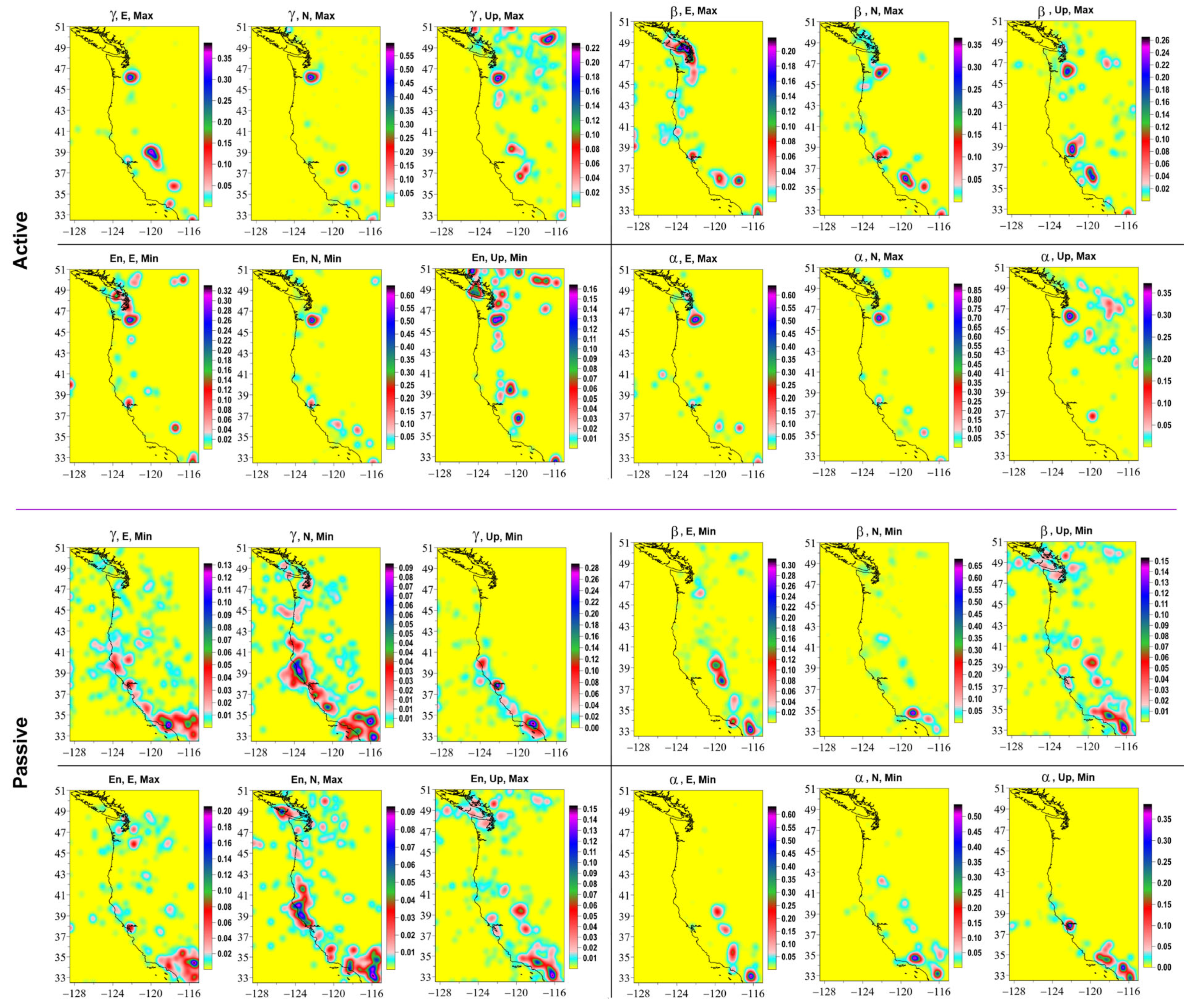
As a result of such assessments, 24 maps of the distribution density of extreme values of tremor parameters were constructed, presented in Figure 3, on which 12 maps for active tremor are in the upper half, and 12 maps for passive tremor are in the lower half.
Purely visually, a correlation of probability density maps of the distribution of extreme values of tremor statistics is noticeable. The principal component method [29] is used to extract the most common spatial characteristics. In each “long” 3-year time window, a correlation matrix of the size 12 × 12 between the probability densities of the distribution of extreme values of tremor statistics is calculated. The eigenvector corresponding to the maximum eigenvalue of the correlation matrix is found and the squares of its components were used as weights to calculate the average weighted probability density in each “long” window. The coordinates of the point that realizes the maxima of average density were found. These operations make it possible to obtain the trajectory of geographic coordinates of points that realize the maximum values of the average probability density. These points are called singular tremor points.
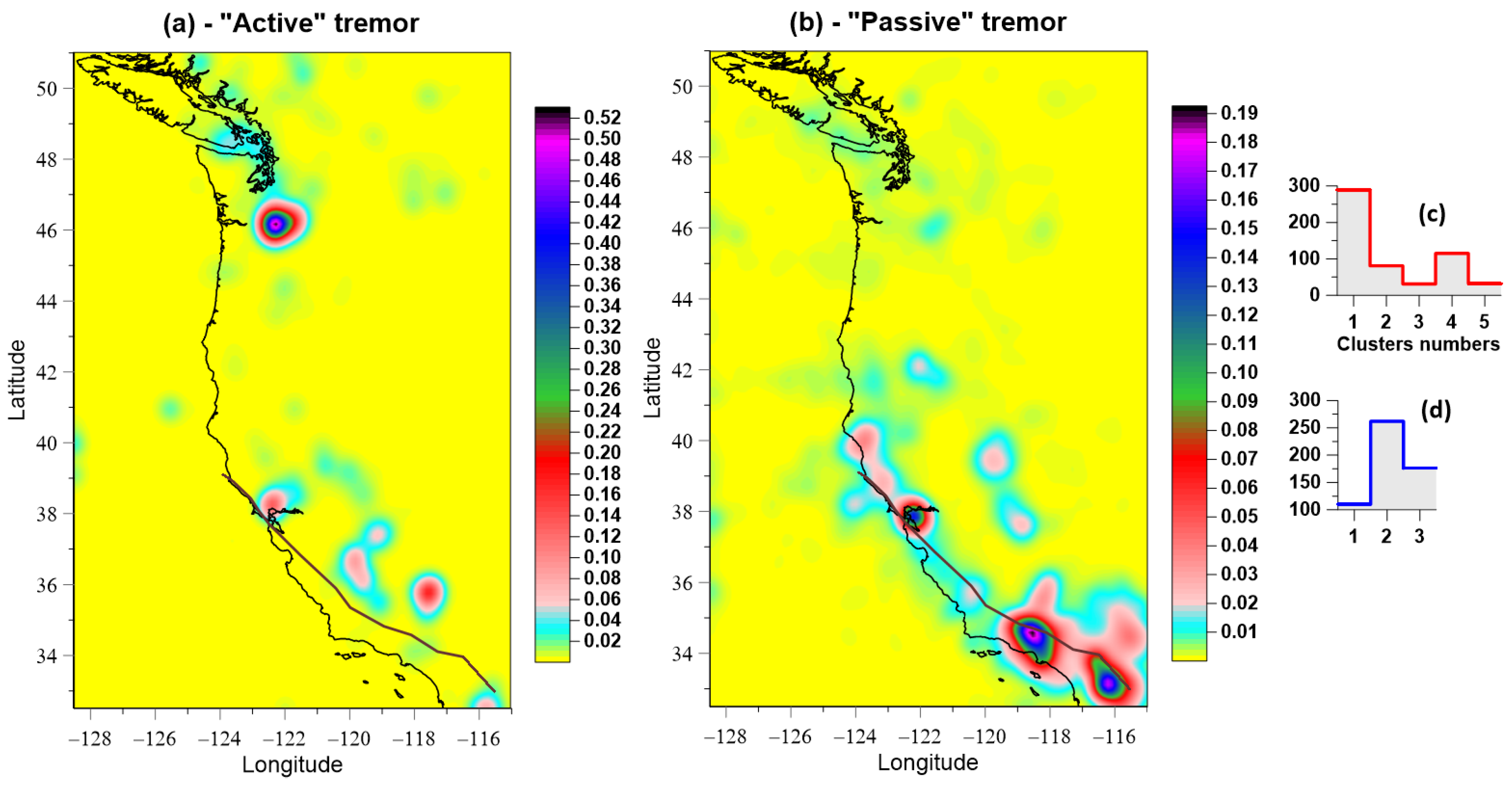
The results of weighting the probability density maps of the distribution of extreme properties of tremor by the method of principal components are shown in Figure 4. On Figure 4a, red circles indicate the positions of singular points of active tremor, which are combined into five clusters. The clusters are numbered in descending order of the latitude of their centers of mass: the cluster numbers are also shown. On Figure 4b, blue circles indicate the positions of singular points of passive tremor, which form three clusters. On Figure 4c,d, there are plots of histograms of the distribution of the number of singular points in each cluster for each type of tremor.
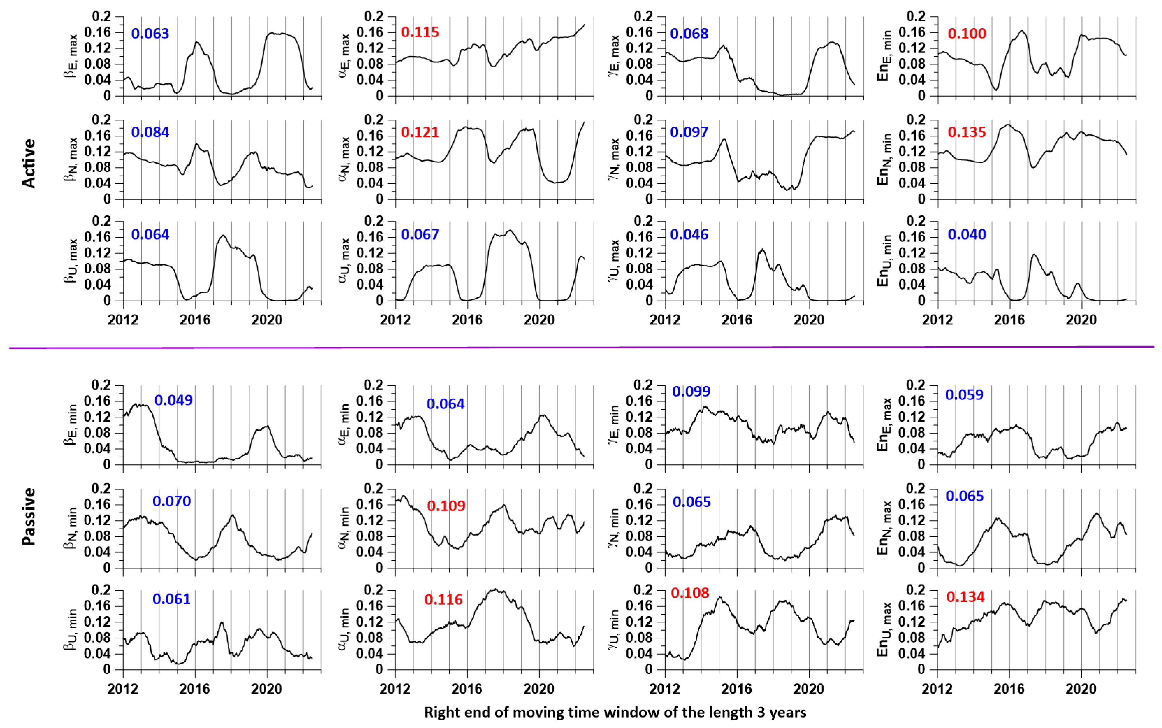
Figure 5 shows graphs of changes in the squares of the components of sequences of correlation matrices for probability density maps of the distribution of extreme values, respectively, for active (12 upper graphs) and passive (12 lower graphs). As noted above, these values are used as weight functions to obtain weighted average probability density maps. The result of such a weighing operation using the principal component method is shown in Figure 4. The graphs in Figure 5 show the average values of the weights calculated for all “long” time windows. For each tremor variant, four maximum average values of weights are highlighted in red—they select those components from matrix (7) that make the greatest contribution to obtaining the weighted average sum of probability densities.
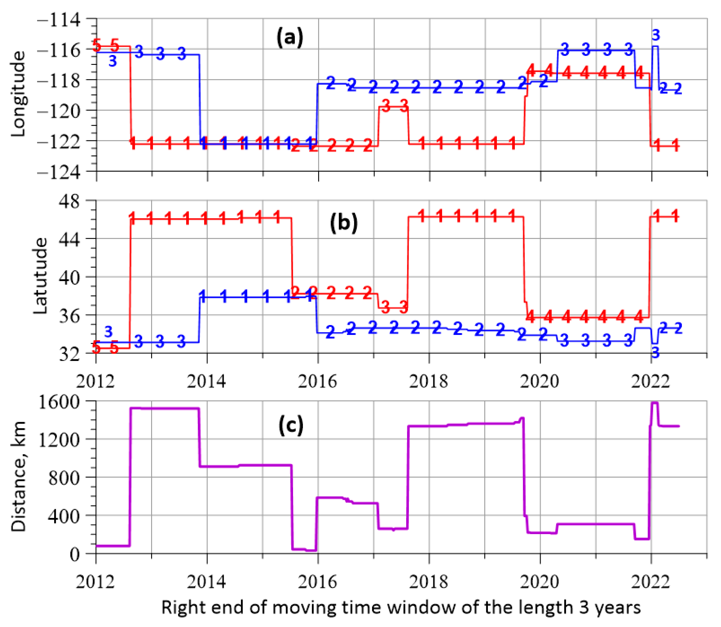
The trajectories of changes in geographic latitudes and longitudes of singular points over time are shown in Figure 6a,b. Along the trajectories of change of coordinates, there are marks of belonging to clusters of stations. Figure 6c shows how the distances between the singular points of active and passive tremor change as the time window of the length of 3 years moves from left to right. From this graph, it can be seen that the concentration of singular points of both types of tremor in those regions where their positions are very close to each other, namely cluster #2 of active singular points and cluster #1 of passive singular points mainly occur in different time windows. The exception is the time intervals with labels of the right ends of the “long” 3-year windows 2012–June 2012 and June 2015–2016, when the distances from singular points of different types are less than 100 km, but do not reach zero values.
As can be seen from Figure 4b, clusters of singular points of passive tremor are concentrated in the vicinity of three fragments of the San Andreas fault. At the same time, Figure 6 shows that there is a switching mode from one cluster to another with long time intervals of belonging to one or another cluster. A hypothesis can be proposed that this behavior reflects the modes of activation of chaotic movements of crustal blocks in these three fragments of the fault, which causes the properties of high-frequency surface movements to approach white noise.
As for the singular points of active tremor, their occurrence may be associated with the processes of consolidation of small blocks of the Earth’s crust and the formation of temporary larger structures that respond to external influences (such as atmospheric cyclones) with a greater amplitude, which, on the contrary, leads to an increase in the deviation from the properties of white noise.
Of particular interest are short time intervals of small distances between the singular points of active and passive tremor, which are visible in Figure 6c. They can highlight areas of the Earth’s crust that are in an unstable state.
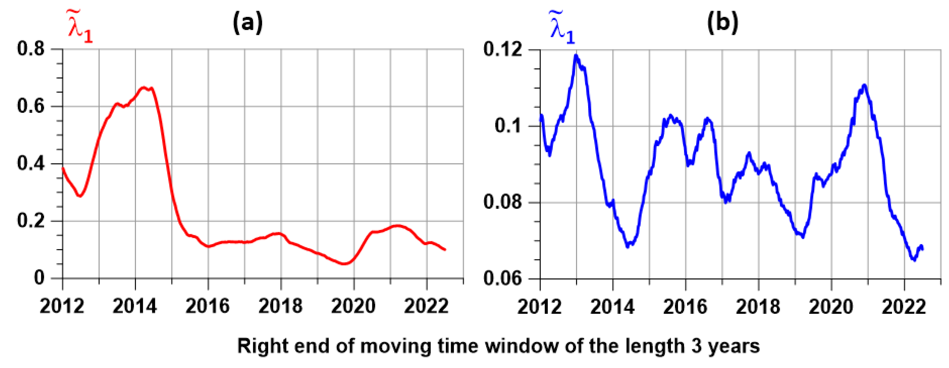
Let be the normalized maximum eigenvalue of the correlation matrix:
In Formula (9), are the eigenvalues of the correlation matrix, sorted in descending order: . According to the principal component method [29], the value is equal to the share of the total variance attributable to the first principal component and can be interpreted as a measure of synchronization of changes in the scalar components of the multivariate time series of the probability density values of the tremor statistics from the matrix in Formula (7) in regular grid nodes covering the region under study.
Figure 7 shows graphs of changes in the eigenvalues of the correlation matrix for active and passive tremor. It can be seen from these plots that the active tremor (Figure 7a) is much more synchronized than the passive tremor (Figure 7b). Moreover, for active tremor, there is a very strong synchronization for the positions of the right end of the 3-year time window from 2013 to 2015. Given the length of the window, this synchronization takes a period of time from 2010 to 2015.
As was shown in [28], after a couple of the strongest earthquakes in the world, Maule in Chile on 27 February 2010 and Tohoku in Japan on 3 November 2011, there was an explosive increase in the radius of spatial correlations of global seismic noise properties. It is possible that the increase in synchronization of active tremor in the western United States in 2010–2015 is also a response to this pair of mega earthquakes. Note that a sharp jump in the magnitude of global correlations of the Earth’s surface tremor in 2010–2011 was shown in [19].
5. Conclusions
A method has been proposed for studying the properties of the Earth’s surface tremor, measured by means of GPS, based on the use of oscillation statistics that describe the deviation or similarity to the properties of Gaussian white noise, considered as a standard of a stationary random signal. Based on the application of the principal component method to the estimation of the probability densities of the distribution of extreme properties of statistics in a moving time window, concepts of active and passive tremor and their singular points are introduced, and the trajectories of singular points are determined. The concept of tremor synchronization measure is introduced as the maximum eigenvalue of the correlation density matrix of distribution of extreme values of tremor statistics. The method is applied to the data of daily GPS time series on a network of stations located in California during the time interval 2009–2022. It was shown that singular points of both types of tremor form well-defined clusters. A hypothesis is proposed that the difference in the types of singular points of tremor is associated with different mechanisms of consolidation of crustal blocks. In particular, passive tremor may be due to the activation of chaotic block movements in the vicinity of three fragments of the San Andreas fault. Estimates of measures of synchronization of active and passive tremor are given. A hypothesis has been put forward that the strong synchronization of active tremor in 2010–2015 caused a jump in the global synchronization of the tremor of the Earth’s surface and an explosive increase in the correlations of global seismic noise in 2010–2011.
Funding
The work was carried out within the framework of the state assignment of the Institute of Physics of the Earth of the Russian Academy of Sciences (topic FMWU-2022-0018).
Institutional Review Board Statement
Not applicable.
Informed Consent Statement
Not applicable.
Data Availability Statement
The open access data from the source: http://geodesy.unr.edu/gps_timeseries/tenv3/IGS14/ (accessed on 1 May 2023) were used.
Conflicts of Interest
The author declare no conflict of interest.
References
- Roncagliolo, P.A.; Garcнa, J.G.; Mercader, P.I.; Fuhrmann, D.R.; Muravchik, C.H. Maximum-likelihood attitude estimation using GPS signals. Digit. Signal Process. 2007, 17, 1089–1100. [Google Scholar] [CrossRef]
- Wang, F.; Li, H.; Lu, M. GNSS Spoofing Detection and Mitigation Based on Maximum Likelihood Estimation. Sensors 2017, 17, 1532. [Google Scholar] [CrossRef]
- Parkinson, B.W. Global Positioning System: Theory and Applications; AIAA: Reston, VA, USA, 1996. [Google Scholar]
- Xu, J.; He, J.; Zhang, Y.; Xu, F.; Cai, F. A Distance-Based Maximum Likelihood Estimation Method for Sensor Localization in Wireless Sensor Networks. Int. J. Distrib. Sens. Netw. 2016, 12, 2080536. [Google Scholar] [CrossRef]
- Agnew, D. The time domain behavior of power law noises. Geophys. Res. Lett. 1992, 19, 333–336. [Google Scholar] [CrossRef]
- Amiri-Simkooei, A.R.; CTiberius, C.J.M.; Teunissen, P.J.G. Assessment of noise in GPS coordinate time series: Methodology and results. J. Geophys. Res. 2007, 112, B07413. [Google Scholar] [CrossRef]
- Bos, M.S.; Fernandes, R.M.S.; Williams, S.D.P.; Bastos, L. Fast error analysis of continuous GPS observations. J. Geod. 2008, 82, 157–166. [Google Scholar] [CrossRef]
- Kermarrec, G.; Schon, S. On modelling GPS phase correlations: A parametric model. Acta Geod. Geophys. 2018, 53, 139–156. [Google Scholar] [CrossRef]
- Liu, B.; Xing, X.; Tan, J.; Xia, Q. Modeling Seasonal Variations in Vertical GPS Coordinate Time Series Using Independent Component Analysis and Varying Coefficient Regression. Sensors 2020, 20, 5627. [Google Scholar] [CrossRef]
- Tesmer, V.; Steigenberger, P.; van Dam, T.; Mayer-Gurr, T. Vertical deformations from homogeneously processed GRACE and global GPS long-term series. J. Geod. 2011, 85, 291–310. [Google Scholar] [CrossRef]
- Yan, J.; Dong, D.; Burgmann, R.; Materna, K.; Tan, W.; Peng, Y.; Chen, J. Separation of Sources of Seasonal Uplift in China Using Independent Component Analysis of GNSS Time Series. J. Geophys. Res. Solid Earth 2019, 124, 11951–11971. [Google Scholar] [CrossRef]
- Pan, Y.; Shen, W.-B.; Ding, H.; Hwang, C.; Li, J.; Zhang, T. The Quasi-Biennial Vertical Oscillations at Global GPS Stations: Identification by Ensemble Empirical Mode Decomposition. Sensors 2015, 15, 26096–26114. [Google Scholar] [CrossRef] [PubMed]
- Liu, B.; Dai, W.; Liu, N. Extracting seasonal deformations of the Nepal Himalaya region from vertical GPS position time series using Independent Component Analysis. Adv. Space Res. 2017, 60, 2910–2917. [Google Scholar] [CrossRef]
- Santamarнa-Gymez, A.; Memin, A. Geodetic secular velocity errors due to interannual surface loading deformation. Geophys. J. Int. 2015, 202, 763–767. [Google Scholar] [CrossRef]
- Fu, Y.; Argus, D.F.; Freymueller, J.T.; Heflin, M.B. Horizontal motion in elastic response to seasonal loading of rain water in the Amazon Basin and monsoon water in Southeast Asia observed by GPS and inferred from GRACE. Geophys. Res. Lett. 2013, 40, 6048–6053. [Google Scholar] [CrossRef]
- Chanard, K.; Avouac, J.P.; Ramillien, G.; Genrich, J. Modeling deformation induced by seasonal variations of continental water in the Himalaya region: Sensitivity to Earth elastic structure. J. Geophys. Res. Solid Earth 2014, 119, 5097–5113. [Google Scholar] [CrossRef]
- He, X.; Montillet, J.P.; Fernandes, R.; Bos, M.; Yu, K.; Hua, X.; Jiang, W. Review of current GPS methodologies for producing accurate time series and their error sources. J. Geodyn. 2017, 106, 12–29. [Google Scholar] [CrossRef]
- Ray, J.; Altamimi, Z.; Collilieux, X.; van Dam, T. Anomalous harmonics in the spectra of GPS position estimates. GPS Solut. 2008, 12, 55–64. [Google Scholar] [CrossRef]
- Lyubushin, A. Global coherence of GPS-measured high-frequency surface tremor motions. GPS Solut. 2018, 22, 116. [Google Scholar] [CrossRef]
- Lyubushin, A. Field of coherence of GPS-measured earth tremors. GPS Solut. 2019, 23, 120. [Google Scholar] [CrossRef]
- Lyubushin, A. Identification of Areas of Anomalous Tremor of the Earth’s Surface on the Japanese Islands According to GPS Data. Appl. Sci. 2022, 12, 7297. [Google Scholar] [CrossRef]
- Blewitt, G.; Hammond, W.C.; Kreemer, C. Harnessing the GPS data explosion for interdisciplinary science. Eos 2018, 99, 485. [Google Scholar] [CrossRef]
- Duda, R.O.; Hart, P.E.; Stork, D.G. Pattern Classification; Wiley: Hoboken, NJ, USA, 2000. [Google Scholar]
- Marple, S.L., Jr. Digital Spectral Analysis with Applications; Prentice-Hall, Inc.: Englewood Cliffs, NJ, USA, 1987. [Google Scholar]
- Mallat, S. A Wavelet Tour of Signal Processing, 2nd ed.; Academic Press: Cambridge, MA, USA, 1999. [Google Scholar]
- Donoho, D.L.; Johnstone, I.M. Adapting to unknown smoothness via wavelet shrinkage. J. Am. Stat. Assoc. 1995, 90, 1200–1224. [Google Scholar] [CrossRef]
- Lyubushin, A. Low-Frequency Seismic Noise Properties in the Japanese Islands. Entropy 2021, 23, 474. [Google Scholar] [CrossRef]
- Lyubushin, A. Spatial Correlations of Global Seismic Noise Properties. Appl. Sci. 2023, 13, 6958. [Google Scholar] [CrossRef]
- Jolliffe, I.T. Principal Component Analysis; Springer: Berlin/Heidelberg, Germany, 1986. [Google Scholar]
Figure 1.
(a) Network of GPS stations (blue dots) in the US West, 2009–2022; (b) the density of GPS stations, estimated using a Gaussian kernel with a smoothing radius of 0.25 degrees on a regular grid of nodes with a size of 100 × 150. Plot (b) presents every second grid line by coordinates, because all the grid lines form too dense a network.

Figure 2.
The number of operational GPS stations in a window of the length 365 days with mutual shift of 7 days.
Figure 2.
The number of operational GPS stations in a window of the length 365 days with mutual shift of 7 days.

Figure 3.
Average probability densities of distribution of extreme values of 4 statistics of “active” and “passive” tremor of the Earth’s surface for 3 components of the displacement vector. Due to the fact that each property value is estimated over a 365-day window offset by 7 days, the average probability density estimate is obtained by averaging 548 probability density maps, each derived from 105 tremor property value maps.

Figure 4.
(a,b) are the results of averaging the weighted average probability densities of extreme values of 12 surface tremor parameters over a moving time window of 3 years for active and passive tremor. The red circles in (a) represent the positions of active tremor singular points forming 6 numbered clusters, the blue circles in (b) represent the positions of passive tremor singular points forming 3 numbered clusters. Bold brown line presents San Andreas fault. (c,d) are histograms of the numbers of singular points for “active” and “passive” tremors belonging to different clusters.

Figure 5.
Plots of changes in the weights of each of the 12 probability densities in “long” time windows of 1095 days with a shift of 7 days for “active” and “passive” tremor. The numbers indicate the average values of the weights, the 4 largest averages out of 12 variants for each type of tremor are highlighted in red, other values are highlighted by blue.

Figure 6.
(a,b) represent time sequences of longitudes and latitudes of singular points of tremor with a shift in the time window of 3 years for “active” (red) and “passive” (blue) tremor with cluster membership marks. (c) is the distance between the singular points of active and passive tremor in each time window of 3 years. Numbers along red and blue lines indicate the numbers of the active and passive tremor clusters to which belong the current point of the trajectory. There are time intervals when longitude and latitude trajectories of singular points for different types of tremor are very close to each other.

Figure 7.
(a,b) represent time sequences of values of the normalized maximum eigenvalue of the correlation matrix with a shift in the time window of 3 years for “active” (a) and “passive” (b) tremor.
Figure 7.
(a,b) represent time sequences of values of the normalized maximum eigenvalue of the correlation matrix with a shift in the time window of 3 years for “active” (a) and “passive” (b) tremor.

Disclaimer/Publisher’s Note: The statements, opinions and data contained in all publications are solely those of the individual author(s) and contributor(s) and not of MDPI and/or the editor(s). MDPI and/or the editor(s) disclaim responsibility for any injury to people or property resulting from any ideas, methods, instructions or products referred to in the content. |
© 2023 by the author. Licensee MDPI, Basel, Switzerland. This article is an open access article distributed under the terms and conditions of the Creative Commons Attribution (CC BY) license (https://creativecommons.org/licenses/by/4.0/).
Share and Cite
MDPI and ACS Style
Lyubushin, A. Singular Points of the Tremor of the Earth’s Surface. Appl. Sci. 2023, 13, 10060. https://doi.org/10.3390/app131810060
AMA Style
Lyubushin A. Singular Points of the Tremor of the Earth’s Surface. Applied Sciences. 2023; 13(18):10060. https://doi.org/10.3390/app131810060
Chicago/Turabian StyleLyubushin, Alexey. 2023. "Singular Points of the Tremor of the Earth’s Surface" Applied Sciences 13, no. 18: 10060. https://doi.org/10.3390/app131810060
Note that from the first issue of 2016, this journal uses article numbers instead of page numbers. See further details here.