Abstract
During an optimization process which uses a metaheuristic strategy applied to the nesting problem, it is required to apply a repair method if the random solution contains overlapping items. In this paper, a repair method is proposed to avoid the overlap of pixels between items obtained by a randomly generated solution using metaheuristics. The proposed procedure runs through each one of the items. When it finds at least one overlapping pixel, it performs four moves: up, down, left, and right, and it is repeated until no more overlaps appear. In addition, a structure called muéganos is defined. It contains items that are nested more compactly to minimize waste. This structure allows the nesting of elements in a more efficient way. To complete the procedure, a sequential greedy algorithm (SGA) was implemented to nested the items in the available area of the material. A comparison was made between nesting without and with muéganos, obtaining better results using muéganos, with a material utilization of more than . From the experimental results, it was obtained that the solutions are improved by more than through our proposed method, which is competitive when compared to other methods proposed in the literature.
1. Introduction
The nesting of items in finite materials is a combinatorial optimization problem to be solved in a significant number of manufacturing industries, such as metallurgical, paper, textile, footwear, and glass. Optimal nesting is essential for the best use of the materials and to minimize waste through the use of Computer Vision, Computational Intelligence and Digital Image Processing techniques [1].
Heuristic and metaheuristic methods [2,3] can be applied to complex optimization problems, such as the nesting problem, to approximate solutions. These methods guide the search process by approximating optimal solutions. Some examples of metaheuristic algorithms include greedy algorithms [4,5,6], simulated annealing (SA) [7], particle swarm optimization (PSO) [8,9], and genetic algorithms (GAs) [10,11,12,13]. Simulated annealing (SA) [7] is a probabilistic algorithm that approximates the global optimum by allowing some suboptimal moves. SA is a stochastic optimization method [14] based on the principles of statistical mechanics. It simulates the annealing process by slowly cooling a substance to obtain a strong crystalline structure. The strength of the structure depends on the cooling rate of the metals. SA can be used to approximate global solutions in an extended space search for an optimization problem.
Greedy algorithms [4,5,6] make local optimal choices at each step, which can lead to suboptimal solutions. Particle swarm optimization [8,9] is a metaheuristic optimization algorithm inspired by simulating the behavior of a swarm of particles observed in nature, such as fish, birds, and ants, among others.
GAs are one of the most popular techniques among evolutionary algorithms. They were inspired by Darwin’s theory of evolution [11] on the basis of the principle of natural selection. GAs were implemented by John Holland, a researcher at the University of Michigan, in the late 1960s [13]. GAs are stochastic search strategies based on the natural selection mechanism since they involve aspects of natural genetics, imitating biological evolution as a search strategy to solve problems [10]. GAs have three significant advantages in optimization problems: adaptability, robustness, and flexibility [15].
Related Work
Despite the methods and techniques developed to automate the nesting process, many industries still perform the procedure manually, which results in a substantial waste of material and time while performing the procedure. Some studies focused on the nesting problem are mentioned. Yi-Ping Cui et al. [16] implemented an algorithm that produces patterns from items using a sequential heuristic procedure. A pattern contains three items, which are produced from a greedy algorithm that organizes them using the left-bottom algorithm, and generates a position from the corners of the first pattern to place them in a specific orientation (vertical or horizontal). After the generation, the item values are adjusted using a value correction formula. Defu Zhang et al. [17] proposed a recursive technique to solve nesting problems by dividing the material into areas and assigning priorities to each item. These priorities depend on its size to efficiently fill the rectangle where it is placed.
Gomez and Terashima-Marín [18] used an evolutionary framework to build hyperheuristics that solve the nesting problem, which considers the minimization of two objectives: the number of items to be accommodated and the time needed for this task. It also integrates three multi-objective evolutionary algorithms that build a solution, and decides which of the three solutions is the best at each algorithm step. Leung et al. [19] presented a two-stage intelligent search algorithm for a two-dimensional strip packing problem. First, a heuristic algorithm selects a rectangular item from all items to be nested for a given space. Second, a local search and a simulated annealing algorithm are combined to enhance the solutions to the problem.
Neuenfeldt Júnior et al. [20] explored benchmark values (predictors) for the optimal objective function of hard combinatorial optimization problems based on mining techniques, which can be used to evaluate the quality of heuristic solutions for the 2D nesting problem. Wei et al. [6] presented a method based on the branch-and-bound best-fit ladder to solve this problem. Moreover, a greedy heuristic is used to accelerate the process and generate a complete solution from a partial one. Yin, A. H., et al. [21] proposed a Quick Heuristic-Dynamic Programming (QHDP) algorithm. At the beginning, a one-dimensional knapsack problem creates sets as a function of the height and width of small rectangular blocks, and an efficient discretization set is generated for each one. Then, each set value is used as a possible cut-off line coordinate for the subproblem division. Pinheiro et al. [22] presented a shrinking algorithm that operates within a random-key genetic algorithm (RKGA) and well-known collocation rules (e.g., bottom-left) to improve partial solutions.
Rashid, D.N.H, et al. [23] designed the Ants Nesting method (ANA), inspired by Leptothorax ants, which emulates the behavior of ants searching for positions to deposit grain while building a new nest. ANA is a continuous algorithm that updates the search agent position by adding the rate of change: step or velocity. It calculates the rate of change differently as it uses the current and previous solutions and fitness values to generate weights during the optimization process. The Pythagorean theorem is used to obtained the weights, which lead the search agents during the exploration and exploitation phases.
It is possible to consider machine learning algorithms to solve the nesting problem; for example, a neural network can be integrated into image processing as in the research of Ding et al. [24], which presented a fuzzy image-enhancement method that can be applied to image processing at the initial stage to solve the nesting problem. Zhang and Ding et al. [25] proposed to transform the extracted features using a trained self-supervised feature extractor to reduce the mis-match in the feature distribution. Poshyanonda and Dagli [26] proposed a genetic algorithm to generate a sequence of patterns and use an allocation algorithm to place the sequence using a sliding method integrated with a neural network.
In the nesting problem, it is important to address the issue of overlaps between items. To avoid overlaps, it is required to apply techniques such as the repair of unfeasible solutions or the no-fit raster concept to check overlapping between any two-dimensional generic-shaped items. Mundim et al. [27] used the no-fit raster concept, which is used to check overlaps between any two-dimensional items in a generic way. They also implement a biased random-key genetic algorithm (BRKGA) to determine the sequence in which these items are packed. Once the sequence is obtained, they propose two heuristics based on the bottom-left movements and the no-fit raster concept, which are used to sort these items in the given container by observing objective criteria.
Kierkosz and Luczak [28] proposed a one-pass heuristic, placing items at different positions in the material to avoid the overlaps using the no-fit polygon (NFP) technique, thus generating different partial solutions, until the best one was found. Details of the NFP algorithm are found in [29]. Fischetti et al. [4] used a greedy strategy by applying a Mixed-Integer Programming (MIP) model for the nesting problem. Sato et al. [30] proposed an adaptation of the no-fit polygon to consider the penetration depth of the items. It is based on an iterative compaction scheme using a separation algorithm based on a fast obstruction map local search (FOMLS).
Repair algorithms are essential to improve and avoid overlapping items in the nesting problem. These algorithms can be developed using a greedy or random repair approach or a metaheuristic strategy to find feasible solutions. However, eliminating overlapping items is not the most effective solution as it can lead to more waste material. There are several possible methods to repair an individual that is not a feasible solution. Thomas Bäck et al. [31] explained that one of these methods is to create a repaired version that is a local solution for that particular individual. This repaired version can replace the original individual in the population under some probability. The repair of an unfeasible individual is related to learning and evolution, which interact with each other to improve and find a repaired and feasible solution called the Baldwin effect [32].
The contributions and innovations of this paper are summarized as follows:
- 1.
- A proposed repair method can be applied in a wide range of heuristic and metaheuristic techniques for solution approximation to solve the nesting problem.
- 2.
- A calibration method to enhance the measurement and scaling of items and material for the nesting process.
- 3.
- Enhanced efficiency and waste reduction through the use of muéganos as an innovative concept.
- 4.
- The muégano structure facilitates nesting of elements in a more compact form and minimizing waste.
- 5.
- Local optimization derived from the formation and optimal position of muéganos.
- 6.
- The sequential greedy algorithm (SGA) allows filling the available areas in the material with random pattern selection.
- 7.
- Improved application of metaheuristic algorithms when working with chromosomes or repaired solutions (e.g., genetic algorithms).
- 8.
- Experimental results underscore that the proposed method, particularly incorporating muéganos, leads to improved waste reduction and solution quality compared to previous methodologies.
The paper is structured as follows:
- Methodology: The procedure used to solve the nesting problem is explained, including the repair method proposed.
- Experimental Results: The results obtained with the proposed methodology are presented.
- Conclusions and future work: The conclusions drawn from the results are discussed, and suggestions for future work are provided.
2. Methodology
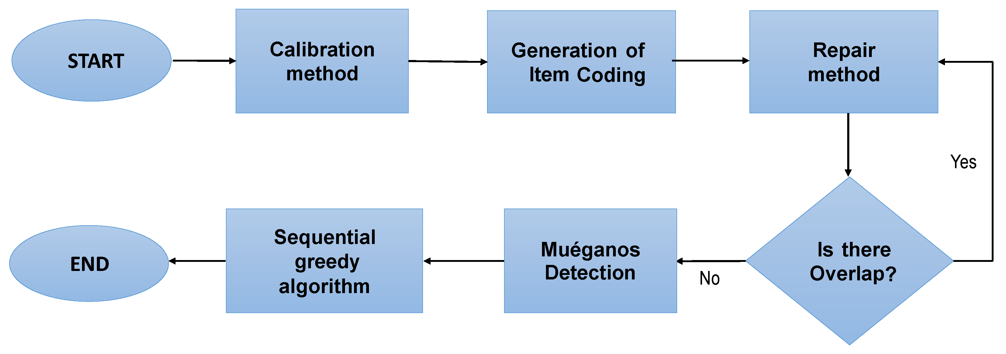
This article proposes a repair method that aims to minimize material waste by removing the least amount of elements from the nesting solution. Additionally, to improve the nesting between items, a structure called muéganos is proposed. It stores elements that have a limit of adjacent neighboring pixels between items. The objective of muéganos is to obtain the items closest to each other and then repeat them in nesting. Finally, a greedy sequential algorithm (SGA) was implemented to fill the available spaces in the material. Figure 1 shows the flow diagram of the repair process described in the methodology.

Figure 1.
Flow diagram of the repair process described in the methodology section. The process is a sequential flow starting with the camera calibration method to obtain the correct coordinates. Subsequently, the items are codified to apply the repair method. The muéganos are created from non-overlapping and low-waste items. Finally, the greedy algorithm optimizes the results.
2.1. Image Selection and Binarization
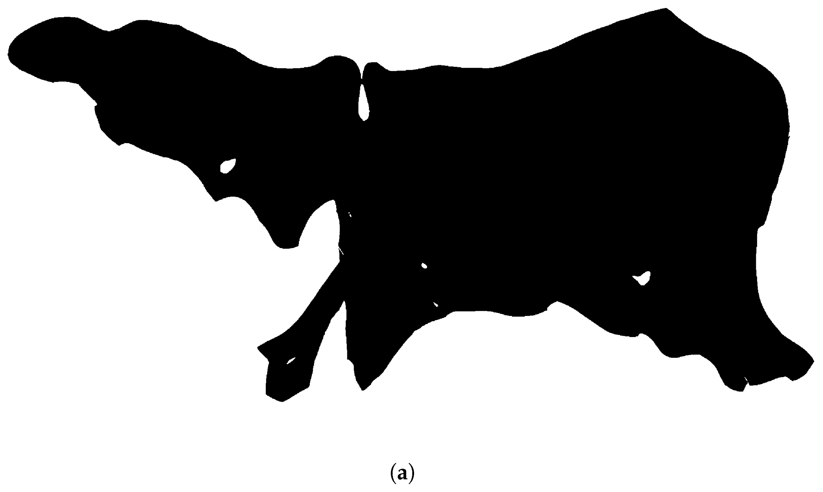
Firstly, the material and items are selected, and a binarization process is carried out using the OTSU method [33]. The valid area of the material and the items are binarized with values 0 and 1, respectively, and the invalid area (defects or holes) are given another value different from 0 and 1. The images stored in a data structure in conjunction with the area of each one are calculated by counting the number of valid pixels that are part of the nesting. Examples of binarized images are shown in Figure 2.

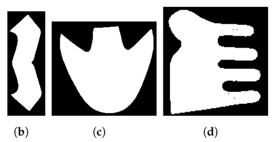
Figure 2.
Binarized material and items. (a) Sample cowhide material to accommodate items. (b–d) Footwear items nesting in the sample material.
Once all the items have been binarized, a bubble sorting algorithm is applied [34], to order them from the largest to the smallest area. When arranging them, they are packed with the largest area until the smallest one is arranged.
2.2. Calculation of Waste in Metric Values
Material and item images are scaled from the original frame size using a factor scale for reducing the material and the items. The pixel coordinates are transformed into world coordinates for a real-world application. This process implies a camera calibration method [35] and direct linear transformation (DLT) [36].
Firstly, the camera is calibrated using a set of C chessboard images from different perspectives. A checkerboard image is a grid with alternating black and white squares. The grid is used to show the size of the squares in metric and pixel dimensions. The camera calibration provides the intrinsic parameters (Equation (1)), such as focal length and optical center, and distortion parameters (Equation (2)), such as the radial and tangential distortion coefficients. The camera calibration helps to reduce the distortion in the images. Table 1 shows the variables corresponding to this section.

Table 1.
Calibration variables resume.
Once the camera parameters and distortion coefficients are obtained, the camera is fixed to a certain distance from the material. This arrangement makes it possible to obtain the transformation from 3D coordinates to 2D coordinates. This mapping is represented as
where represents the projection matrix, is the i-th 2D coordinate, and represents the i-th 3D coordinate for all , and n is the number of necessary points.
A chessboard is placed over the material, and the arrangement is captured. The arrangement is shown in Figure 3. Each corner of the physical chessboard is matched with the corresponding pixels.
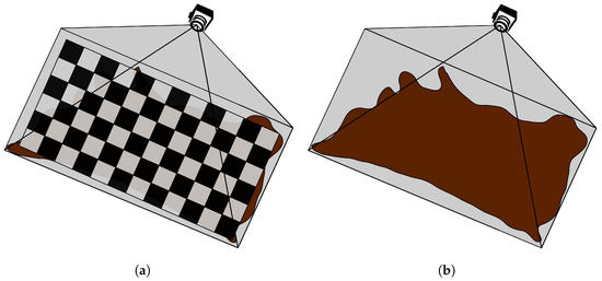
Figure 3.
Image (a) shows a chessboard pattern over the material. The chessboard should cover most of the material for the best calibration. In image (b), the camera captures the material for the nesting process.
The projection matrix used to transform the 2D coordinates to 3D coordinates is calculated as
Lastly, the parameters are obtained using the SVD method. Equation (4) is obtained from Equation (3).
The waste is calculated by selecting a rectangle around the material. The area of the rectangle is computed in pixels and meters. The ratio r of waste in pixels and the pixel area are equivalent to meters and metric area, as shown in Equation (5).
where is found as Equation (6):
The waste of the material in meters is calculated after the arrangement of patterns over the material.
2.3. Item Coding
Item coding is arranged as a data structure where all data items are stored. It is composed of individuals that are encoded as possible solutions to the nesting problem, which in most cases have overlapping. It is necessary to establish restrictions (Section 2.3.1) that guide the search process from the beginning of the algorithm. Table 2 describes the variables contained in item coding.
Table 2.
Variables for characterization of items involved in the constraints.
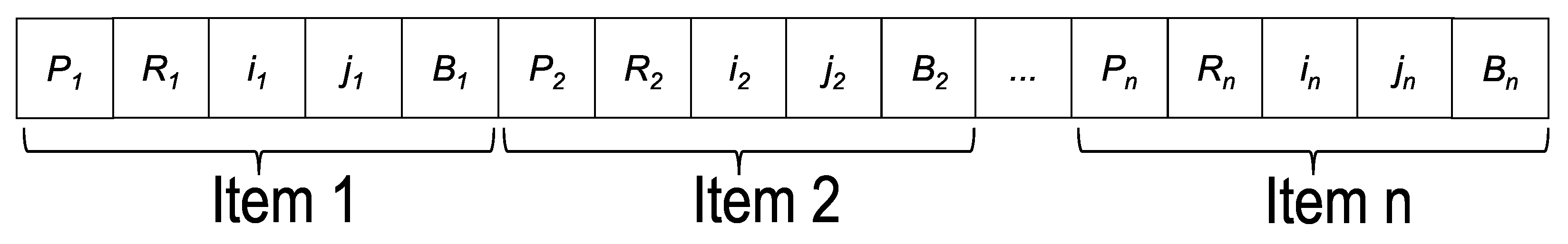
The item coding size defines the number of individuals or solutions generated by the algorithm, as shown in Figure 4.
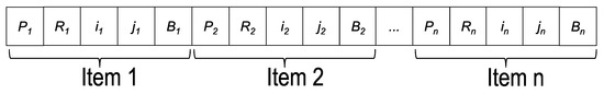
Figure 4.
Item coding contains all the items of the nesting. Each item is represented by five alleles: identifier (), rotation angle (), position in rows and columns within the material (,), and packing item ().
Each item is identified by five alleles as shown in Table 3.
Table 3.
Alleles identifying each item.
Packing item () identifies whether the allele is packaged or unpacked. If the item is packed, then it is not packed. In our case, when generating the item coding, all were considered with a value of 1 per item. The structure size is n, which defines the number of items that will be packed. k is an index of the number of items placed in position (,), where k is in the range of .
2.3.1. Restrictions on the Item Coding
When generating the item coding, the following restrictions are considered:
- 1.
- The positions in rows and columns must fall within the valid area of the material.
- 2.
- The percentage of pixels () outside the valid area () must allowed between items.
To define the positions of the rows and columns of each item, it is verified that the randomly generated values are within the valid area of the material, taking into account that only a percentage () of pixels outside the valid area are allowed, as shown in Equations (7) and (8):
where and are the numbers of rows and columns of the material, respectively, and and are the numbers of rows and columns of the item, respectively. The restrictions allow us to guide the search within a valid space from the beginning of the algorithm.
2.4. Repair Method
The repair method works on the solutions obtained from the applied metaheuristics. It goes through each item and performs four movements (up, down, left, and right) when overlaps are found. This process is repeated until there are no overlaps between items. If the number of overlapped pixels at the beginning is equal to the number of overlapped pixels after performing the movements, then the repair process stops. If there are overlapping items at the end, they are removed. The pseudocode for this process is shown in Algorithm 1.
| Algorithm 1: Repair Method |
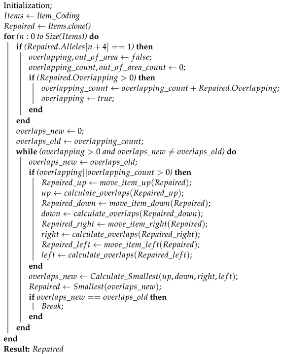 |
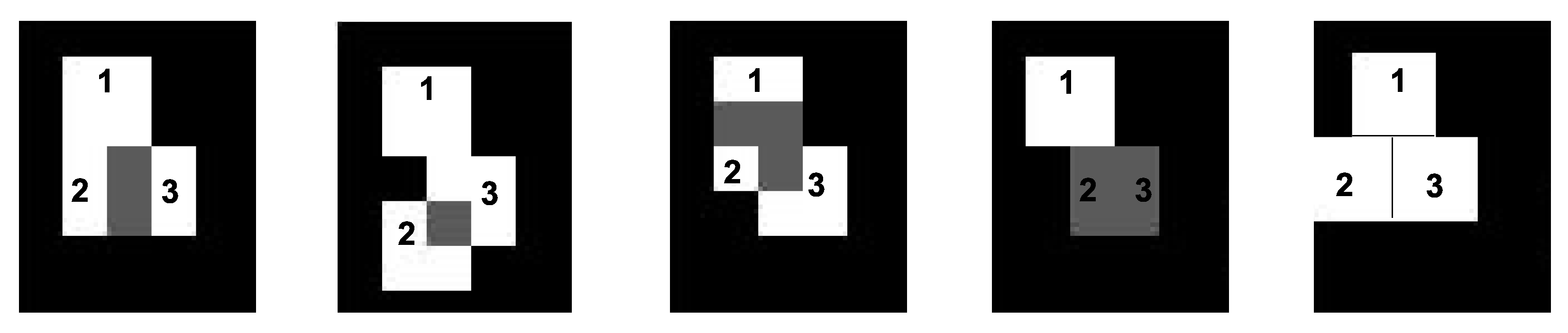
Figure 5 shows an example of how the item movements are carried out. There are 3 elements to nest, in which, item 2 is overlapped with item 3. Movements are made from left to right: down, up, right and left, and once the four movements have been made, the number of overlapped pixels is calculated. Then the left-movement-generated zero overlaps; therefore, we keep that solution. If there were overlaps in the first iteration, we would keep the smallest solution and repeat the process until the number of overlaps became zero.

Figure 5.
Sample of the item movements during the repair process. The black area represents the material, the white area represents the items, and the gray area represents the overlaps.
2.5. Muéganos Detection and Structure
In Mexico, the muégano is a candy that physically looks like several pieces of pastry stuck together with honey or caramel. Once it hardens, it is very difficult to separate them. The name muégano is also used with a social connotation to name a conglomerate of two or more people united by a strong bond.
The concept of muéganos can be applied in the repair process so that the patterns can be nested as much as possible and be arranged in a structure. Each muégano represents a list of items that have adjacent neighboring pixels; this means that if two items are joined by a limited number of pixels, then a muégano has been formed.
The Flood Fill Algorithm 2 was applied to detect the muéganos.The algorithm receives an image containing the repaired solutions. When it finds a contiguous pixel between items, those are labeled with a gray level.
| Algorithm 2: Flood Fill Algorithm |
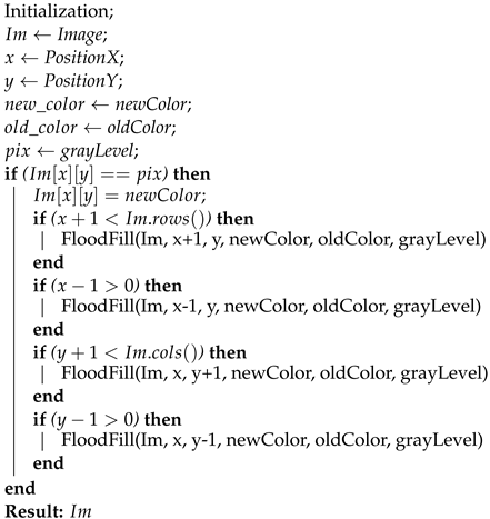 |
Once the image contains the items labeled with a gray level, the process of selecting the best muéganos is performed. Two fundamental conditions are considered for the selection of the muéganos:
- 1.
- Two or more items have contiguous pixels.
- 2.
- There is a limit of contiguous pixels between two items.
Contiguous pixels are adjacent pixels between neighboring item borders. If there are more adjacent pixels between items, there is less wastage.
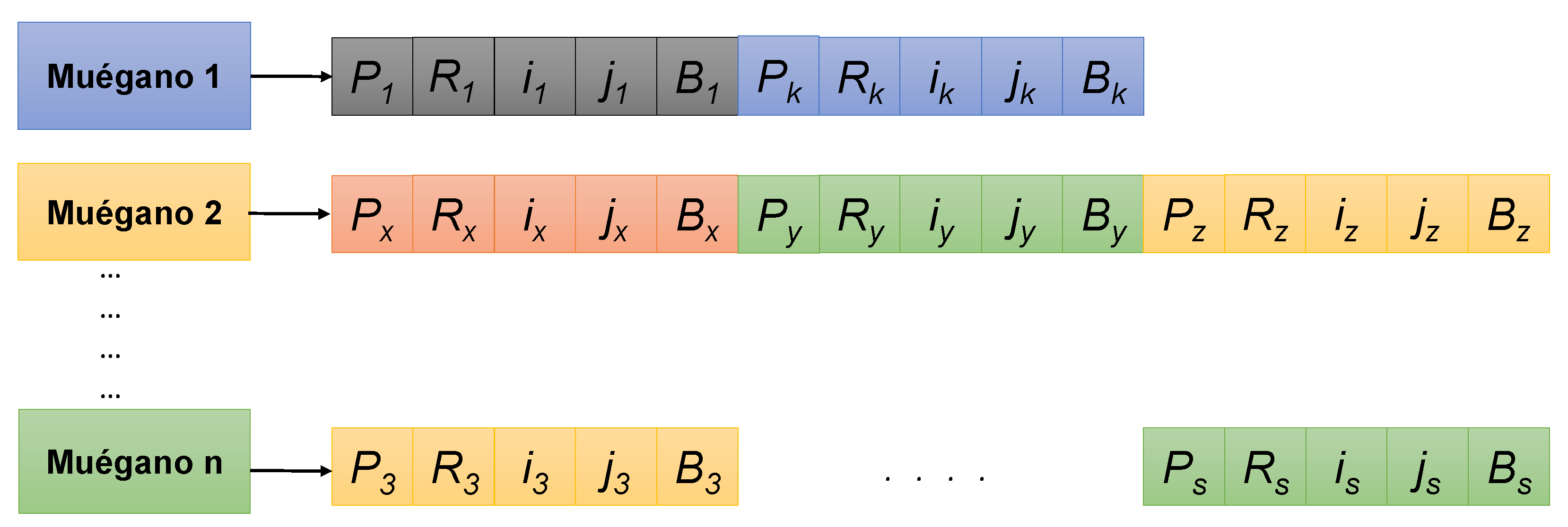
A data structure containing the information of each muégano was implemented, in other words, the number of items contained in each muégano as shown in Figure 6.

Figure 6.
Muégano structure. Each muégano is a list of the contained items. The number of items depends on the largest number of adjacent pixels between edges of neighboring items.
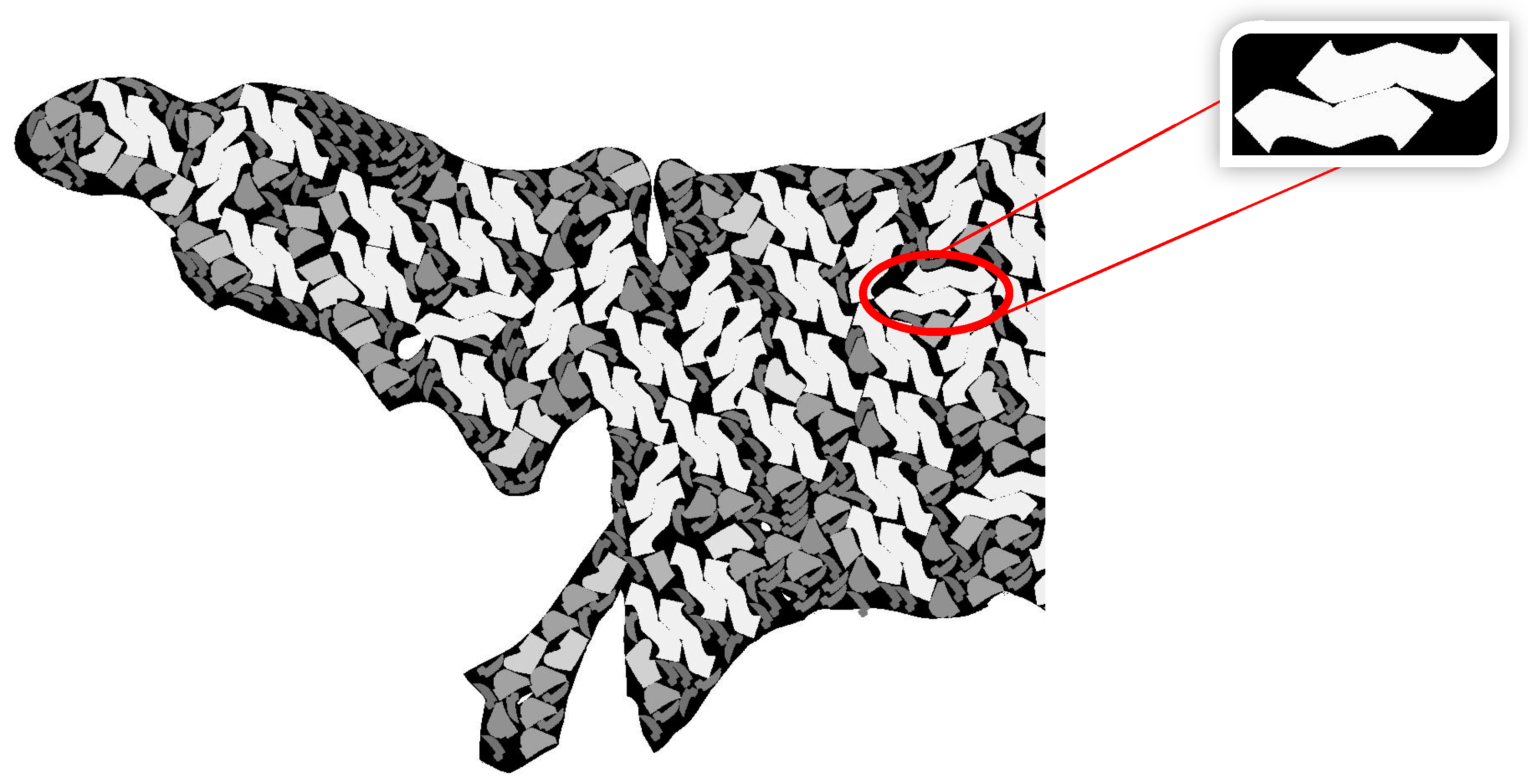
An example of muégano formation is shown in Figure 7.
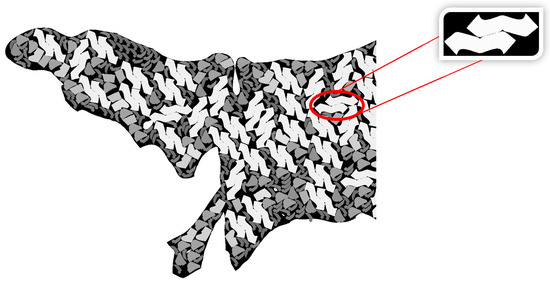
Figure 7.
Sample nesting results. Inside of the red ellipse: example of muégano formed by two items. Each item has a different gray level.
2.6. Sequential Greedy Algorithm
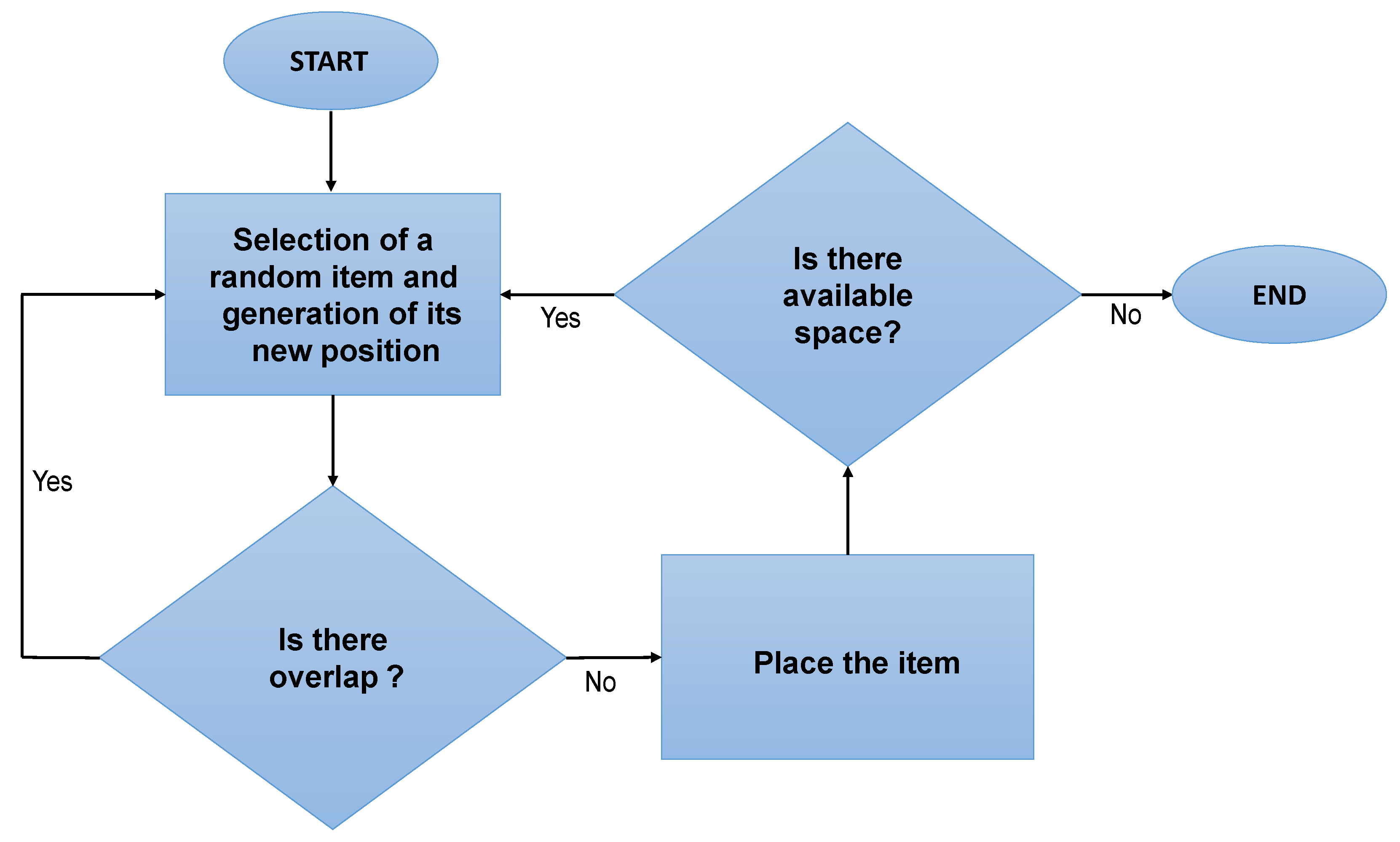
Once the muéganos are generated, a sequential greedy algorithm (SGA) is implemented to fill the area of the material that has not been used. Figure 8 shows the flow diagram of the SGA. Items and muéganos are randomly selected and nested avoiding overlaps between them, until there is no more space in the material.
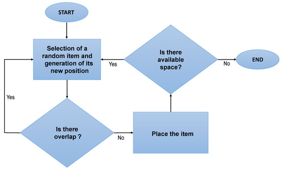
Figure 8.
Flow diagram of the greedy sequential algorithm to fill the area of the unused material. The random item is selected, and its position is generated. If the item is non-overlapped with another one, it is placed. The process is looped while there is available space in the material.
3. Experimental Results
This section shows the results obtained by applying the techniques explained above. The term in Equation (5) was used to obtain the wastage in square meters (m2) of the resulting images. The standard deviation was calculated to measure the precision according to the value obtained for the waste in the same image by repeatedly calculating the term .
In this research, materials obtained from a leather-footwear factory were utilized, including cowhide leather material and boot-type footwear patterns. These materials were processed following the arrangement outlined in the “Calculation of waste in metric values” Section 2.2, to obtain their real and pixel sizes. Subsequently, the procedure described in the “Methodology” Section 2 was employed to generate the results presented in this section.
The results were obtained using 60 muéganos in the solutions. The quantity of muéganos is equivalent to 120 items, which were used to form the solutions in the results obtained without muéganos. Table 4 and Table 5 show the results of twenty runs with and without muéganos, respectively. Each run represents a solution obtained by nesting the items on the material. The columns specify the percentage of wastage and its equivalent in m2, the execution time, and the admissible orientations for each item.
Table 4.
Results obtained without Muéganos.
Table 5.
Results obtained with Muéganos.
Figure 9 represents a comparison for the waste value between the solutions with and without muéganos. It is essential to mention that the worst solution with muéganos achieves a lower wastage than the best solution without them. This proposed method improves the solution and reduces waste.
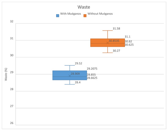
Figure 9.
Comparison of waste between the results obtained with and without muéganos. The blue box-and-whisker plot shows a better improvement of the waste over the non-muéganos box-and-whisker plot. The mean of the results using muéganos is around .
Figure 10 illustrates the execution time, comparing the solutions with and without muéganos. Since they are formed by more compact items, it takes longer to place them in the material as it seeks for a larger area to perform the arrangement. However, this compensates for the fact that the waste is reduced.
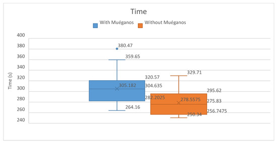
Figure 10.
Comparison of time between the results obtained with and without muéganos. The blue box-and-whisker plot shows a greater spread of computational time cost, and the mean of the results is around 305 s due to the size of the muéganos structure. However, it is compensated by reduced waste.
Figure 11 shows the obtained results without and with muéganos, respectively. Figure 11a shows the items placed randomly, which results in less compactness between them when nesting. The execution time of the solution was 260.68 s. Figure 11b illustrates a higher compaction between two items contained in the muégano, with an execution time of s.
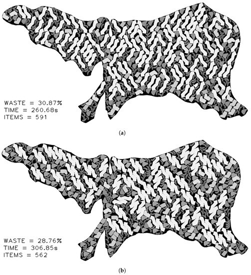
Figure 11.
Nesting results obtained (a) without muéganos, and (b) with muéganos. The result obtained from muéganos and item nesting generates less waste than the non-muéganos solution due to the minimum separation between items inside the muéganos structure.
Comparisons with Other Research
Some comparisons were made with other methods proposed in the literature. In [4], they used a greedy algorithm with a bottom-left strategy to placed the items obtaining an efficiency of . In this work the concept of muéganos was applied to find the solution obtained with an efficiency of as shown in Figure 12a. In [30], a separation and compaction algorithm using a fast obstruction map local search (FOMLS) was developed to solve a rectangular packing problem (RPP) using fixed-ratio compaction. They obtained an efficiency of , which, compared to the result of this research using the muéganos, obtained an improvement with efficiency. Figure 12b shows our result. In [27], calculating with BRKGA70 for the instances with circles obtained an efficiency of . In our case, we performed some runs with the same patterns on a finite material obtaining efficiency, as shown in Figure 12c.
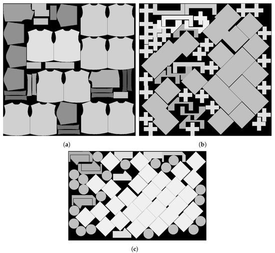
Figure 12.
Results obtained by our method using state-of-the-art patterns. We used (a) the items from [4], (b) from [30], and (c) from [27] to compare the waste and efficiency.
Table 6 displays the comparative results of our work against other methods. The three initial columns present references and values of efficiency and waste obtained from the reported methods. The final two columns exhibit outcomes from the proposed method in this study, derived through item utilization from the compared methods.
Table 6.
Comparative results with the state-of-the-art.
4. Discussion and Future Work
This paper proposes a strategy to repair solutions obtained with overlaps using metaheuristics, which provides an excellent alternative to solve the nesting problem and allows an improved matching process. The muéganos structure aims to compact the items to reduce waste, and this work demonstrates that feasible solutions are obtained to compete with the results achieved in previous research. It is important to mention that the repair process and the muéganos can be applied to any solution to solve the nesting problem, as long as there is an overlap in any solution.
The method proposed in this research is applied to real problems in industries such as the leather-footwear industry, where waste reduction is crucial for optimal material utilization. Many companies still manually conduct nesting processes, relying on operator expertise, impacting time and material waste. Automation of the nesting process is vital for efficiency. Specialized companies have provided us with the required materials (including leather material and footwear patterns) to conduct real-size testing. Additionally, we established an arrangement within the factory to capture images of the materials, facilitating the subsequent calibration and image digitization processes.
The proposed method offers a significant advantage in automating the nesting process within these industries, leading to decreased material waste and increased efficiency. Although this method has advantages over other reported ones, it has certain limitations, but working on these can lead to even better results. For example, time production is a important factor in the industry when working in real-time, and this improvement could make the algorithm more efficient. In future work, the time factor will be improved by using parallel programming with threads in the implementation of the algorithm. Additionally, it is convenient to keep a count of all the items needed to complete the manufacturing process depending on the type of industry in which the algorithm is applied.
To further improve results, it is necessary to work on determining the quality of the skin to give an adequate positioning to each item. The skin segmentation is by type of cut, since each item must have a certain elasticity, and therefore must be placed in a suitable orientation angle. Another future work is to calculate the efficiency of wastage by muéganos to provide solutions with the least possible waste. Finally, a further improvement will be to achieve the formation of muéganos per production unit; for example, if a shoe needs five items for its manufacture, then the muéganos should contain these five items.
Author Contributions
Conceptualization, A.R. and F.C.; methodology, A.R. and F.C.; software, A.R.; validation, A.R. and F.C.; formal analysis, A.R. and F.C.; investigation, A.R.; resources, A.R., F.C. and D.E.; data curation, A.R.; writing—original draft preparation, A.R. and D.E.; writing—review and editing, A.R. and F.C.; visualization, A.R.; supervision, F.C.; project administration, F.C.; funding acquisition, F.C. All authors have read and agreed to the published version of the manuscript.
Funding
This research received no external funding.
Institutional Review Board Statement
Not applicable.
Informed Consent Statement
Not applicable.
Data Availability Statement
Not applicable.
Acknowledgments
The authors wanted to thank Centro de Investigaciones en Óptica A. C. (CIO) and Consejo Nacional de Humanidades Ciencia y Tecnología (CONAHCYT) for giving us the opportunity to develop this research. We would like to thank the following shoe factories Tecnoboots and Lobosolo for providing us the necessary materials for the tests. We would like to express our gratitude for the collaboration of the English teachers Mario Alberto Ruiz Berganza and Karla Maria Ivonne Noriega Cos, for their valuable contributions in revising the language.
Conflicts of Interest
The authors declare no conflict of interest.
Abbreviations
The following abbreviations are used in this manuscript:
| GAs | genetic algorithms |
| SA | simulated annealing |
| ANNs | artificial neural networks |
| PSO | particle swarm optimization |
| SGA | sequential greedy algorithm |
| QHDP | quick heuristic dynamic programming |
| NFP | no-fit polygon |
| RKGA | random-key genetic algorithm |
| BRKGA | biased random-key genetic algorithm |
| MIP | mixed-integer programming |
| FOMLS | fast obstruction map local search |
| RPP | rectangular packing problem |
References
- Gonzalez, R.C.; Woods, R.E. Digital Image Processing, 3rd ed.; Pearson Education, Inc.: Upper Saddle River, NJ, USA, 2008. [Google Scholar]
- Martí, R. Multi-Start Methods. In Handbook of Metaheuristics; Glover, F., Kochenberger, G.A., Eds.; Springer: Boston, MA, USA, 2003; pp. 355–368. [Google Scholar] [CrossRef]
- Reeves, C.R. Modern Heuristic Techniques for Combinatorial Problems; John Wiley & Sons, Inc.: New York, NY, USA, 1993; Chapter Genetic Algorithms; pp. 151–196. [Google Scholar]
- Fischetti, M.; Luzzi, I. Mixed-integer programming models for nesting problems. J. Heuristics 2009, 15, 201–226. [Google Scholar] [CrossRef]
- Leung, S.C.; Zhang, D.; Zhou, C.; Wu, T. A hybrid simulated annealing metaheuristic algorithm for the two-dimensional knapsack packing problem. Comput. Oper. Res. 2012, 39, 64–73. [Google Scholar] [CrossRef]
- Wei, L.; Hu, Q.; Lim, A.; Liu, Q. A best-fit branch-and-bound heuristic for the unconstrained two-dimensional non-guillotine cutting problem. Eur. J. Oper. Res. 2018, 270, 448–474. [Google Scholar] [CrossRef]
- Kirkpatrick, S.; Gelatt, C.D.; Vecchi, M.P. Optimization by simulated annealing. Science 1983, 220, 671–680. [Google Scholar] [CrossRef]
- Poli, R.; Kennedy, J.; Blackwell, T. Particle swarm optimization. Swarm Intell. 2007, 1, 33–57. [Google Scholar] [CrossRef]
- Eberhart, R.; Kennedy, J. A new optimizer using particle swarm theory. In Proceedings of the MHS’95, Sixth International Symposium on Micro Machine and Human Science, Nagoya, Japan, 4–6 October 1995; pp. 39–43. [Google Scholar] [CrossRef]
- Goldberg, D.E. Genetic Algorithms in Search, Optimization and Machine Learning, 1st ed.; Addison-Wesley Longman Publishing Co., Inc.: Boston, MA, USA, 1989. [Google Scholar]
- Leakey, R.E. Charles Darwing, El Origen de Las Especies. Versión Abreviada, 1st ed.; Martín Casillas Editores, S. A.: Mexico, 1980. [Google Scholar]
- Cuevas, F.; Gonzalez, O.; Susuki, Y.; Hernandez, D.; Rocha, M.; Alcala, N. Genetic algorithms applied to optics and engineering. In Proceedings of the Fifth Symposium Optics in Industry, Santiago De Queretaro, Mexico, 8–9 September 2006; Rosas, E., Cardoso, R., Bermudez, J.C., Barbosa-GarcÃa, O., Eds.; International Society for Optics and Photonics, SPIE: Bellingham, DC, USA, 2006; Volume 6046, pp. 360–368. [Google Scholar] [CrossRef]
- Holland, J. Adaptation in Natural and Artificial Systems: An Introductory Analysis with Applications to Biology, Control, and Artificial Intelligence; University of Michigan Press: Ann Arbor, MI, USA, 1975. [Google Scholar]
- Talbi, E. Metaheuristics: From Design to Implementation; Wiley Series on Parallel and Distributed Computing; Wiley: Hoboken, NJ, USA, 2009. [Google Scholar]
- Gen, M.; Cheng, R.; Lin, L. Network Models and Optimization: Multiobjective Genetic Algorithm Approach; Springer: Berlin/Heidelberg, Germany, 2008. [Google Scholar]
- Cui, Y.P.; Cui, Y.; Tang, T. Sequential heuristic for the two-dimensional bin-packing problem. Eur. J. Oper. Res. 2015, 240, 43–53. [Google Scholar] [CrossRef]
- Zhang, D.; Shi, L.; Leung, S.; Wu, T. A priority heuristic for the guillotine rectangular packing problem. Inf. Process. Lett. 2016, 116, 15–21. [Google Scholar] [CrossRef]
- Gomez, J.C.; Terashima-Marín, H. Evolutionary hyper-heuristics for tackling bi-objective 2D bin packing problems. Genet. Program. Evolvable Mach. 2017, 19, 151–181. [Google Scholar] [CrossRef]
- Leung, S.C.; Zhang, D.; Sim, K.M. A two-stage intelligent search algorithm for the two-dimensional strip packing problem. Eur. J. Oper. Res. 2011, 215, 57–69. [Google Scholar] [CrossRef]
- Júnior, A.N.; Silva, E.; Gomes, A.M.; Soares, C.; Oliveira, J. Data mining based framework to assess solution quality for the rectangular 2D Strip-Packing Problem. Expert Syst. Appl. 2018, 118, 365–380. [Google Scholar] [CrossRef]
- Yin, A.; Huang, J.; Hu, D.; Chen, C. A Quick Heuristic-Dynamic Programming for Two-Dimensional Cutting Problem. In Proceedings of the 2019 IEEE 5th International Conference on Computer and Communications (ICCC), Chengdu, China, 6–9 December 2019; pp. 164–169. [Google Scholar]
- Pinheiro, P.R.; Júnior, B.A.; Saraiva, R.D. A random-key genetic algorithm for solving the nesting problem. Int. J. Comput. Integr. Manuf. 2016, 29, 1159–1165. [Google Scholar] [CrossRef]
- Rashid, D.N.H.; Rashid, T.A.; Mirjalili, S. ANA: Ant Nesting Algorithm for Optimizing Real-World Problems. CoRR 2021, abs/2112.05839. Available online: http://xxx.lanl.gov/abs/2112.05839 (accessed on 2 December 2021).
- Ding, B.; Zhang, R.; Xu, L.; Liu, G.; Yang, S.; Liu, Y.; Zhang, Q. U2D2Net: Unsupervised Unified Image Dehazing and Denoising Network for Single Hazy Image Enhancement. IEEE Trans. Multimed. 2023, 1–16. [Google Scholar] [CrossRef]
- Zhang, R.; Yang, S.; Zhang, Q.; Xu, L.; He, Y.; Zhang, F. Graph-based few-shot learning with transformed feature propagation and optimal class allocation. Neurocomputing 2022, 470, 247–256. [Google Scholar] [CrossRef]
- Poshyanonda, P.; Dagli, C.H. Genetic neuro-nester. J. Intell. Manuf. 2004, 15, 201–218. [Google Scholar] [CrossRef]
- Mundim, L.R.; Andretta, M.; de Queiroz, T.A. A biased random key genetic algorithm for open dimension nesting problems using no-fit raster. Expert Syst. Appl. 2017, 81, 358–371. [Google Scholar] [CrossRef]
- Kierkosz, I.; Luczak, M. A one-pass heuristic for nesting problems. Oper. Res. Decis. 2019, 1, 37–60. [Google Scholar]
- Bennell, J.A.; Song, X. A comprehensive and robust procedure for obtaining the nofit polygon using Minkowski sums. Comput. Oper. Res. 2008, 35, 267–281. [Google Scholar] [CrossRef]
- Sato, A.K.; Mundim, L.R.; Martins, T.C.; Tsuzuki, M.S.G. A separation and compaction algorithm for the two-open dimension nesting problem using penetration-fit raster and obstruction map. Expert Syst. Appl. 2023, 220, 119716. [Google Scholar] [CrossRef]
- Bäck, T.; Fogel, D.B.; Michalewicz, Z. Evolutionary Computation 2: Advanced Algorithms and Operators; CRC Press: Boca Raton, FL, USA, 2000. [Google Scholar]
- Whitley, L.D.; Gordon, V.S.; Mathias, K.E. Lamarckian Evolution, The Baldwin Effect and Function Optimization. In Proceedings of the International Conference on Evolutionary Computation, the Third Conference on Parallel Problem Solving from Nature—PPSN III: Parallel Problem Solving from Nature, Jerusalem, Israel, 9–14 October 1994; Springer: Berlin/Heidelberg, Germany, 1994; pp. 6–15. [Google Scholar]
- Otsu, N. A Threshold Selection Method from Gray-Level Histograms. IEEE Trans. Syst. Man Cybern. 1979, 9, 62–66. [Google Scholar] [CrossRef]
- Astrachan, O.L. Bubble sort: An archaeological algorithmic analysis. In Proceedings of the Technical Symposium on Computer Science Education, Reno, NV, USA, 19–23 February 2003. [Google Scholar]
- Zhang, Z. A flexible new technique for camera calibration. IEEE Trans. Pattern Anal. Mach. Intell. 2000, 22, 1330–1334. [Google Scholar] [CrossRef]
- Hartley, R.I.; Zisserman, A. Multiple View Geometry in Computer Vision, 2nd ed.; Cambridge University Press: Cambridge, UK, 2004; ISBN 0521540518. [Google Scholar]


Disclaimer/Publisher’s Note: The statements, opinions and data contained in all publications are solely those of the individual author(s) and contributor(s) and not of MDPI and/or the editor(s). MDPI and/or the editor(s) disclaim responsibility for any injury to people or property resulting from any ideas, methods, instructions or products referred to in the content. |
© 2023 by the authors. Licensee MDPI, Basel, Switzerland. This article is an open access article distributed under the terms and conditions of the Creative Commons Attribution (CC BY) license (https://creativecommons.org/licenses/by/4.0/).