Abstract
Exact and complete preparation of a hydrographic survey project allows for the avoidance or reduction of additional costs and unexpected delays and, at the same time, increases the efficiency of the survey. One of the essential requirements at the survey planning stage is a calculation of time necessary for performing bathymetric measurements with a multi-beam echosounder. Based on these calculations, many decisions related to the costs and methodology are made. The article presents the method of time estimation for the hydrographic surveys and takes into account many variables that directly affect the final duration of the project. The paper demonstrates the influence of water depth, multi-beam echosounder swath angle, and other planning parameters related to the scheme of survey lines on the total time of stay at sea. The main findings are based on the author’s over twenty years of experience aboard the Polish Navy hydrographic ship Arctowski and include thorough analysis of specialist literature, publications, manuals, and international standards.
1. Introduction
At the beginning of their adventures at sea, people only went out during the day for safety reasons. With the invention of the compass, sailors began to use the stars and draw maps. The growing demands of sailors, travelers, and researchers were the impetus for developing depth measurement methods and techniques that have evolved over the centuries from very simple techniques to the complex and technologically advanced.
For hundreds of years, the only possible way to measure the depth of seas and oceans was a calibrated hemp rope terminating in a weight lowered from the side of the vessel. Until World War II, most depth measurements were made with the use of a lead line. That method was not only inaccurate but also very time-consuming. World War I and II saw the rapid development of echosounders and simple sonar. Since then, the need for updated nautical charts has increased. This was dictated by the increase in traffic in the coastal zone, the growing popularity of recreational shipping, and the continually developing world maritime trade. The necessity to update the charts forced the state hydrographic services to conduct systematic marine surveys using single-beam echosounders (SBESs) within territorial waters. Hydrographic vertical echosounders became increasingly available, which positively impacted the safety of navigation and the accuracy of nautical charts [1,2].
Scientists were interested not only in the depths directly under the ship’s hull but also those at some lateral distance from it. New military and defense challenges and cognitive needs have prompted scientists and engineers to start work on new technological solutions in sea bottom research. These efforts led to the development of a new technology, multi-beam echosounders (MBESs), which were initially a secret project of the US Navy in the 1950s [3,4,5].
The last three decades have seen a dynamic advancement in survey technologies. Multi-beam echosounders providing full seabed coverage have become very popular. Their attractiveness is associated with an increased quality and quantity of data as well as much greater coverage. Measurements obtained via this method are used in many scientific fields, including seabed imaging and classification [6,7,8,9,10], learning about the processes occurring in bottom sediments [11,12,13], identifying geotechnical hazards and gas leakages from the seabed [14], and exploration of the marine habitat [15,16,17,18]. MBES is widely used in the operations of laying of trans-oceanic telephone cables, exploration and drilling for the oil extraction industry, locating underwater mineral deposits, and learning about Earths geological processes [19,20,21,22]. These swath systems are also successfully used in the study of underwater cultural heritage [23,24].
The primary and most common application of modern multi-beam echosounders is the multi-point and multi-directional measurement of depth values for the purpose of navigation safety and marine cartography [25,26]. The ability to record the depth simultaneously via several hundred points on the sea bottom together with their associated positions is undoubtedly an advantage of this device, which has been noticed by scientists of various specialties [27,28,29,30,31,32]. The authors emphasize not only the wide coverage of MBES bathymetric measurements but also the susceptibility of the external beams of the multi-beam systems to various factors that reduce depth measurement accuracy.
Hydrographic surveys executed with the use of MBES are carried out, among others, to ensure safety of navigation through developing nautical charts and marine publications and updating digital databases of underwater objects [33]. Each survey requires detailed planning and thorough preparation, especially since the costs, due to the equipment used, are incomparably higher than for land measurements [34,35]. Accurate and comprehensive preparation of survey projects allows for avoidance or minimization of additional costs and unexpected delays and, at the same time, increases the efficiency of the survey. Planning hydrographic works covers many issues related to the location of measurement reservoirs, the availability of survey platforms, the efficiency of hydrographic equipment, the analysis of qualified hydrographic staff resources, and many other undertakings [36]. It is necessary to check the survey equipment in terms of technical capabilities and availability. In some cases, it may be necessary to carry out a reconnaissance of the research area, check the availability of mareographs, and analyze the traffic intensity. One of the essential requirements of the survey planning stage is a time calculation. Based on these calculations, many decisions related to the costs and methodology are made [37].
To date, no methods and procedures are available with which to calculate the total time needed to perform a systematic bathymetric survey with MBES. The time is estimated based on the number of MBES swaths that should be covered and the subjective opinions and experience of the hydrographers and multi-beam echosounder users. Planning a Naval or civilian hydrographic ship’s stay at sea requires its commander or captain to precisely specify the date and time of departure and return to the harbor. In the public sector, calculating the total time of a field operation is an integral part of costs estimation. In this manuscript, a proprietary method for calculating the time of survey works using a multi-beam echosounder has been proposed. Planning a hydrographic survey involves many decisions and selections. The method of bathymetric measurements with MBES presented in this article will be useful for hydrographic surveyors, planners, scientists, and MBES users. This method will be beneficial for budgeting and the effective use of available personnel, survey equipment, and vessels.
Due to the extensive ocean area and restricted human and material resources, hydrographic surveys should be conducted in a careful and well-planned way. Therefore, the scientific planning of the hydrographic works to ensure the survey effectiveness has become a crucial problem to be addressed by the hydrographic office of each sea state.
2. Materials and Methods
Planning a survey vessel stay at sea requires the captain to precisely plan the date and time of departure and return to the homeport. In the case of hydrographic ships, it is crucial to calculate the total time needed to perform a marine survey. The time depends on the size and depths of the water bodies, the survey speed, and the number of survey track lines. Ensuring the proper organization of the work and the optimal use of the multi-beam system becomes fundamental when it is necessary to meet the requirements of full bottom coverage. Optimal survey planning requires the provision of information about the swath width for a given depth. The Technical Project and the Technical Task for hydrographic survey do not specify the survey parameters in detail. These documents only indicate by which criteria the survey should be carried out. The choice of the swath width is at the hydrographer’s discretion.
Planning hydrographic works is, among other things, the process of determining the optimal parameters of the survey that affect the fulfillment of the requirements specified in the contract, project, or technical task [3]. An inseparable element is studying existing charts, archival sources of information about the bottom shape, the depth distribution, or the presence of navigational hazards. Such data can be used to determine initial survey parameters such as the distance between the survey lines, the bottom coverage, the size of the overlap, or the number of cross lines.
2.1. Model of Estimating the Time of MBES Bathymetric Survey
The distance between the main lines or check lines (crosslines) and their general distribution will largely depend on the size and location of the test water reservoir and the requirements included in the specification. The initial layout of the survey lines and orientation should be prepared in the initial planning stage. That system may be subject to modifications resulting from a better adaptation to the site bottom shape, the layout of the contours, the weather conditions, the intensity of vessel traffic, the occurrence of panicles, and other environmental factors. In measurements with a single-beam echosounder, the sounding lines are designed perpendicular to the general course of the contours. In the case of multi-beam sonar, the main survey lines should follow the direction of the isobaths. The parallel arrangement of the survey lines in relation to the local isobaths ensures, as far as possible, uniform bottom coverage and the maximum use of the optimal swath angle of the multi-beam echosounder.
The calculation of the time necessary to perform the survey should include many variables. The most important are the time needed to perform depth measurements on the main survey lines, the calibration of MBES (patch test), the reach of the survey site, the return to the port, and the time that should be allocated to verify discovered underwater objects and potential delays or interruptions in the survey process resulting from various external factors. The total time of survey measurements is calculated from:
where the following definitions apply:
- total time of the depth measurements on main survey lines [h];
- total time of the depth measurements on cross check lines [h];
- time to perform MBES calibration (patch test) [h];
- total time of cross-check maneuvers [h];
- time of transit to survey site and return to the port [h];
- delay time due to weather conditions [h];
- delay in the survey due to equipment failure [h];
- time spent on examination of detected underwater objects [h].
2.2. Determination of Survey Line Specing
One of the most critical requirements for hydrographic survey work using a multi-beam echosounder is that we ensure full bottom bathymetric coverage. To meet the above condition, the hydrographer is obliged to determine, calculate, or accept, based on expert knowledge and experience, the distance between survey profiles the (line spacing). Based on the average depth of survey area and the swath angle of the multi-beam echosounder, the distance between the survey lines can be determined from the formula:
where average depth of the survey area [m]; swath angle of the multi-beam echosounder [°].
However, Formula (2) does not take into account the possibility of the vessel deviating from the track line and the potential measurement errors on the edge of the MBES swath width. The resulting gaps in data recording can always be covered by performing additional, complementary transitions along the lines, which comes with extra time.
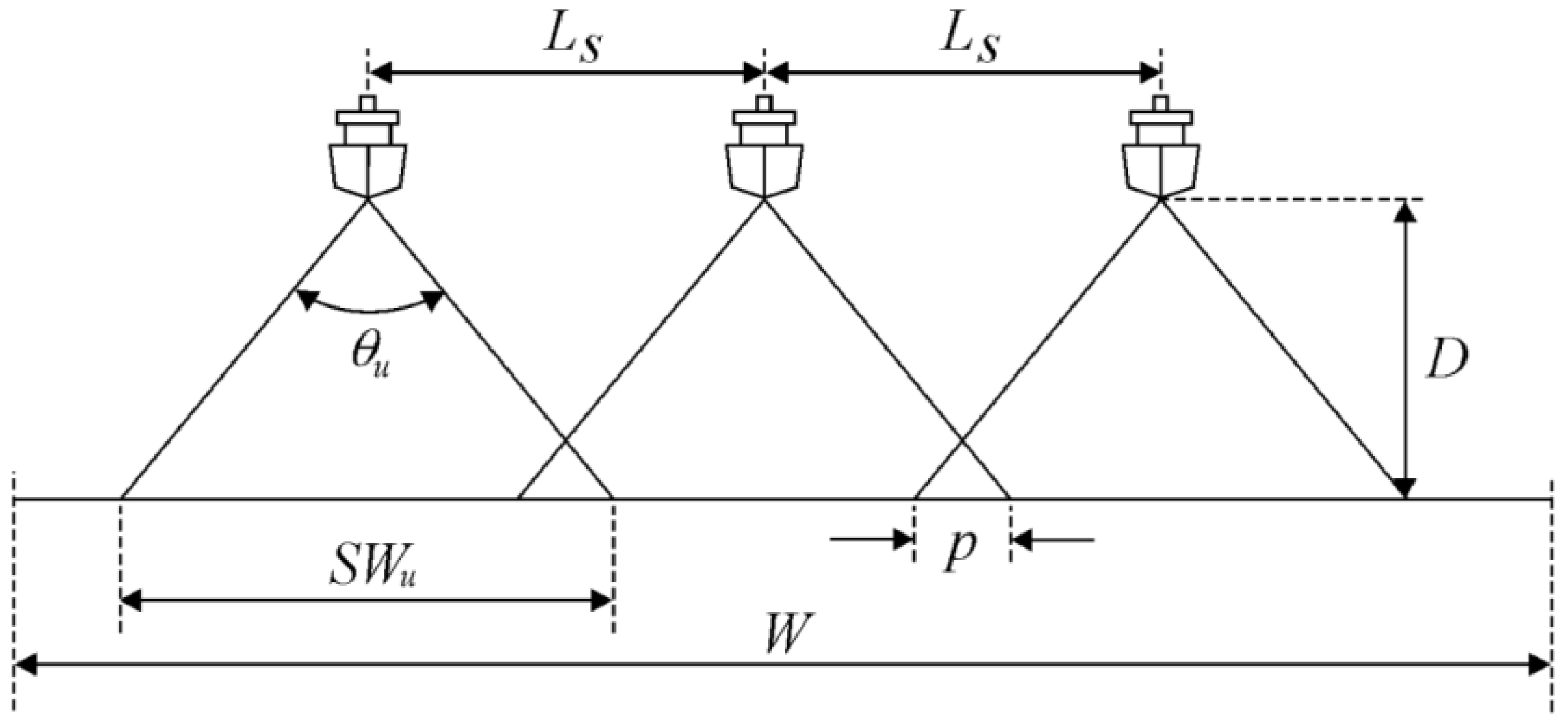
The distance between the survey lines should consider the zone of double depth measurements between two adjacent lines. This zone is called “overlap” and the bottom coverage in this area equals 200% (Figure 1). Overlap is crucial as it allows for the maintenance of depth measurement continuity in cases where the helmsman cannot keep the track line. This zone can also be used as a data quality control measure. The size of overlap mostly depends on the MBES operator’s experience, the specification of the contract requirements, or the order of hydrographic survey work.

Figure 1.
Survey planning parameters using multi-beam echosounder (p—overlap; —useful swath width of MBES; W—width of the survey area; D—average depth of the survey area).
Based on Figure 1,
where —distance between the survey lines [m]; —useful swath width of the MBES [m]; and —overlap [m].
Simplifying the dependence (3), we obtain
Since
where is the useful swath angle of the multi-beam echosounder [°], and assuming that the overlap p is a percentage of the entire swath width, the distance between the survey lines (line spacing) is calculated from the following relationship:
where is the overlap, being a percentage of the useful swath width of the MBES, taking values from 10 to 25%.
Finally,
2.3. Estimation of Measurment Time Spent on Survey Lines
Knowing the parameter of the distance between the survey lines and the width of the survey area, the number of main survey lines is determined as follows:
where W—width of the survey area [m].
The next step is to calculate the total length of the main survey lines . Assuming that the average length of the main survey line is equal to the length of the research area, the total length of the main survey lines is calculated from the product:
where —length of a single main survey line [m].
Assuming that the length of a single cross lines is approximately equal to the width of the survey area W, the total length of the cross lines is obtained from the following relationship:
where —number of planned cross lines; —length of a single cross line [m].
Cross lines are used to assess the accuracy of measurements performed on the main scheme survey lines. They enable the detection of random and systematic errors. In good weather conditions, the direction of the cross lines should be perpendicular to the direction of the main lines and the measurements conducted at the beginning of the survey [35,38,39]. These measurements additionally increase the survey data density. The guidelines of the International Shipowners Association IMCA [3] recommend that when surveying with a multi-beam echosounder, depth measurements should be made on at least two cross lines. The more varied and irregular the bottom surface is, the greater the number of cross lines required. For large water bodies (e.g., 10 km by 30 km), the cross lines should be designed every 1–5 km. The Canadian standards for hydrographic measurements state that the distance between the cross lines should not be greater than fifteen times the distance between the basic profiles [40]. Ultimately, the number of cross lines will depend on the size of the survey water body, the shape of the bottom, and the requirements contained in the specification. The final decision is made by the hydrographer responsible for the entire survey project. The layout of the main and cross lines schemes and the basic survey parameters are presented in Figure 2.
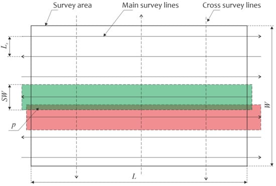
Figure 2.
Layout of the main and cross survey lines.
The decision regarding the line orientation and spacing for the methodical sounding of an area will be influenced by the equipment to be used. The total time spent conducting depth measurements following the main survey lines includes the time spent measuring the main tracks, the time necessary for vessel turns, and the time spent measuring the speed of sound in water column:
where —survey time on main lines [s]; —time necessary to perform vessel turns [s]; and —time for measuring speed of sound in the water column [s]. Formula (11) is developed to the following form:
where —vessel speed on the main survey lines [m/s]; —time to perform vessel turn to the next main lines [s]; —number of SVP measurements; and —time of a single measurement of SVP [s].
The time of survey measurements on cross lines is derived from:
where —time of bathymetric measurement on cross lines [s]; —time necessary to perform vessel turns [s].
The distance between the cross lines is usually much greater than the distance between the main line; thus, the survey vessel will probably move at maximum speed to the next cross line. Given the number of cross lines and the speed of the platform while maneuvering to the next line, the total duration of turns on the cross lines is calculated using the following formula:
where —vessel speed at turns to the next cross line [m/s].
Thus, the total time needed to perform the control measurements can be simplified to the equation:
where —total time of bathymetric measurements on cross lines [s]; —platform speed on cross lines [m/s].
2.4. Other Factors Affecting the Total MBES Survey Time
In addition to the time necessary to perform measurements on the survey lines, the following three parameters should also be included in the time calculations:
- Time to perform patch test calibration—;
- Total time devoted to cross-check maneuvers;
- Time to reach the research area and return to the port—.
Before the start of the survey, the hydrographer should perform the calibration of the multi-beam echosounder called patch test. The test enables the determination of errors in measuring the mounting angles of the MBES sonar head. As a result, corrections are obtained for which the initial angular values of the transducer should be corrected. Calibration should be performed, if possible, in good weather conditions, and in an area with a depth and bottom type similar to the planned survey area [39].
A cross-check maneuver is performed, especially in the outermost beam sectors, to check the correctness of the sonar operation and measurement accuracy [41]. The multi-beam echosounder performance should be checked each time before and after the hydrographic works, but also during the survey if the hydrographer deems such action necessary and justified. The cross-check maneuver consists of making two passes on profiles perpendicular to each other and then comparing the readings of outer acoustic beams with the readings of vertical beams. The total time allocated to cross-check maneuvers is calculated according as follows:
where —number of cross-check maneuvers; —time of a single cross-check maneuver [s].
The time of reaching the survey area and returning to the home port is calculated according to the following:
where —distance to the area of hydrographic works [m]; —vessel’s speed at the transition to the survey area and return to the port [m/s].
The time spent on calibration, control maneuvers, and transition to the survey area are forecast variables given as an approximation. These parameters may change after, e.g., deterioration of weather conditions, resignation, extension of the patch test time, or an increase in the number of cross-check maneuvers.
It is extremely important that the survey plan is flexible, that is, that it considers possible delays caused by changing weather conditions, survey equipment malfunctions, or failures of main power plant of the vessel, which cannot be predicted or avoided. Hence, the total time required to perform a specific hydrographic survey should also take into account the so-called survey delay time:
where —time of the survey interruption due to weather conditions [s]; —time of the survey interruption due to equipment failure [s].
In the event of detection of underwater objects (i.e., navigational obstructions) lying in the area of the survey works, additional hydrographic research should be performed to obtain as much information about the target as possible. It often happens that the object is a new object that has not appeared in the available digital databases and has not been plotted on the charts. As part of additional activities at sea, bathymetric and sonar measurements are carried out to assess the type and size of the object and the degree of risk to navigation. Such bathymetric and sonar verification is associated with additional time to be predicted in the time calculation. The time is calculated based on the following formula:
where —time of bathymetric measurements in the area of the newly detected underwater object [s]; —time of sonar survey in the area of the newly detected underwater object [s]; and —number of detected underwater objects.
2.5. The Total Time of Hydrographic Survey Conducted with MBES
The calculated time of survey execution is a variable that depends on many factors that cannot be fully predicted. Therefore, time estimation is not an easy task. External factors may extend the total survey time by 5–20% [28]. If the survey work is carried out for the first time in a given basin and there is little information on the bottom shape and depth changes, it may turn out that due to the occurrence of shallows, it is justified to increase the number of survey lines. Such a decision will certainly extend the duration of the survey. Other factors influencing the extension of the time of stay at sea include deviation from the survey line as a result of the excessive approach of another vessel or the setting out of fishing nets by fishermen. The resulting gaps in the data must be covered by re-survey operation. Lack of access to RTK corrections and significant deterioration of position accuracy will make it necessary to repeat measurements on a given survey line. The survey duration may also be extended if it is necessary to perform additional tests, such as quality assurance performance test on multi-beam data. The purpose of this test is to obtain an estimate of the accuracy and, most significantly, of the repeatability of a multi-beam echosounder dataset. The algorithm for determining the hydrographic survey time seems to be one of the essential procedures used by the project manager (the hydrographic division commander onboard navy ship) responsible for a given project.
Given all the dependencies (1)–(19), the total time necessary to perform the hydrographic survey using a multi-beam echosounder is calculated as follows:
The time calculations proposed in this chapter can be an invaluable help in estimating the costs of measurement works, are indispensable in planning ships and hydrographic cutters out to sea, and can be successfully applied to the development of Designs and Technical Tasks by the Polish Naval Hydrographic Office and the Naval Hydrographic Security Division.
3. Results and Discussion
3.1. Duration of Hydrographic Surveys of the Same Water Area for Different Vessel Speeds and MBES Swath Angles
In the first scenario, it was assumed that the same 10 m of depth water area is being considered, and the vessel conducts a bathymetric survey taking into account various MBES swath angles and variable speeds of movement. In order to perform the calculations, the specific parameters presented in Table 1 were adopted.

Table 1.
Hydrographic survey parameters used for calculations in scenario 1.
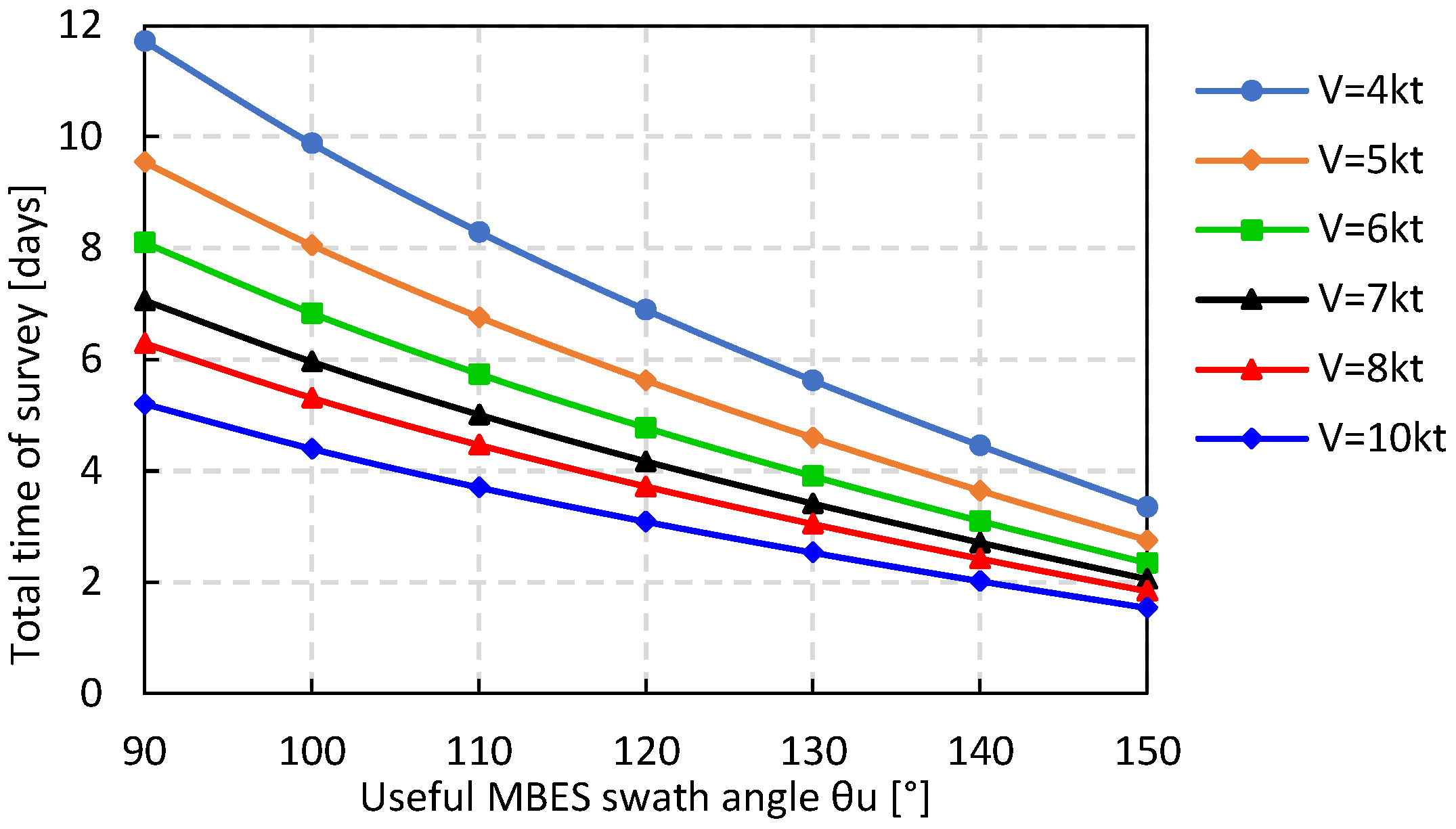
In very shallow water, various opening angles of MBES can be used, most often within the range 90–150°. With the increase in the MBES beamwidth θ, the time of surveying a water area of 5 × 2 Nm with a water depth of 10 m decreases and ranges from almost 12 days for small angles and low speeds (for θu = 90° and Vpp = 4 kt) to almost 1.5 days using the full capabilities of both the survey system and the vessel (for θu = 150° and Vpp = 10 kts). The results of the simulation of the survey duration for the assumed operating parameters are presented in Figure 3.
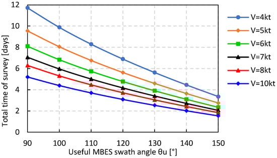
Figure 3.
Estimated time of survey conducted with a multi-beam echosounder as a function of vessel speed and MBES swath angle (water basin 5 × 2 Nm).
Based on the graphs (Figure 3), the selection of the appropriate swath angle of the multi-beam echosounder and the survey speed determine the time necessary to perform the hydrographic survey. For economic reason hydrographer should use the maximum MBES swath angle of 150° and vessel speed of 10 kts. Unfortunately, in practice, there are situations in which contractors, for economic reasons, use the maximum angle of the MBES, thus shortening the time spent in the survey area. The approach of such hydrographers approach may lead to registering the depths with errors, which might be unacceptable to the National Hydrographic Office or the customer.
It is also worth adding that by increasing the swath angle of MBES, the footprint size of the outer beams increases. Thus, the spatial resolution of the echosounder decreases, which directly affects the depth measurement accuracy and detection capabilities of the system. The footprint magnitude near normal incidence (under the transducer) is relatively small; thus, the resolution is higher than for the outer beams. The hydrographer should be aware of how the resolution of the echosounder used changes as a function of the beam pointing angle. Knowing the requirements of the hydrographic survey project, it is possible to select the appropriate size of the MBES swath angle, keeping in mind the resolution parameter. The size of the acoustic footprints of individual MBES beams in the along-track direction, for a flat seafloor, is approximately given by the following:
where ax—the width of the footprint in the fore–aft direction; D—the mean depth [m]; —the beam pointing angle [°]; and —the along-track beamwidth of the MBES [°].
The length of the MBES footprints in the across-track direction is approximately given by the following:
where ay—the width of the footprint in the across-track direction; —the across-track beamwidth of the MBES [°]. The variable MBES resolution values as a function of the beam pointing angles (deviated from Nadir) are presented in Table 2.
Table 2.
The sizes of the footprints of the MBES beams in the along-track and across-track direction. Calculation for a depth of 30 m, = 1°, = 1°.
Many studies have been carried out on the performance of multi-beam echosounders available on the market in recent years. Their results and conclusions have been published, inter alia, in [42,43,44,45,46,47,48]. The publications contain test results for multi-beam echosounders in terms of accuracy requirements and MBES detection capabilities. Many publications are devoted to the depth measurement uncertainty and the error sources that accompany all multi-beam systems. These phenomena have been widely described in [49,50,51,52,53]. Some sources [54,55,56] focus on the analysis of the accuracy and detection capabilities of the external beams of the multi-beam echosounder.
On the basis of research conducted by Grządziel [57] in a basin with a depth of 8–10 m, the useful angular sector of MBES is 140° (maximum θ = 160°). It remains a matter of choosing the appropriate survey speed so that the bathymetric data obtained in this way ensure full bottom coverage, are error-free, and enable the detection of underwater objects. The speed can neither be arbitrary nor the maximum one. Full bathymetric coverage is a criterion required by the IHO standard S-44 [58]. In the case of a multi-beam echosounder, it is vital to achieve full coverage in the direction of the vessel’s movement (the so-called along-track coverage).
Hence, it is very important to determine the maximum vessel’s survey speed that will meet the condition of full coverage in the along-track direction. The maximum speed, Vmax, of the vessel surveying with a multi-beam echosounder under the condition of full coverage is calculated according to [50,57] the following:
where —along-track beamwidth of the MBES [; —speed of sound in the water column [m/s]; and —maximum swath angle of the MBES [°].
The latest models of multi-beam echosounders have very narrow along-track beamwidths. Norbit Winghead i80S has along-track beamwidth of ψx = 0.5°. Teledyne Marine SeaBat T-51-R is characterized by a beamwidth of ψx = 1°, and for the frequency of 700–800 kHz, the beam is even narrower and amounts to ψx = 0.5°. Sonic 2026 produced by R2Sonic, on the other hand, declares the narrowest acoustic beamwidth of ψx = 0.45°. Such narrow beams mean that in order to maintain full bottom coverage and detect underwater objects on the bottom, the maximum surveyed speed should not be exceeded. For a basin with a depth of 10 m, the MBES swath angle θmax = 140° and the along-track beamwidth ψx = 0.5°, the hydrographer should conduct the survey at a speed of Vmax = 4.3 kts. This means that it will take on average 4 days and 4 h.
3.2. Hydrographic Surveys of the Water Body of the Same Area and Different Depths
In the next scenario, it was assumed that the measurements are made in water bodies of different depths but the size of the water area is constant. Simulations were carried out for five different depths of 10 m, 30 m, 50 m, 75 m, and 100 m. In order to perform calculations, specific parameters presented in Table 3 were adopted.
Table 3.
Hydrographic survey parameters used for calculations in scenario 2 (area 6 × 3 Nm).
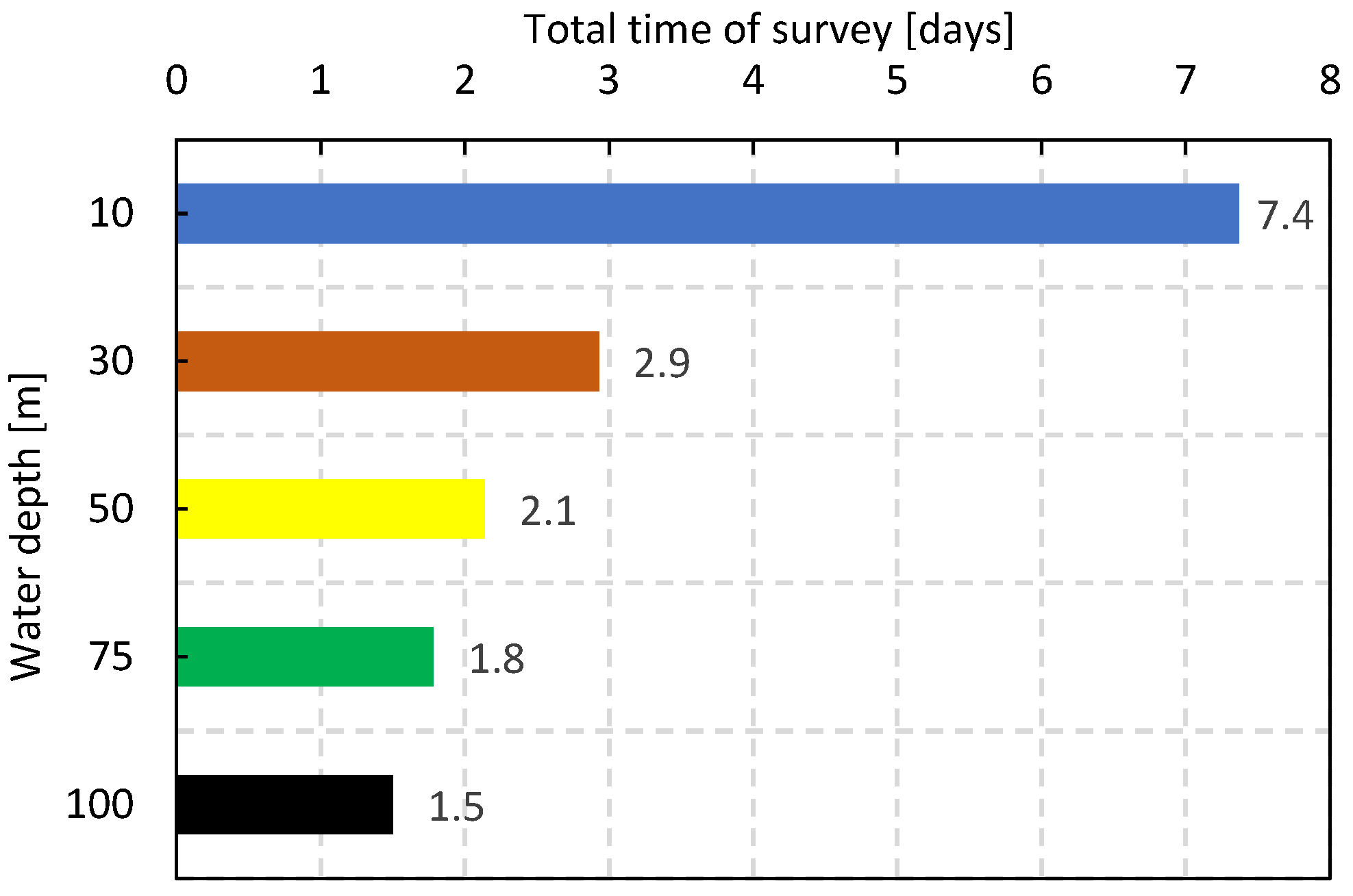
The simulation results of the duration of the survey area with dimensions of 6 × 3 Nm for five different water depths are shown in Figure 4.

Figure 4.
Estimated survey time of the water body of the same area conducted with a multi-beam echosounder for five different depth values (water basin 6 × 3 Nm).
The variables of the depth of survey area determined the use of MBES swath angles in the calculations. For the depth of 10 m, θu = 140° was assumed; for the depth of 50 m, the angle θu = 100° was used; and for the deepest body of water, the angle θu = 70° was substituted. Decreasing MBES swat angles directly affect the change in survey speed. The results of the calculations clearly show that the survey of the shallowest basin, despite setting the widest MBES transmitting sector, will take the most time, i.e., 7.4 days. As the depth increases, the total survey time of the water body of the same area decreases.
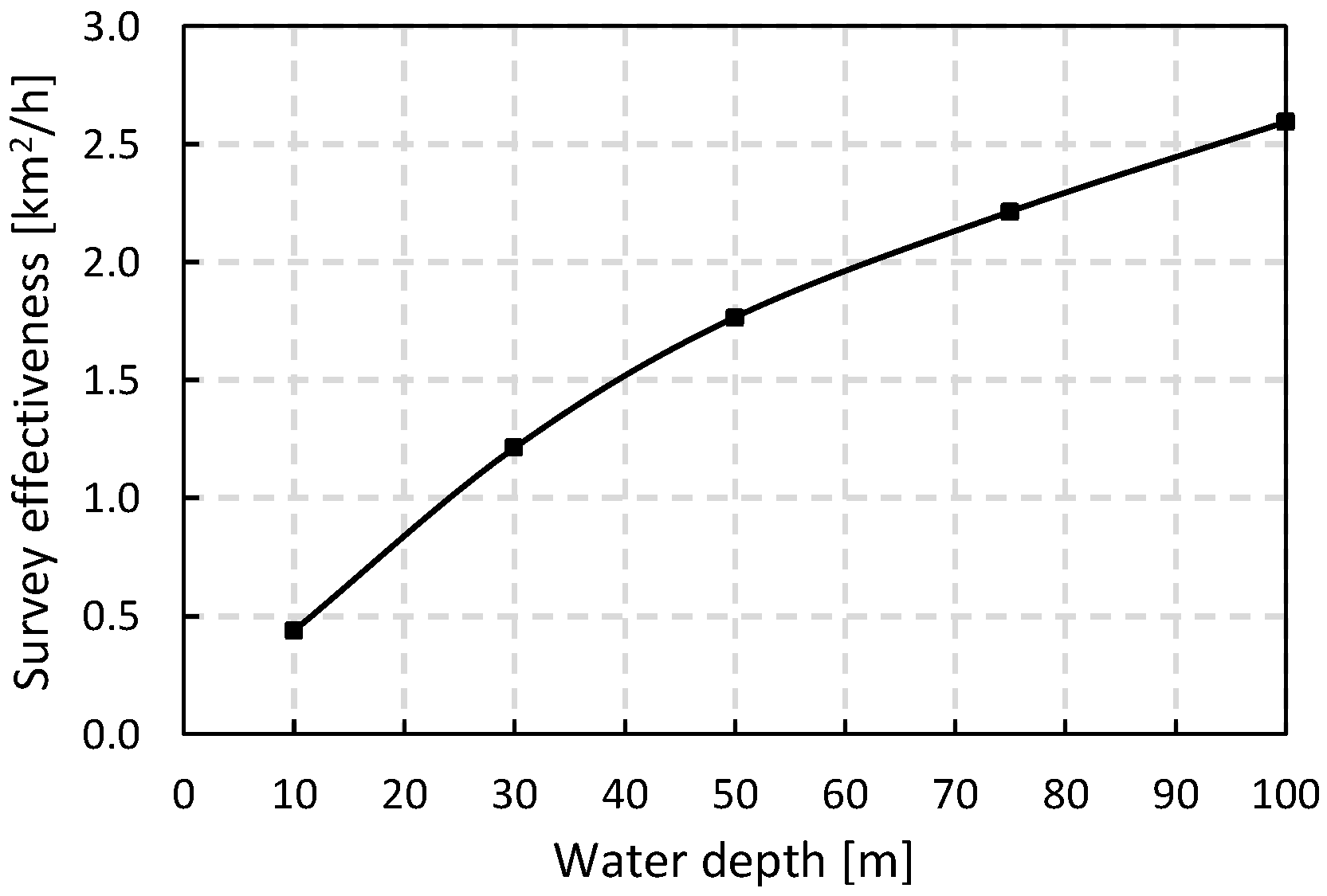
The simulation results (Figure 4) can be used to determine an additional parameter, namely, the so-called hydrographic survey effectiveness Eson. The hydrographic survey effectiveness can be expressed by the ratio of the surveyed water body size to the time unit, i.e., the survey speed of the vessel following survey lines. The speed can be neither arbitrary nor the maximum one. The effectiveness of the hydrographic survey work Eson can be determined as the product of the swath width of the multi-beam echosounder and the maximum speed adopted for the survey:
where: Eson—effectiveness of the hydrographic survey [m2/s]; Vson—maximum vessel’s speed adopted for the survey [m/s]; SW—swath width of the multi-beam echosounder [m]. The swath width of the multi-beam echosounder is calculated using formula no. 5. The results are presented in Table 4.
Table 4.
MBES swath width for five different water depths.
Assuming the useful MBES swath angles values θu, calculated survey speed Vson, and the swath widths of the multi-beam echosounder SW, the hydrographic survey effectiveness was determined and presented in Figure 5.

Figure 5.
Hydrographic survey effectiveness for water bodies of different depth (water area 6 × 3 Nm).
The effectiveness increases with the water depth of the survey area. Very shallow waters, ports, canals, and port basins belong to areas where bathymetric measurements are characterized by low efficiency, which undoubtedly affects the costs that the contractor must incur. The number of survey lines can, of course, be reduced by using wider or maximum MBES swath angles. The survey time in very shallow waters can also be shortened by simply increasing the speed of the vessel. However, there is a risk that when using the hydrographic survey parameters above the allowable rate, the data recorded in this way will not be recognized by the client due to the exceeded total vertical and horizontal uncertainty or the failure to detect all underwater objects.
Most hydrographic offices and commercial companies providing services in the field of survey works assume the maximum MBES swath angle of 120°, and in some reservoirs, even 100° can be assumed [59]. Such an explicit limitation of the beamwidth, on the one hand, affects the efficiency of survey work, and on the other hand, minimizes measurement errors. Questions about the useful angular sector of multi-beam echosounder systems, the swath width, or the survey speed are significant in the case of special-purpose measurements, e.g., mapping the seabed for the purpose of safety of navigation and marine cartography.
3.3. Limitations of the Proposed Method of Survey Time Estimation and Future Research Directions
When surveying with multi-beam echosounder, line spacing is influenced by water depth, data density, and overlap “p”. In real conditions, line spacing will vary across the survey area since the water depth and terrain roughness change. The proposed method assumes the same average depths within the designated survey area, but this will never happen unless a small body of water is involved. If we are dealing with a varied bottom relief, two approaches might be considered. One of the methods of optimal selection of the survey line spacing and overlap is to divide the survey area into two separate water bodies and perform time estimations separately. The second approach is to carefully monitor the recorded depths during the survey operation and respond online by updating the spacing and overlap parameters in the project. The latter method is quite commonly used by practitioners onboard the survey vessels. Some unmanned surface vehicles (USV) are equipped with solutions consisting of autonomous calculation and selection of the line spacing based on current, on-line depth measurements, and the required overlap value.
The quality of the final product of the hydrographic survey is directly related to the accuracy of the depth measurements performed with the multi-beam echosounder. Depth measurement accuracy is not only dependent on the accuracy of the multi-beam echosounder itself; this parameter depends on many factors, mainly on the performance of additional sensors such as the motion sensor, the gyrocompass, the sound velocity profiler, the positioning sensor, the accuracy of sensors’ offsets, and so on. The issue of how different error sources contribute to the final accuracy of data as a function of survey duration is complex. To propose a comprehensive survey planning approach, future work should be focused on the integration of bathymetric data quality alongside time considerations in the survey planning. However, to create such a dependency diagram, actual measurement ought to be performed with the use of a multi-beam echosounder. Such tests could include the acquisition of real depth values on the same sea area (lake) for various settings of MBES swath angles and the estimation of the final depth measurement uncertainty. The studies should be performed at different depths. In this way, a diagram could be created taking into account the requirements of the IHO S-44 standards, the available MBES swath angles, and the time required for performing the hydrographic survey.
4. Conclusions
Hydrographic surveying is a regular and costly activity; hence, careful hydrographic survey planning is required. The aim of this paper was to present the method of time estimation for the bathymetric surveys performed with a multi-beam echosounder. The proposed model involves many variables and parameters that should be taken into account in the time calculation. The article demonstrates how the total survey time changes as a function of several parameters and variables. This is extremely important in the context of planning the costs of maritime operations, which, in fact, depends on the time spent at sea. The results clearly show that the time of measurement work and the effectiveness depend mainly on the depth of the water body, the settings of multi-beam echosounder, and the speed of the vessel. The article also draws attention to the fact that the use of exceeded survey speeds or MBES swath angles may negatively affect the final quality and accuracy of bathymetric data. The selection of these parameters is the measurement contractor’s responsibility and is a subjective matter for the hydrographer liable for planning and executing the survey. The proposed method of calculating the survey time can be successfully used by planners of the National Hydrographic Offices, the Maritime Offices, and institutions and companies dealing with professional measurements in different water environments.
Funding
This research received no external funding.
Institutional Review Board Statement
Not applicable.
Informed Consent Statement
Not applicable.
Data Availability Statement
Not applicable.
Conflicts of Interest
The author declares no conflict of interest.
References
- Mayer, L.A.; Paton, M.; Gee, L.; Gardner, S.V.; Ware, C. Interactive 3-D visualization: A tool for seafloor navigation, exploration and engineering. In Proceedings of the OCEANS 2000 MTS/IEEE Conference and Exhibition, Providence, RI, USA, 11–14 September 2000; Volume 2, pp. 913–919. [Google Scholar]
- Moustier, C. State of the art in swath bathymetry survey systems. IHR 1988, LXV, 25–54. [Google Scholar]
- International Marine Contractors Association IMCA. Guidelines for the Use of Multibeam Echosounder for Offshore Surveys; IMCA S 003 Rev. 2; IMCA: London, UK, 2015. [Google Scholar]
- Morris, G.F. Introducing an Operational Multi-Beam Array Sonar. IHR 1970, XLVII, 35–39. [Google Scholar]
- Pøhner, F. The Evolution of Technology for Multibeam Echo Sounding. Ranger. J. Def. Surv. Assoc. 2005, 2, 15–18. [Google Scholar]
- Mitchell, N.C.; Hughes-Clarke, J.E. Classification of seafloor geology using multibeam sonar data from the Scotian Shelf. Mar. Geol. 1994, 121, 143–160. [Google Scholar] [CrossRef]
- Courtney, R.C.; Shaw, J. Multibeam bathymetry and back-scatter imaging of the Canadian continental shelf. Geoscience 2000, 27, 31–42. [Google Scholar]
- Moustier, C. Beyond bathymetry: Mapping acoustic backscatter from the deep seafloor with Sea Beam. J. Acoust. Soc. Am. 1986, 79, 316–331. [Google Scholar] [CrossRef]
- Preston, J. Acoustic Classification by Sonar. Hydro Int. 2004, 8, 23–25. [Google Scholar]
- Brown, C.J.; Beaudoin, J.; Brissette, M.; Gazzola, V. Multispectral Multibeam Echo Sounder Backscatter as a Tool for Improved Seafloor Characterization. Geosciences 2019, 9, 126. [Google Scholar] [CrossRef]
- Hasan, O.; Smrkulj, N.; Miko, S.; Brunović, D.; Ilijanić, N.; Šparica Miko, M. Integrated Reconstruction of Late Quaternary Geomorphology and Sediment Dynamics of Prokljan Lake and Krka River Estuary, Croatia. Remote Sens. 2023, 15, 2588. [Google Scholar] [CrossRef]
- Wan, J.; Qin, Z.; Cui, X.; Yang, F.; Yasir, M.; Ma, B.; Liu, X. MBES Seabed Sediment Classification Based on a Decision Fusion Method Using Deep Learning Model. Remote Sens. 2022, 14, 3708. [Google Scholar] [CrossRef]
- Todd, B.J.; Fader, G.B.J.; Courtney, R.C.; Pickrill, R.A. Quaternary geology and surficial sediment processes, Browns Bank, Scotian Shelf, based on multibeam bathymetry. Mar. Geol. 1999, 162, 165–214. [Google Scholar]
- Orange, D.L.; Yun, J.; Maher, N.; Barry, J.; Greene, G. Tracking California seafloor seeps with bathymetry, backscatter and ROVs. Cont. Shelf Res. 2002, 22, 2273–2290. [Google Scholar]
- Kostylev, V.E.; Todd, B.J.; Fader, G.B.J.; Courtney, R.C.; Cameron, G. Benthic habitat mapping on the Scotian Shelf based on multibeam bathymetry, surficial geology and seafloor photographs. Mar. Ecol. Prog. Ser. 2001, 219, 121–137. [Google Scholar]
- Díaz, J.V.M. Analysis of Multibeam Sonar Data for the Characterization of Seafloor Habitats. Master’s Thesis, The University of New Brunswick, Saint John, NB, Canada, 1999. [Google Scholar]
- Janowski, L.; Trzcinska, K.; Tegowski, J.; Kruss, A.; Rucinska-Zjadacz, M.; Pocwiardowski, P. Nearshore Benthic Habitat Mapping Based on Multi-Frequency, Multibeam Echosounder Data Using a Combined Object-Based Approach: A Case Study from the Rowy Site in the Southern Baltic Sea. Remote Sens. 2018, 10, 1983. [Google Scholar] [CrossRef]
- David, V.; Mouget, A.; Thiriet, P.; Minart, C.; Perrot, Y.; Le Goff, L.; Bianchimani, O.; Basthard-Bogain, S.; Estaque, T.; Richaume, J.; et al. Species identification of fish shoals using coupled split-beam and multibeam echosounders and two scuba-diving observational methods. J. Mar. Syst. 2023, 241, 103905. [Google Scholar]
- Grządziel, A.; Wąż, M.; Naus, K.; Felski, A. Uncertainty in the measurement of depth with multibeam echosounder. Tech. Transp. Szyn. TTS 2015, 12, 2575–2578. [Google Scholar]
- Ranade, G. Impact of Bathymetric System Advances on Hydrography. National Institute of Oceanography, National Seminar June 2007, Goa, 88–96. Available online: http://drs.nio.org/drs/bitstream/handle/2264/696/Impact_Technnol_Proc_21-22_Jun_2007_Goa.pdf?sequence=2&isAllowed=y (accessed on 27 August 2023).
- Siwabessy, P.; Gavrilov, A.; Duncan, A.; Parnum, I. Statistical analysis of high—Frequency multibeam backscatter data in shallow water. In Proceedings of the Acoustics, Christchurch, New Zealand, 20–22 November 2006. [Google Scholar]
- Cruz, J.D.V.; Vicente, J.; Santos, L. Very Shallow Water Survey—A New Approach; Hydro International: Lemmer, The Netherlands, 2015; Available online: https://www.hydro-international.com/content/article/very-shallow-water-survey-a-new-approach (accessed on 20 August 2023).
- Solana Rubio, S.; Salas Romero, A.; Cerezo Andreo, F.; González Gallero, R.; Rengel, J.; Rioja, L.; Callejo, J.; Bethencourt, M. Comparison between the Employment of a Multibeam Echosounder on an Unmanned Surface Vehicle and Traditional Photogrammetry as Techniques for Documentation and Monitoring of Shallow-Water Cultural Heritage Sites: A Case Study in the Bay of Algeciras. J. Mar. Sci. Eng. 2023, 11, 1339. [Google Scholar] [CrossRef]
- Georgiou, N.; Dimas, X.; Fakiris, E.; Christodoulou, D.; Geraga, M.; Koutsoumpa, D.; Baika, K.; Kalamara, P.; Ferentinos, G.; Papatheodorou, G. A Multidisciplinary Approach for the Mapping, Automatic Detection and Morphometric Analysis of Ancient Submerged Coastal Installations: The Case Study of the Ancient Aegina Harbour Complex. Remote Sens. 2021, 13, 4462. [Google Scholar] [CrossRef]
- Kearns, T.A. Remote Sensing and Multibeam Hydrography. Sea Technol. 2002, 43, 21–27. [Google Scholar]
- Gao, J. Bathymetric mapping by means of remote sensing: Methods, accuracy and limitations. Prog. Phys. Geogr. 2009, 33, 103–116. [Google Scholar]
- Holmes, K.W.; Niel, K.; Baxter, K. Designs for Marine Remote Sampling: A Review and Discussion of Sampling Methods, Layout, and Scaling Issues. CRC for Coastal Zone Estuary and Waterway Management Project CB3: Benthic Biology and Habitat Mapping Task 2.1 Milestone Report. 2004. Available online: https://www.researchgate.net/publication/255663044_Designs_for_marine_remote_sampling_a_review_and_discussion_of_sampling_methods_layout_and_scaling_issues#fullTextFileContent (accessed on 24 August 2023).
- US Army Corps of Engineers. Engineering and Design: Hydrographic Surveying; Publication EM 1110-2-1003; US Army Corps of Engineers: Washington, DC, USA, 2013.
- Oliveira, A.M., Jr.; Hughes Clarke, J.E. Extending the multibeam angular sector to improve seafloor classification. Sea Technol. 2008, 49, 17–19. [Google Scholar]
- Hamilton, T.; Beaudoin, J. Modelling uncertainty caused by internal waves on the accuracy of MBES. IHR 2010, 4, 55–65. [Google Scholar]
- Dinn, D.F.; Loncarevic, B.D.; Costello, G. The effect of sound velocity errors on multibeam sonar depth accuracy. In Proceedings of the IEEE Oceans 95 Conference, San Diego, CA, USA, 9–12 October 1995; pp. 1001–1010. [Google Scholar]
- Eeg, J. On the estimation of standard deviations in multibeam soundings. IHR 2015, 73, 39–51. [Google Scholar]
- International Federation of Surveyors (FIG). Guidelines for the Planning, Execution and Management of Hydrographic Surveys in Ports and Harbours; FIG Publication No 56: Copenhagen, Denmark, 2010; Available online: https://www.fig.net/resources/publications/figpub/pub56/figpub56.asp (accessed on 14 July 2023).
- Lafrance, A. A guide to planning a hydrographic survey. AOLS Ont. Prof. Surv. 1994, 37, 27–31. [Google Scholar]
- IHO C-13. Manual on Hydrography, 1st ed.; International Hydrographic Organization: Monaco City, Monaco, 2011. [Google Scholar]
- Nortrup, D.E. Hydrographic Surveying. In The Surveying Handbook; Brinker, R.C., Minnick, R., Eds.; Springer: Boston, MA, USA, 1995. [Google Scholar] [CrossRef]
- Bowditch, N. The American Practical Navigator; Pub. No. 9; Defense Mapping Agency Hydrographic/Topographic Center: Bethesda, MD, USA, 1995.
- New Zealand Hydrographic Authority. Contract Specifications for Hydrographic Surveys, Version 2.0. June 2016. Available online: https://www.linz.govt.nz/sites/default/files/2022-12/HYSPEC%20v2.0.pdf (accessed on 24 July 2023).
- National Oceanic and Atmospheric Administration. Hydrographic Survey Specifications and Deliverables; Technical Report; U.S. Department of Commerce, National Oceanic and Atmospheric Administration: Washington, DC, USA, 2018. Available online: https://nauticalcharts.noaa.gov/publications/docs/standards-and-requirements/specs/hssd-2018.pdf (accessed on 6 July 2023).
- Canadian Hydrographic Service. Standards for Hydrographic Surveys, 4 ed.; Canadian Hydrographic Service Fisheries and Oceans Canada: 2021. Available online: https://chs.gc.ca/data-gestion/standards-normes/index-eng.html#4_3_2 (accessed on 4 March 2023).
- Manual of Defense Standardization. PDNO-06-A073: Marine Hydrography. In Principles of Data Collection and Presentation of Results; Military Center for Standardization, Quality and Codification: Warsaw, Poland, 2009. [Google Scholar]
- Haga, K.H.; Pohner, F.; Nilsen, K. Testing multibeam echosounders versus IHO S-44 requirements. IHR 2003, 4, 31. [Google Scholar]
- Wati, G.N.; Geldof, J.B.; Seube, N. Error budget analysis for surface and underwater survey system. IHR 2016, 15, 21–45. [Google Scholar]
- Hammerstad, E. The challenges of special order object detection. Sea Technol. 2006, 47, 40–54. [Google Scholar]
- Grządziel, A.; Wąż, M. Estimation of effective swath width for dual-head multibeam echosounder. Annu. Navig. 2016, 23, 173–183. [Google Scholar] [CrossRef]
- Hare, R. Error Budget Analysis for US Naval Oceanographic Office Hydrographic Survey Systems; Final Report for Task 2, FY 01; University of Southern Mississippi: Hattiesburg, MS, USA, 2001; 153p. [Google Scholar]
- Gaida, T.C.; Mohammadloo, T.H.; Snellen, M.; Simons, D.G. Mapping the seabed and shallow subsurface with multi-frequency multibeam echosounders. Remote Sens. 2020, 12, 24. [Google Scholar]
- Mohammadloo, T.H.; Snellen, M.; Amiri-Simkooei, A.; Simons, D.G. Assessment of Reliability of Multi-beam Echo-sounder Bathymetric Uncertainty Prediction Models. In Proceedings of the 5th Underwater Acoustics Conference and Exhibition, Crete, Greece, 30 June–5 July 2019; pp. 783–790. [Google Scholar]
- Hare, R.; Eakins, B.; Amante, C. Modelling bathymetric uncertainty. IHR 2011, 6, 31–42. [Google Scholar]
- Hare, R.; Godin, A.; Mayer, L. Accuracy Estimation of Canadian Swath (Multibeam) and Sweep (Multi-Transducer) Sounding Systems; Technical Internal Report; Canadian Hydrographic Service: Ottawa, ON, Canada; University of New Brunswick: Fredericton, NB, Canada, 1995. [Google Scholar]
- Lurton, X. Theoretical Modelling of Acoustical Measurement Accuracy for Swath Bathymetric Sonars. IHR 2003, 4, 17–30. [Google Scholar]
- Buchanan, C.; Spinoccia, M.; Picard, K.; Wilson, O.; Sexton, M.J.; Hodgkin, S.; Parums, R.; Siwabessy, P.J.W. Standard Operation Procedure for a Multibeam Survey: Acquisition & Processing; Record 2013/33; Geoscience Australia: Canberra, Australia, 2013; p. 24. ISBN 978-1-922201-68-3.
- Hare, R. Depth and position error budgets for multibeam echosounding. IHR 1995, LXXII, 37–69. [Google Scholar]
- Pereira, D.J.; Hughes Clarke, J.E. Improving shallow water multibeam target detection at low grazing angles. In Proceedings of the US Hydrographic Conference, National Harbor, MD, USA, 16–19 March 2015. [Google Scholar]
- Kammerer, E. New Methods for Removal of Refraction Artifacts in Multibeam Echosounder Systems. Ph.D. Thesis, The University of New Brunswick, Saint John, NB, Canada, June 2000; 220p. [Google Scholar]
- Cartwright, D. Multibeam Bathymetric Surveys in the Fraser River Delta, Managing Severe Acoustic Refraction Issues. Master’s Thesis, The University of New Brunswick, Saint John, NB, Canada, August 2003. [Google Scholar]
- Grządziel, A. The Impact of Multibeam Echosounder Swath Angle on the Hydrographic Survey Accuracy. Ph.D. Dissertation, Polish Naval Academy, Poland, Gdynia, 2019. [Google Scholar]
- S-44 Edition 6.1.0; IHO Standards for Hydrographic Surveys, Special Publication No 44. IHO: Monaco, Monaco, 2022.
- Thain, R.H.C. The Dynamics of Tidal Intrusion Front in a Natural Estuary: Effects on Multibeam Sonar Accuracy. Ph.D. Thesis, University of Plymouth, Plymouth, UK, 2005; 270p. [Google Scholar] [CrossRef]

Disclaimer/Publisher’s Note: The statements, opinions and data contained in all publications are solely those of the individual author(s) and contributor(s) and not of MDPI and/or the editor(s). MDPI and/or the editor(s) disclaim responsibility for any injury to people or property resulting from any ideas, methods, instructions or products referred to in the content. |
© 2023 by the author. Licensee MDPI, Basel, Switzerland. This article is an open access article distributed under the terms and conditions of the Creative Commons Attribution (CC BY) license (https://creativecommons.org/licenses/by/4.0/).