Physically-Data Driven Approach for Predicting Formation Leakage Pressure: A Dual-Drive Method

Abstract

Formation leak-off pressure, which sets the upper limit of the safe drilling fluid density window, is crucial for preventing wellbore accidents and ensuring safe and efficient drilling operations. The paper thoroughly examines models of drilling physics alongside artificial intelligence techniques. The study introduces a dual-driven method for predicting reservoir pore pressure by integrating long short-term memory (LSTM) and backpropagation (BP) neural networks, where the core component is the LSTM-BP neural network model. The input data for the LSTM-BP model include wellbore diameter, formation density, sonic time, natural gamma, mud content, and pore pressure. The study demonstrates the practical application of the method using two vertical wells in Block M, employing the M-1 well for training and the M-2 well for validation. Two distinct input layer configurations are devised for the LSTM-BP model to evaluate the influence of formation density on prediction accuracy. Notably, Scheme 2 omits formation density as a variable in contrast to Scheme 1. The study’s results indicate that, for input layer configurations corresponding to Scenario 1 and Scenario 2, the LSTM-BP model exhibits relative error ranges of (−2.467%, 2.510%) and (−6.141%, 5.201%) on the test set, respectively. In Scenario 1, the model achieves mean squared error (MSE), mean absolute error (MAE), and R-squared (R²) values of 0.000229935, 0.011198329, and 0.92178272, respectively, on the test set. Conversely, for Scenario 2, the model demonstrates a substantial escalation of 992.393% and 240.674% in MSE and MAE, respectively, compared to Scenario 1; however, R² diminishes by 66.920%. Utilizing the trained LSTM-BP model, predictions for formation lost pressure in Well M-2 reveal linear correlation coefficients of 0.8173 and 0.6451 corresponding to Scenario 1 and Scenario 2, respectively. These findings imply that the predictions from the Scenario 1 model demonstrate stronger alignment with results derived from formulaic calculations. These observations remain consistent for both the BP neural network algorithm and the random forest algorithm. The aforementioned research results not only highlight the elevated predictive precision of the LSTM-BP model for intelligent prediction of formation lost pressure, a product of this study, thereby furnishing valuable data points to enhance the security of drilling operations in Block M, but also underscore the necessity of deliberating both physical relevance and data correlation during the selection of input layer variables.

1. Introduction

Drilling operations entail the occurrence of drilling fluid leakage into the formation through cracks (referred to as leakage channels) in the wellbore. This occurrence is commonly known as wellbore leakage. Wellbore leakage has an estimated global annual occurrence rate of approximately 25%, resulting in costs exceeding USD 4 billion for mitigation [1]. Wellbore leakage has emerged as a prevalent issue in drilling operations [2].

Wellbore leakage is a highly complex phenomenon influenced by multiple factors, such as formation properties, drilling fluid properties, drilling construction processes, and underground pressure variations [3]. Formation properties, such as rock permeability, porosity, and fractures, play a significant role in influencing the formation leakage pressure. Drilling fluid properties, particularly density and viscosity, have a direct impact on the incidence of wellbore leakage. Stress changes in the wellbore, induced by the rotation and fluctuating pressure of the drill bit during the drilling process, can lead to wellbore leakage. Wellbore leakage is a frequent and intricate subterranean incident that frequently occurs abruptly and necessitates a complex subsequent remediation process. Wellbore leakage results in the wastage of manpower and resources, along with substantial increases in drilling time and costs. In severe instances, wellbore leakage can result in blowouts, surges, or even necessitate wellbore abandonment [4].

Precise prediction of formation leakage pressure plays a crucial role in mitigating wellbore leakage [5]. Formation leakage pressure denotes the maximum pressure threshold that the wellbore can sustain under wellbore leakage conditions and serves as the upper limit for designing a safe drilling fluid density range. Investigating formation leakage pressure holds immense significance in ensuring drilling operation safety, optimizing drilling fluid performance, reducing costs, safeguarding reservoir integrity, enhancing drilling construction efficiency, and informing wellbore structural design.

With the deepening of oil and gas exploration and development, research on leakage pressure has steadily progressed. In 1990, N. Morita introduced the theory of leakage pressure and conducted an analysis of its influencing factors [6]. In 2004, Alexandre Lavrov pioneered the development of a leakage pressure model suitable for fractured formations [7]. In 2010, Majidi et al. developed a drilling fluid leakage model for naturally fractured formations using the Herschel–Bulkley rheological model [8]. They emphasized the importance of controlling the drilling fluid’s rheology to minimize losses. Presently, numerous scholars have extensively researched various disciplines, such as geomechanics, wellbore stability, and fluid mechanics. Research methodologies encompass numerical simulation, laboratory experiments, and field observations. In recent decades, researchers have developed numerous mathematical models and empirical formulas to predict formation leakage pressure based on extensive experimental investigations and theoretical analyses. However, the applicability of these methods is limited due to the multitude of causes and complex mechanisms of wellbore leakage, resulting in the absence of a universally applicable theoretical calculation model for leakage pressure [9]. Presently, the methods used to predict formation leakage pressure primarily involve experimental analysis [5], numerical simulation [10], theoretical formulas [11], empirical formulas [9], and statistical analysis [5].

Currently, the predominant approach for determining formation leakage pressure is primarily based on understanding the leakage mechanism. It involves analyzing leakage scenarios in the target formation using statistical data and relevant empirical formulas derived from drilled wells [12]. However, in reality, wellbore leakage is influenced by numerous causes and intricate mechanisms, and the actual conditions vary among different geological formations. Consequently, it is challenging to formulate a universally applicable calculation formula, as theoretical formulas rely on specific assumptions that might not completely align with the actual drilling conditions. Consequently, the calculated results offer limited guidance for onsite operations and pose challenges when attempting to generalize and apply them [13]. Conventional empirical formulas face challenges in accurately determining empirical coefficients, and the selection of empirical parameters is highly subjective. Conversely, statistical models demand substantial preliminary statistical work and might not fulfill the practical requirements for leakage prevention, particularly in newly developed blocks with limited relevant data and absence of reference methods. Presently, a pressing need exists for a relatively universal calculation method for accurately predicting formation leakage pressure. Such a method should enhance prediction accuracy, improve computational efficiency, and reduce operational costs.

In recent years, due to the ongoing advancements in artificial intelligence technology, the extensive research and application of artificial intelligence have become prevalent across various industries [14,15]. It offers notable advantages in addressing intricate nonlinear problems. Within the petroleum sector, the utilization of machine learning techniques for the advancement of both conventional and unconventional oil and gas fields is progressively gaining traction [16]. An increasing number of scholars are embarking on investigations into the application of artificial intelligence methods, such as machine learning and deep learning, for in-depth analyses of mechanisms and patterns related to well leakage [17]. For instance, Sabah et al. [18] collected data from 61 wells in the Marun oilfield in Iran to predict wellbore leakage. The dataset comprised 19 parameters, including well depth, drilling pressure, and drill bit rotation speed, resulting in a total of 1900 data points. They employed algorithms like artificial neural networks (ANNs), support vector machines (SVMs), and decision trees to develop a model for predicting wellbore leakage. The model’s performance was assessed using evaluation metrics like root mean square error (RMSE) and coefficient of determination (R²). Geng et al. [19] identified the four most highly correlated parameters, namely, variance, attenuation, sweetness, and RMS amplitude, from a set of 15 seismic attribute parameters. They presented a predrilling method for assessing wellbore leakage risk using machine learning techniques and three-dimensional seismic data. Pang et al. [20] identified 16 out of 22 comprehensive logging parameters that were most pertinent to drilling fluid leakage. They utilized the mixture density network to evaluate and forecast drilling fluid leakage. Li et al. employed three machine learning algorithms, specifically artificial neural networks (BPNN), support vector machines (SVMs), and random forests, to predict wellbore leakage [21]. They utilized 12 parameters, including well depth, drilling fluid density, and pore pressure, as input for the models. The investigation determined that the random forest algorithm achieved the highest performance. These examples underscore the growing adoption of machine learning and artificial intelligence methods in studying and predicting wellbore leakage, promising enhanced accuracy and efficiency in the analysis and prevention of such incidents.

In the context of leak-off speed prediction, Jahanbakhshi et al. [22] utilized artificial neural networks (ANNs) to develop two models for predicting leak-off speed in natural fractured formations. In the first model (Scheme 1), the input layer parameters comprised conventional drilling parameters, including well depth, porosity, and formation permeability. In the second model (Scheme 2), additional geomechanical parameters, such as Young’s modulus, were incorporated in addition to those in Scheme 1. The results demonstrated that Scheme 2 exhibited lower errors, signifying its superior performance. Hou et al. utilized the South China Sea region as a case study and developed a leak-off type prediction model based on the division of leak-off speed [23]. The model employed artificial neural networks (ANNs) and big data techniques, utilizing formation properties, drilling parameters, and drilling fluid parameters as input variables. The model achieved a prediction accuracy rate of 92% in assessing wellbore leakage risk.

In the domain of wellbore leakage monitoring and early warning, Unrau et al. devised a detection model for early wellbore leakage warning using real-time drilling data from 132 wells [24]. Multiple machine learning algorithms were employed to establish the model, which achieved a false alarm rate of only once every 5 h for wellbore leakage. Andia et al. developed a software solution named RSFMc for early wellbore leakage warning [25]. The software integrates real-time drilling data with diverse artificial intelligence algorithms and offers visual representation of multiple data aspects, including formation pore pressure, fracture pressure, and bottom hole pressure profiles. Additionally, it enables real-time monitoring of wellbore leakage. These examples illustrate the utilization of machine learning and artificial intelligence algorithms in the development of early warning systems for wellbore leakage. These systems capitalize on real-time drilling data to deliver precise and timely alerts, thereby improving the safety and efficiency of drilling operations.

Presently, there is a substantial body of research focusing on the utilization of artificial intelligence techniques in conjunction with seismic, logging, and drilling data to forecast formation permeability and leak-off speed, and enable wellbore leakage monitoring and early warning. However, there is a dearth of articles that directly employ artificial intelligence methods for the prediction of formation leakage pressure. To address this research gap, the present study introduces a method that combines physics-based models and data-driven approaches to predict formation leakage pressure. The detailed workflow is illustrated in Figure 1.

Drawing upon geomechanical theory and expert knowledge, six logging data parameters (CAL, DT, GR, VSH, Pp, and DEN) are chosen as input parameters for the model. Recognizing the presence of sequence dependency in logging data and the effectiveness of long short-term memory (LSTM) networks in managing long sequences, an LSTM-BP neural network model is developed. Spearman correlation analysis is employed to examine the correlation between the six input parameters and formation leakage pressure. Two distinct input layer schemes are devised, and for each scheme, separate modeling, training, analysis, and evaluation are performed. By integrating geological and engineering knowledge into the machine learning model, the objective is to constrain the model’s predictions and enhance the reliability of formation leakage pressure forecasts, ensuring alignment with geological and engineering principles. This research plays a vital role in streamlining the prediction process of formation leakage pressure, enhancing prediction accuracy, expanding the applicability and feasibility of prediction methods, and advancing intelligent drilling engineering.

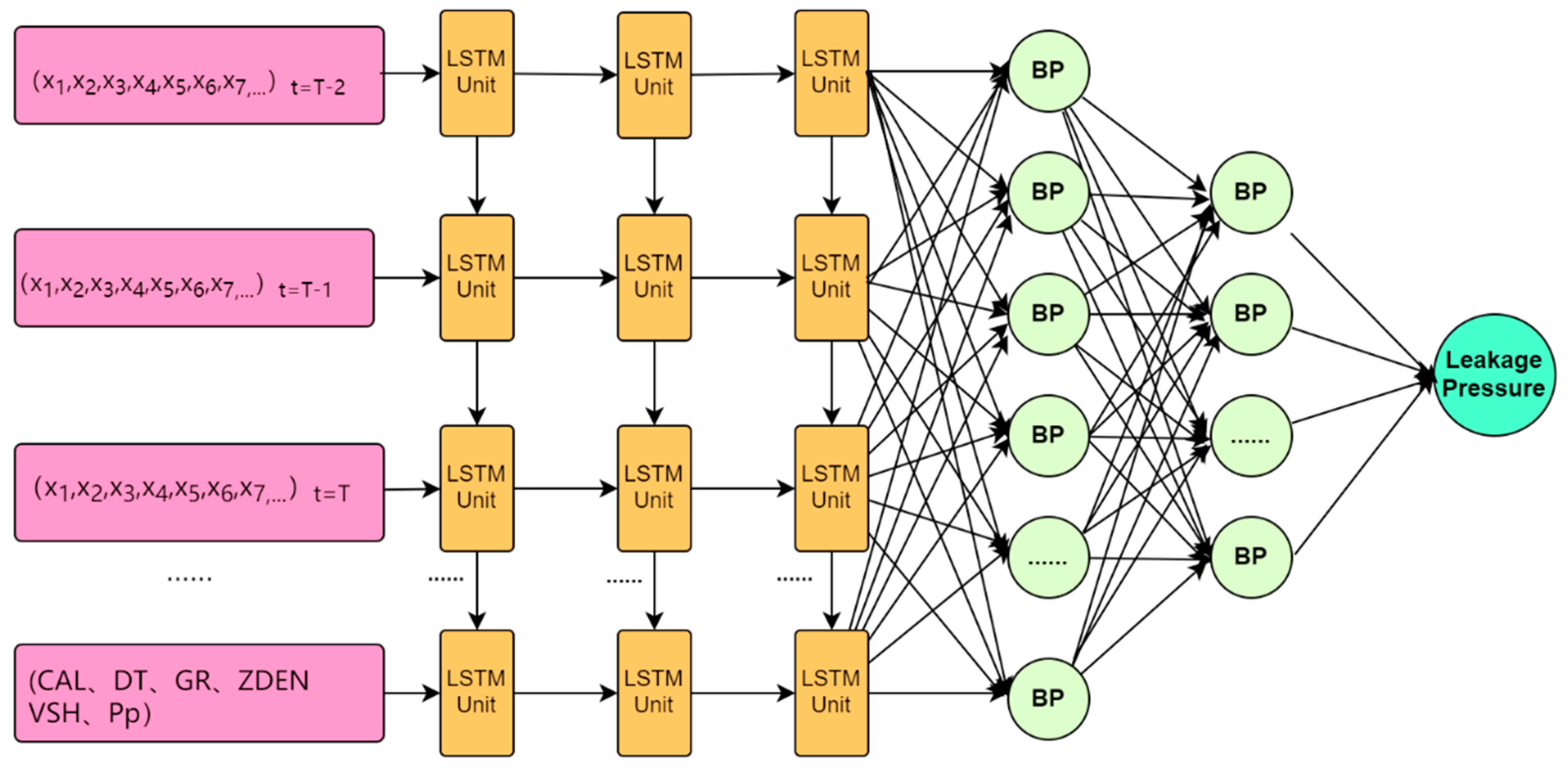
2. Theory and Methods

2.1. LSTM Algorithm Theory

LSTM (long short-term memory) is an enhanced algorithm derived from the RNN (recurrent neural network) [26]. It offers notable advantages in solving long sequence memory problems, facilitating better gradient propagation, and mitigating the problems of gradient vanishing or exploding. Consequently, these advantages position it as a pivotal technology in domains like natural language processing and speech recognition [27]. In comparison to traditional RNN, LSTM exhibits several noteworthy advantages:

(1)

Long-term dependencies: Traditional RNNs encounter challenges in managing long sequence dependencies, whereas LSTM can preserve long-term dependencies by regulating the flow of information.

(2)

Avoiding gradient vanishing or exploding: Traditional RNNs are susceptible to the issues of gradient vanishing or exploding, whereas LSTM incorporates gate mechanisms to regulate the flow of information, effectively mitigating these problems.

(3)

Enhanced memory capacity: LSTM can selectively retain or discard past information through the control of the forget gate and input gate, thereby exhibiting improved memory capabilities.

(4)

Learning patterns in long sequences: LSTM can acquire patterns in long sequences by regulating the flow of information, facilitating superior processing of long sequence data.

In conclusion, LSTM surpasses traditional RNN in its handling of long-term dependencies, ability to avoid gradient vanishing or exploding, improved memory capacity, and proficiency in learning patterns within long sequences.

For a comprehensive depiction of the fundamental network structure of LSTM, please consult Figure 2. Its fundamental concept is rooted in extensive research on cell states and “logic gates”. The cell state serves as the conduit for information transmission, facilitating the transfer of information across the sequence chain and functioning as the network’s “memory”. In theory, the cell state can persistently convey pertinent information throughout sequence processing, allowing information from earlier time steps to be propagated to subsequent time steps, thereby surpassing the constraints of short-term memory. In terms of information control, LSTM accomplishes this through a structure known as “gate logic”. During the training process, the “logic gates” selectively retain or discard information based on their respective weights. The gate logic primarily encompasses the forget gate, input gate, and output gate, each fulfilling distinct functions [28,29]. The forget gate regulates the retention or omission of the preceding layer’s concealed cell state. The input gate evaluates the current input data to ascertain its relevance for updating the cell state. The output gate determines the value of the subsequent hidden state, encompassing the preceding input information [30]. The specific calculation formula is presented as Equation (1).

$$\begin{array}{l}{\mathit{f}}_t=sigmoid\left({\mathit{W}}_{\mathit{f}}\cdot \left[{\mathit{h}}_{t-1},{\mathit{x}}_t\right]+{\mathit{b}}_f\right)\\ {\mathit{i}}_t=sigmoid\left({\mathit{W}}_i\cdot \left[{\mathit{h}}_{t-1},{\mathit{x}}_t\right]+{\mathit{b}}_i\right)\\ {\mathit{o}}_t=sigmoid\left({\mathit{W}}_o\cdot \left[{\mathit{h}}_{t-1},{\mathit{x}}_t\right]+{\mathit{b}}_o\right)\\ {\tilde{\mathit{C}}}_t=\tan h\left({\mathit{W}}_C\cdot \left[{\mathit{h}}_{t-1},{\mathit{x}}_t\right]+{\mathit{b}}_c\right)\\ {\mathit{C}}_t={\mathit{f}}_t\cdot {\mathit{C}}_{t-1}+{\mathit{i}}_t\cdot {\tilde{\mathit{C}}}_t\\ {\mathit{h}}_t={\mathit{o}}_t\cdot \tan h\left({\mathit{C}}_t\right)\end{array}$$

(1)

In the equation:

${\mathit{f}}_t$,${\mathit{i}}_t$, and ${\mathit{o}}_t$ represent the output vectors corresponding to the forget gate, input gate, and output gate, respectively;

${\mathit{W}}_f$,${\mathit{W}}_i$,${\mathit{W}}_o$ are weight matrices corresponding to each gate;

${\mathit{b}}_f$,${\mathit{b}}_i$,${\mathit{b}}_o$ are the offset vectors with each gate;

Sigmoid and tanh are activation functions;

${\mathit{W}}_C$ and ${\mathit{b}}_c$ are weight matrix and bias vector corresponding to the cell state;

${\mathit{h}}_{t-1} \mathrm{and} {\mathit{x}}_t$ are the concatenated results of the previous time step output vector h_(t−1) and the current time step input vector x_t;

${\mathit{C}}_t$ and ${\mathit{C}}_{t-1}$ are the cell state vectors at time step t and t − 1, respectively;

${\tilde{\mathit{C}}}_t$ represents the candidate memory cell matrix;

${\mathit{h}}_t$ is the output vector of the cell block at time step t.

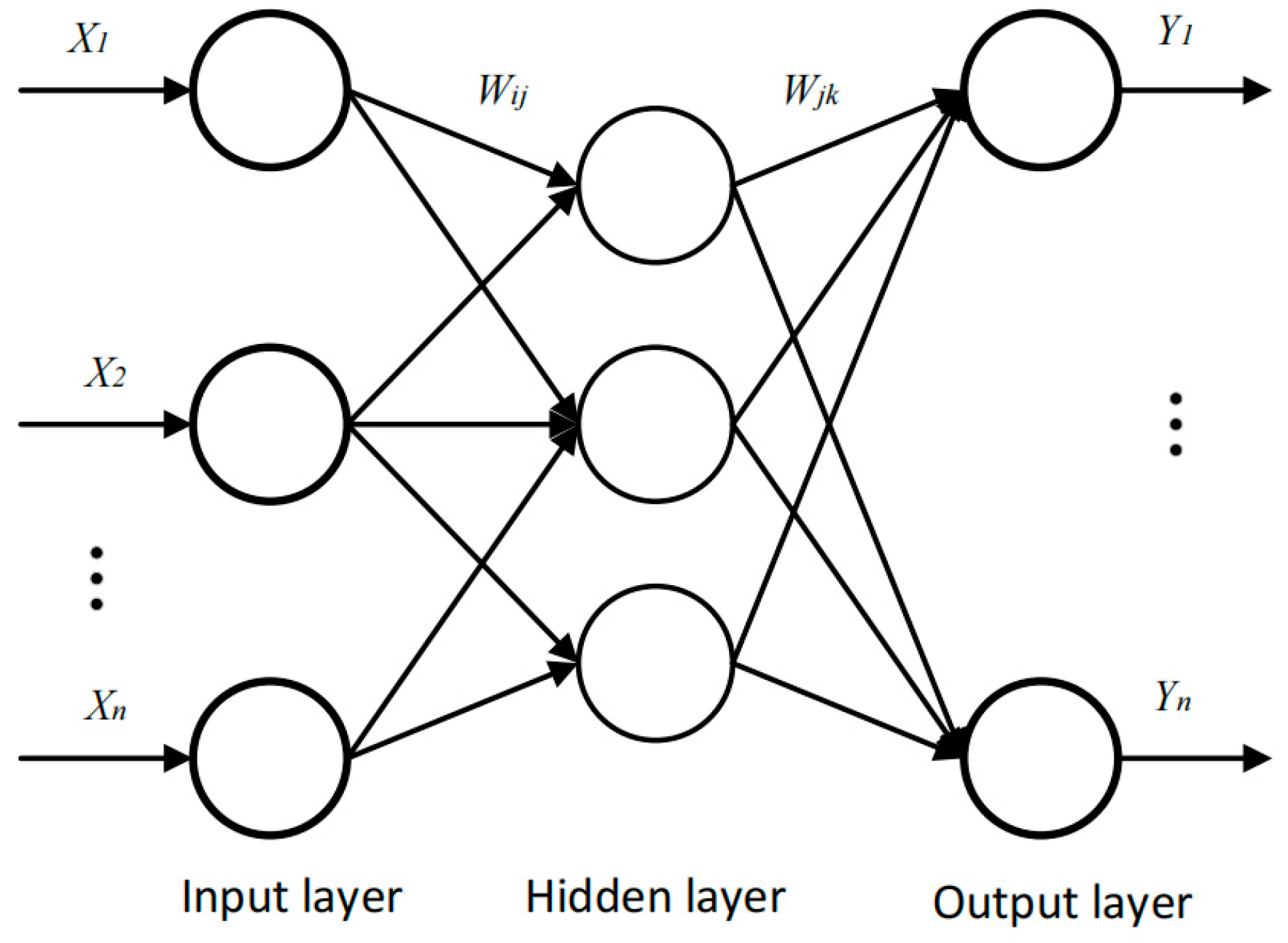
2.2. Backpropagation Neural Network Algorithm

The backpropagation (BP) neural network algorithm, commonly referred to as the error backpropagation algorithm, was introduced by American scientist Rumelhart in 1986 [31]. Presently, it stands as one of the most widely employed and effective algorithms, finding extensive applications in fields such as signal processing, pattern recognition, and intelligent control. The BP neural network comprises multiple layers, including the input layer, output layer, and hidden layer. Connections exist only between layers, with no connections within the same layer, thus forming a fully connected structure. The structure of the BP neural network is depicted in Figure 3. The dataset X = {x₁, x₂,…, x_n} is derived by extracting features from a substantial amount of known data, while the corresponding predicted output values for each data point are denoted by Y = {y₁, y₂,…, y_n}. In the learning process of the neural network, a nonlinear layer, referred to as the hidden layer, is formed. During the training process, the generated errors are iteratively propagated from the hidden layer to the input layer, facilitating the adjustment of unit weights, a process commonly referred to as backpropagation.

3. Selection, Processing, and Correlation Analysis of Training Samples

3.1. Overview of Data Sources

The research data for this study are obtained from two vertical wells, Well M-1 and Well M-2, located in Block M. Well M-2 is situated approximately 6.7 km southwest of Well M-1. Figure 4 illustrates a lithostratigraphic comparison between the two wells. Sequentially, the M block drills through formations A, B, C, and D. Formation C pertains to the principal oil and gas development stratum within this block, primarily characterized by gray and sandy mudstone, intercalated with multiple thin coal seams. The M block exhibits a complex internal structural configuration, featuring well-developed, deep-seated faults. Faulting has led to the fragmentation of the reservoir into isolated blocks. The internal fault structure displays pronounced heterogeneity, characterized by localized stress concentration and varying stress fields. The substantial drilling depth within this block results in a complex vertical lithological profile. The shallow sections comprise readily hydratable mudstone, whereas the middle and deeper sections consist of hard, brittle mud shale. These formations are susceptible to wellbore collapse, leading to intricate challenges such as sticking. The occurrence of faults, coal–rock interlayers, or fractured formations during drilling increases the likelihood of leakage. Consequently, these sections become zones of high drilling risk. Statistical data from prior drilled wells indicate that among the 35 wells within the M block, 13 wells encountered leaks, constituting 37.14% of the total. Additionally, the presence of abnormally high formation pressures in the middle and deeper sections constrains the safety window for drilling operations. Designing drilling fluid density using conventional formulaic approaches poses challenges.

3.2. Selection of Input Layer Data

For this study, Well M-1 is chosen as the training well to supply sample data for model learning, while Well M-2 serves as the validation well to predict and assess the accuracy and generalization of the trained model. The quality of the sample data has a direct impact on the accuracy of the prediction results. This study establishes an intelligent prediction model for pressure loss by selecting specific logging data from Well X-1, guided by the fundamental principles of formation pressure loss and existing research findings. The input layer data of the prediction model comprise well diameter (CAL), formation density (DEN), sonic travel time (DT), natural gamma (GR), shale content (VSH), and equivalent pore pressure density (Pp). This selection is grounded in the capability of logging data to directly capture essential information about the formations, along with its attributes of continuity, accuracy, and cost-effectiveness, which render it a crucial foundation for subsequent developmental endeavors.

The logging data selected as input parameters are visualized using a violin plot, as depicted in Figure 5. Within the violin plot, the median is represented by a central dot, the boxplot illustrates the data spanning from the lower quartile to the upper quartile, the black lines indicate data points within 1.5 times the interquartile range, and the outer shape depicts the kernel density estimate. Figure 5 reveals that the distribution of each input parameter does not conform to a standard normal distribution. Hence, subsequent correlation analysis should utilize Spearman correlation analysis. Additionally, the absence or scarcity of outliers in the data suggests the rational construction of the dataset.

3.3. Data Preprocessing

Preprocessing is essential prior to formally establishing the model due to the presence of substantial noise in the raw logging data, especially noticeable in outliers at the beginning and end, as well as some missing values. This process includes replacing or eliminating the outliers to enhance the quality of the training samples. For this study, the output layer data employed in model training (i.e., the formation pressure loss equivalent density of Well M-1) is computed by domain experts using a formula (refer to Equation (2)) and fine-tuned through calibration considering field conditions and years of experience. Consequently, it demonstrates a high level of accuracy and can be regarded as the actual formation pressure loss. For more details, please consult Figure 6.

$$P_l=\mathrm{a}\ast P_{smin}$$

(2)

In the equation, P_l denotes the formation pressure loss, measured in MPa. The variable “a” is a dimensionless empirical coefficient that pertains to the region, while “P_smin” corresponds to the minimum horizontal principal stress, expressed in MPa.

The primary focus of this research is on the B Formation, C Formation, and D Formation in Block M. Following data preprocessing, Well M-1 covers a depth interval of 2127 to 4652 m, whereas Well M-2 spans from 2510 to 4770 m. In both instances, data were gathered at 5 m intervals to assemble the dataset, amounting to 506 rows for Well M-1 and 453 rows for Well M-2.

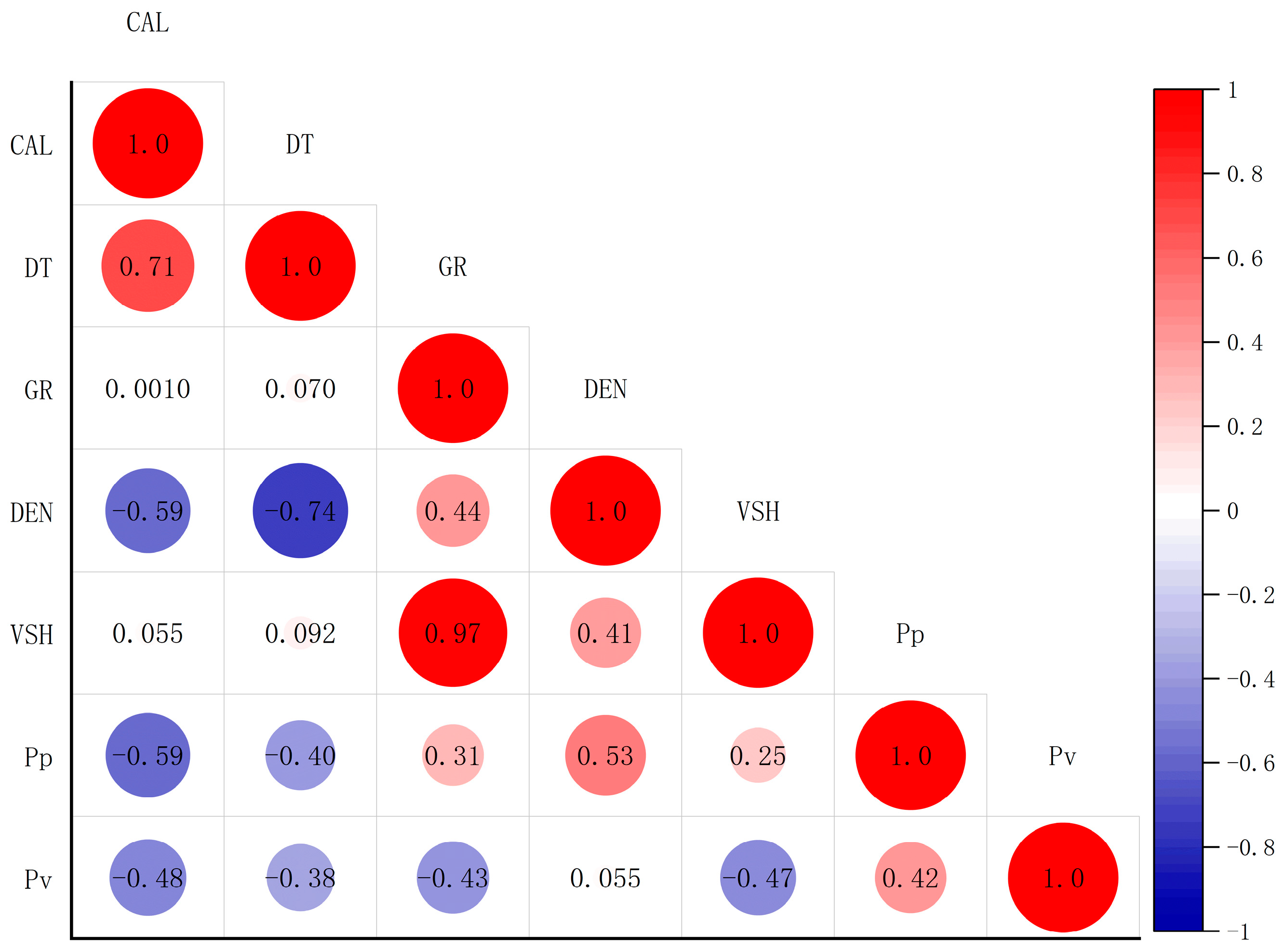
3.4. Data Correlation Analysis and the Setting of Two Models

The previous literature commonly utilizes correlation analysis, particularly Pearson correlation analysis, to select input layer data. Such correlation analyses generally rely on a straightforward mapping relationship between a particular type of data and the output layer data to assess the degree of correlation; however, these analyses do not take into account the underlying mechanism of the data. Hence, in this study, we initially examine the correlation between the selected input layer data and the output layer data, considering a single mapping relationship. Moreover, given that logging data frequently display non-normal distributions (as confirmed in Figure 3), Spearman correlation analysis is employed, as it is appropriate for non-normally distributed data [32]. The degree of correlation is determined by assessing the magnitude of the correlation coefficient. For additional information, please consult Figure 7.

This study computed the p-values for the chosen input layer variables and the formation’s leak-off pressure. All computed p-values were below 0.0001, signifying significant distinctions between the designated feature variables and the leak-off pressure. Consequently, additional scrutiny of the feature variables is imperative to select suitable input layer variables for the model. The analysis of Figure 7 reveals the correlation patterns between the input layer parameters and the formation pressure loss equivalent density (Pv), as follows: In terms of positive or negative correlation, the formation density (DEN) and equivalent pore pressure density (Pp) exhibit a positive correlation with the formation pressure loss equivalent density (Pv). Conversely, well diameter (CAL), sonic travel time (DT), natural gamma (GR), and shale content (VSH) display a negative correlation with the formation pressure loss equivalent density (Pv).

When examining the absolute values of the correlation coefficients, the formation density (DEN) exhibits the weakest correlation with a coefficient of only 0.065. Well diameter (CAL) demonstrates the strongest correlation with the formation pressure loss equivalent density (Pv), followed by shale content (VSH), with both parameters displaying comparable correlation coefficients. Natural gamma (GR) and equivalent pore pressure density (Pp) exhibit slightly lower correlation coefficients, yet their absolute values remain relatively similar.

Based on the aforementioned analysis, when considering the individual correlation [33] between each input layer parameter and the formation pressure loss equivalent density (Pv), well diameter (CAL), natural gamma (GR), shale content (VSH), and equivalent pore pressure density (Pp) demonstrate a moderate correlation, while sonic travel time (DT) displays a weak correlation, and formation density (DEN) exhibits no correlation. However, from a rock mechanics perspective, there exists a certain degree of association between formation density and pressure loss. Therefore, during the subsequent model construction, two different approaches will be considered:

Scheme 1 involves retaining the formation density (DEN) data as an input layer parameter, including CAL, DT, GR, VSH, Pp, and DEN.

Scheme 2 entails removing the formation density (DEN) data as an input layer parameter, consisting of CAL, DT, GR, VSH, and Pp.

A comparative analysis will be conducted between the two approaches during the subsequent training process to evaluate their respective performances.

To mitigate the problem of gradient vanishing or exploding, it is imperative to normalize all sample data, thereby reducing dimensionality and mitigating the impact of varying parameter scales on model performance. Taking into account that drilling is a depth-dependent sequential process and based on the analysis in Figure 5, it is evident that the distribution of the training sample data deviates from a normal distribution. Consequently, the min–max normalization method is employed in this study to normalize the input and output layer data. The normalization equation is defined as Equation (3):

$${\tilde{X}}_i=\frac{X_i-\min \left(X_i\right)}{\max \left(X_i\right)-\min \left(X_i\right)}$$

(3)

where ${\tilde{X}}_i$ is the normalized result of the i-th variable using the min–max normalization method, and the normalized range is [0, 1]. X_i is the original value of the i-th variable, min(X_i) is the minimum value of the i-th variable, and max(X_i) is the maximum value of the i-th variable.

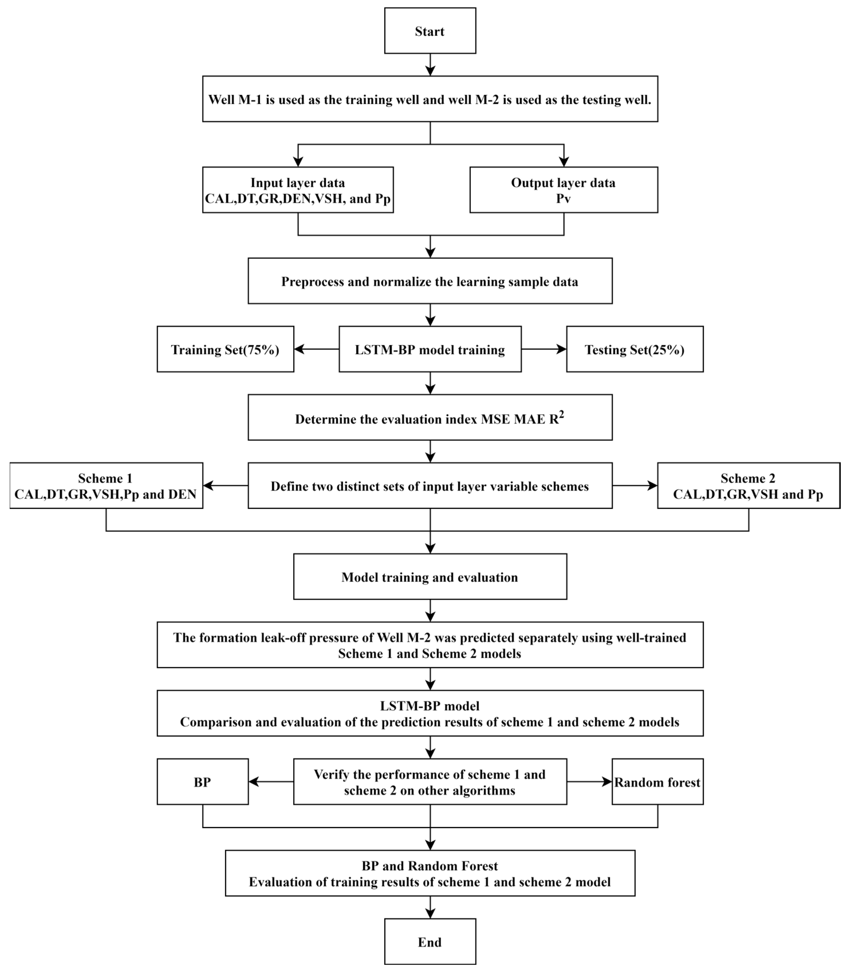
4. Construction, Evaluation, and Application of Intelligent Prediction Models for Formation Pressure Loss

4.1. Model Parameter and Evaluation Metric Settings

The LSTM-BP model in this study is constructed by integrating the LSTM and BP models. For the LSTM-BP model, the input sample sequence length is defined as 3, indicating that it is trained to predict the formation pressure loss at a specific point using the data from the preceding 15 m. Further details regarding the model’s parameter settings are provided in

Table 1. LSTM-BP model parameter table.

NO	Parameters	Value
1	Model layers	3
2	Number of neurons per layer	30
3	Activation function	LeakyRelu
4	Loss function	MSE
5	Maximum number of iterations (epoch)	300
6	Batch size	50
7	Data partitioning	Randomly select 75% of the data as the training set and 25% of the data as the test set.

. The evaluation metrics employed include MSE (mean squared error), MAE (mean absolute error), and R² (coefficient of determination). The relevant formulas for computing these metrics are presented in Equations (4)–(6).

$$\mathrm{M}\mathrm{S}\mathrm{E}=\frac{1}{S}\sum _{i=1}^S {\left(y_i-{\widehat{y}}_i\right)}^2$$

(4)

$$\mathrm{M}\mathrm{A}\mathrm{E}=\frac{1}{\mathrm{S}}\sum _{\mathrm{i}=1}^{\mathrm{S}} \left|{\widehat{y}}_{\mathrm{i}}-{\mathrm{y}}_{\mathrm{i}}\right|$$

(5)

$$R^2=1-\frac{\sum _i {\left({\widehat{y}}_i-y_i\right)}^2}{\sum _i {\left({\widehat{y}}_i-y_i\right)}^2}$$

(6)

where:

S is the total number of samples;

y_i represents the actual formation pressure loss equivalent density in units of g/cm³;

${\hat{y}}_i$ represents the predicted formation pressure loss equivalent density in units of g/cm³.

These evaluation metrics are commonly used to assess the accuracy and performance of prediction models. MSE measures the average squared difference between the predicted and true values, with lower values indicating better performance. MAE measures the average absolute difference between the predicted and true values, and lower values indicate better accuracy. R² measures the proportion of the variance in the true values that can be explained by the predicted values, with a higher value indicating a better fit of the model to the data.

4.2. Construction, Evaluation, Comparison, and Application of the Two Approaches

Figure 8 illustrates the schematic diagram of the LSTM-BP model constructed in this study for intelligent prediction of formation pressure loss. The model construction process, as depicted in Figure 1, encompasses data selection, data preprocessing, data normalization, dataset partitioning, determination of evaluation metrics, design of the two approaches, and model evaluation and selection. The formation pressure loss intelligent prediction models are sequentially constructed based on Approach 1 and Approach 2. Figure 9 displays the performance of the two models in terms of evaluation metrics during the training process, while Figure 10 presents the comparison between the predicted and true values on the test set.

Table 2. Comparison of the predictive performance of two models for Well M-1 on the test set.

Name	Input Variables	MSE	Difference (%)	MAE	Difference (%)	R2	Difference (%)
Option 1	CAL, DT, GR, VSH, Pp, and DEN	0.000229935	992.393	0.011198329	240.674	0.92178272	66.920
Option 2	CAL, DT, GR, VSH, and Pp	0.0025118		0.038149745		0.552230669

presents the final evaluation metrics of the two approaches on the test set.

Figure 9 and Figure 10 illustrate significant differences in the changes of the three evaluation metrics during the initial 200 iterations between the Approach 1 and Approach 2 models. The performance of the Approach 2 model is noticeably inferior to that of the Approach 1 model across all three evaluation metrics. The Approach 1 model demonstrates greater stability and stronger predictive capability. Nonetheless, both models converge to optimal values for the evaluation metrics around 50 iterations. The evaluation metrics in Table 2 demonstrate that the Approach 1 model outperforms the Approach 2 model on the test set, displaying lower values of MSE and MAE, and a higher value of R². These results suggest that the Approach 1 model exhibits superior predictive accuracy and a greater ability to account for the variance in the true values. Therefore, for intelligent prediction of formation pressure loss, we recommend utilizing the Approach 1 model due to its superior performance in evaluation metrics and stability during the training process. Considering Figure 9, Figure 10 and Figure 11 across the entire set of 126 test data points, the Approach 1 model exhibits a relative error range of −2.467% to 2.510%, whereas the Approach 2 model shows a broader range of −6.141% to 5.201%. These results imply that the Approach 2 model has a wider range of prediction errors and demonstrates greater fluctuations in relative errors compared to the Approach 1 model.

Moreover, based on the findings presented in Table 2, it is evident that the LSTM intelligent prediction model for formation pressure loss, developed in this study, exhibits a remarkable level of prediction accuracy, as all three evaluation metrics perform exceptionally well. Furthermore, the Approach 1 model outperforms the Approach 2 model across all three evaluation metrics. In contrast, the Approach 1 model achieves impressively low values for MSE and MAE, specifically 0.000229935 and 0.011198329, respectively, whereas the Approach 2 model experiences a significant escalation in MSE and MAE, soaring by 992.393% and 240.674%, respectively, compared to the Approach 1 model. Additionally, the Approach 1 model attains an impressive R² value of 0.92178272, whereas the Approach 2 model lags behind with a value of merely 0.552230669, resulting in a substantial difference of 66.920% between the two models and underscoring the superior accuracy of the Approach 1 model.

The analysis above leads to the conclusion that the inclusion of formation density as an input parameter, despite lacking a direct correlation with formation pressure loss from a single data correlation perspective, is still relevant in terms of its physical significance and does not compromise the prediction accuracy of the model. Conversely, it narrows down the range of relative errors and diminishes the occurrence of extreme prediction values. Furthermore, the Approach 2 model exhibits a notably inferior performance compared to the Approach 1 model across all three evaluation metrics.

In order to validate the generalization ability of the model and assess the practical applicability of the two approaches, the trained models were utilized to predict the formation pressure loss in the neighboring M-2 well using the M-1 well data. Figure 12 and

Table 3. The equivalent density range of predicted leakage pressure in different layers of two schemes of M-2 well model.

Formation	Well Depth (m)	Predicted Value of Equivalent Density of Leakage Pressure (g/cm3)
		Scheme 1		Scheme 2		Calculation Formula Method
		Minimum	Maximum	Minimum	Maximum	Minimum	Maximum
B	2510~3014	1.587	1.689	1.618	1.679	1.570	1.705
C1	3014~3569	1.584	1.700	1.612	1.675	1.582	1.718
C2	3569–3854	1.584	1.711	1.619	1.680	1.593	1.722
D	3854~4790	1.589	1.905	1.617	1.909	1.590	1.952

present the predicted formation pressure loss equivalent density by the two approach models. The two approach models demonstrate a strong consistency in the overall trend of the predicted formation pressure loss equivalent density, as evident from Figure 12a and Table 3. The differences between the upper and lower limits of the predicted formation pressure loss equivalent density are minimal for the four stratigraphic intervals: the upper and lower sections of the C Formation. Importantly, the predictions from the Approach 2 model exhibit relatively less variability when compared to the Approach 1 model. The predictions from the Approach 2 model generally align with the predictions from the Approach 1 model across a wide range of depths, including the B Formation, upper and lower sections of the C Formation, and the D Formation. However, within the middle and lower portions of the D Formation (roughly spanning a depth range of 4400 m to 4600 m), the overall predictions made by the Approach 2 model are slightly elevated compared to those of the Approach 1 model.

The results demonstrate that both approach models effectively capture the overall trend of the formation pressure loss equivalent density in the M-2 well, exhibiting consistent predictions across most depth intervals. In comparison to the Approach 1 model, the Approach 2 model exhibits relatively smoother predictions and performs similarly, apart from a slight tendency to overestimate in the middle and lower sections of the D Formation. Since the actual formation pressure loss values are unavailable for the M-2 well, and direct validation of the models’ predictions is not possible, the calculated formation pressure loss values obtained using Equation (2) were compared to the predictions generated by the Approach 1 and Approach 2 models, serving as a point of reference for evaluation purposes.

Table 4. The actual drilling fluid density used in Well M-2.

Top Depth (m)	Bottom Depth (m)	Drilling Fluid Density (g/cm3)	Formation
2325	3765	1.18	B and C1
3765	4172	1.25	C1, C2, and D
4172	4658	1.3	D
4658	4790	1.45	D

presents the drilling fluid density utilized throughout the drilling process of the M-2 well. Importantly, there were no wellbore losses during the drilling of the M-2 well, and a formation leak-off test conducted at a depth of 3768 m confirmed the absence of formation leakage. Consequently, the lack of actual formation pressure loss data prevents the validation of the predictions made by the two approach models.

Figure 12b illustrates that the results obtained from the formula calculation exhibit more pronounced overall fluctuations in comparison to the predictions generated by the Approach 1 and Approach 2 models. Figure 12c displays the linear correlation coefficients of 0.8173 and 0.6451, indicating the degree of alignment between the results obtained from the formula calculation and the predictions of the Approach 1 and Approach 2 models, respectively. These results suggest that the predictions of the Approach 1 model exhibit a stronger alignment with the results obtained from the formula calculation.

While direct validation of the predictions remains challenging due to the absence of actual formation pressure loss data, the comparison between the formula calculation and the predictions generated by the models indicates that the Approach 1 model exhibits stronger concurrence with the calculated results. This finding instills a degree of confidence in the predictive capability of the Approach 1 model for estimating formation pressure loss in the M-2 well.

Figure 12b reveals that both the three predicted formation pressure loss results for the M-2 well and the formation pressure loss in the M-1 well display elevated values within the middle and lower sections of the D Formation, signifying the occurrence of substantial formation pressure loss in this interval. Nonetheless, a notable discrepancy exists in terms of the precise location of the maximum formation pressure loss.

In the M-1 well, the formation pressure loss reaches its peak at a depth of 4427 m, with a recorded value of 1.896 g/cm³. In contrast, the M-2 well exhibits a maximum predicted formation pressure loss value of 1.905 g/cm³ at a depth of 4485 m in the Approach 1 model, and 1.909 g/cm³ at the same depth in the Approach 2 model. Consequently, the maximum predicted formation pressure loss in the M-2 well is situated at a greater depth compared to the location of the maximum formation pressure loss in the M-1 well.

Figure 4 and Figure 13 and Table 3 provide evidence that the M-1 and M-2 wells are in close proximity to each other and share comparable lithology. Furthermore, the input layer data for both wells demonstrate significant similarities, despite the presence of a distinct separation between their respective formations. Notably, the starting depths of the B Formation, C Formation, and D Formation in the M-1 well are 2256 m, 2985 m, and 3714 m, respectively. In contrast, the M-2 well exhibits greater depths, particularly in the D Formation, where it is approximately 140 m deeper than the M-1 well, with corresponding depths of 2312 m, 3014 m, and 3854 m. As a result, the formation pressure loss in the M-2 well is anticipated to share similarities with that in the M-1 well across different formations. While the predicted formation pressure loss values in the M-1 well can serve as a point of reference, the varying depth ranges of the formations imply an overall deeper distribution of formation pressure loss in the M-2 well in comparison to the M-1 well. This observation aligns with the findings depicted in Figure 12b.

The above analysis affirms the viability of utilizing the LSTM-BP model, developed within this study, for predicting the formation pressure loss in the M-2 well. Additionally, the Approach 1 model exhibits superior predictive performance compared to the Approach 2 model.

The aforementioned analysis reveals that the LSTM-BP-based intelligent prediction model developed in this study exhibits high accuracy and robust generalization ability, thereby holding substantial practical value for real-world production practices. Furthermore, this study deviates from the conventional approach of solely selecting input variables based on individual data correlations. Instead, it integrates the physical significance of formation density as one of the input variables, despite lacking a direct singular correlation with formation loss pressure. Nonetheless, this incorporation contributes to enhanced prediction accuracy and generalization capability of the model. This implies the significance of considering both the individual data correlation at the data level and the physical significance when selecting input variables, thereby enabling the identification of an optimal combination for the input variables.

These findings offer valuable insights for the design and optimization of prediction models for formation loss pressure. These findings suggest the importance of incorporating additional physical factors associated with formation loss pressure as input variables during the construction of prediction models, thereby enhancing their predictive capacity. Simultaneously, it is essential to surpass the constraints of analyzing single data correlations and adopt a comprehensive approach that encompasses the data’s characteristics and physical significance. This enables the selection of input variables that are more precise and dependable. By adopting this integrated approach that takes into account both data correlation and physical significance, the establishment and application of prediction models for formation loss pressure can be more effectively guided. Consequently, this approach facilitates the provision of more precise predictions and decision support for oilfield drilling operations.

To further validate the generalizability of the conclusions drawn in the preceding text, this study employed two additional algorithms, namely, BP and random forest, to model and validate the data using Scheme 1 and Scheme 2, respectively. The outcomes are presented in

Table 5. The performance of random forest and BP algorithms on the test set under the conditions of the two scheme models in the M-1 well.

ML Models	Name	Evaluation Index
		MAE	Difference (%)	MSE	Difference (%)	R2	Difference (%)
Random forest	Scheme 1	0.012151	8.172	0.000435	15.825	0.833446	3.266
	Scheme 2	0.013233		0.000504		0.807089
BP	Scheme 1	0.027050	2.324	0.00151	15.636	0.405156	16.454
	Scheme 2	0.027678		0.001746		0.347911

. The findings revealed that, irrespective of random forest or BP, the Scheme 1 model outperformed the Scheme 2 model across all three evaluation metrics. In the case of the random forest algorithm, Scheme 1 demonstrated a decrease of 8.172% and 15.825% in MAE and MSE, respectively, compared to Scheme 2, along with an increase of 3.266% in R². In the case of the BP algorithm, Scheme 1 achieved a decrease of 2.324% and 15.636% in MAE and MSE, respectively, compared to Scheme 2, along with an increase of 16.454% in R². Moreover, through a comparison of Table 2 and Table 5, it becomes evident that the LSTM-BP model developed in this study outperforms both the random forest model and the BP model.

5. Conclusions

(1)

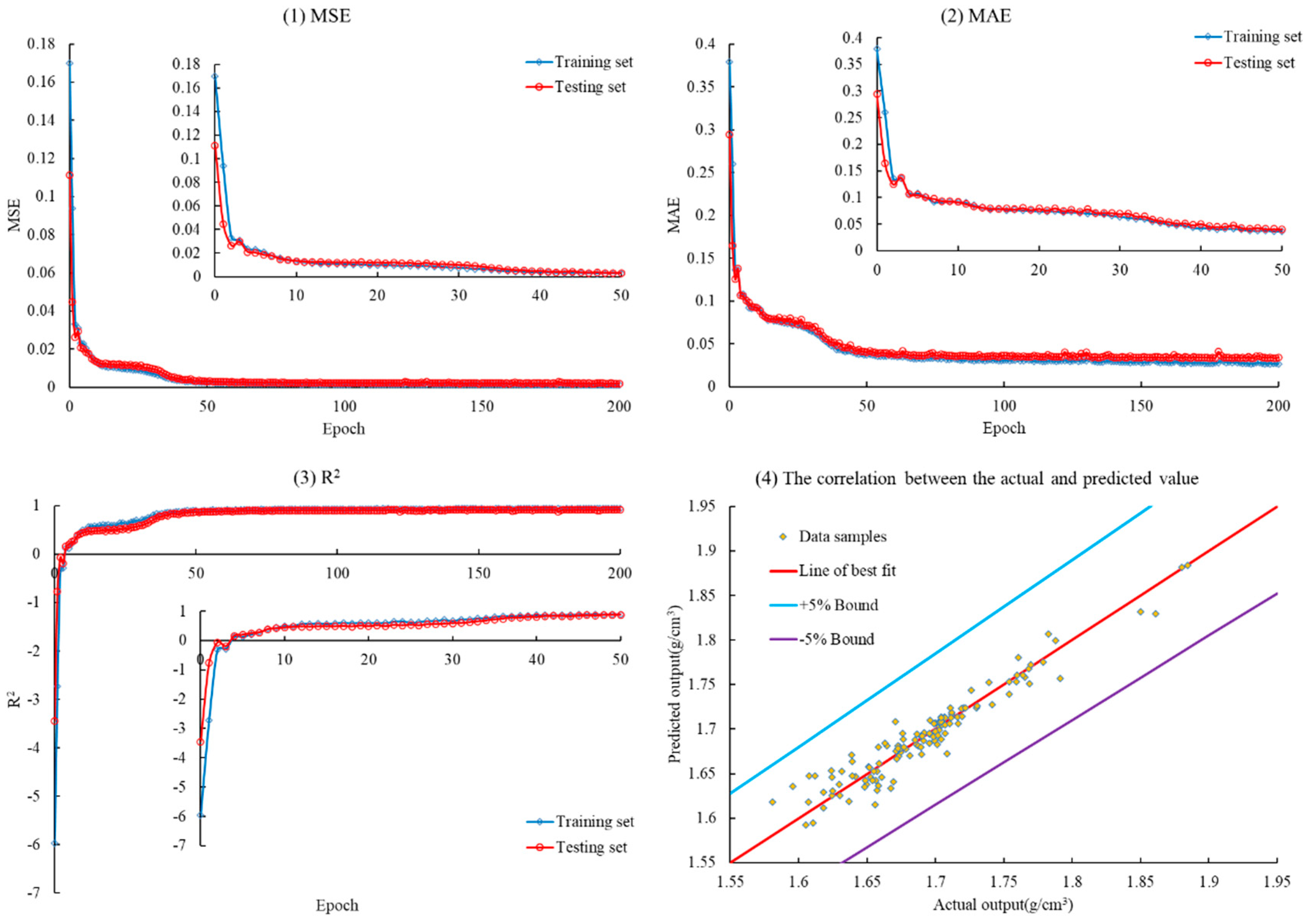
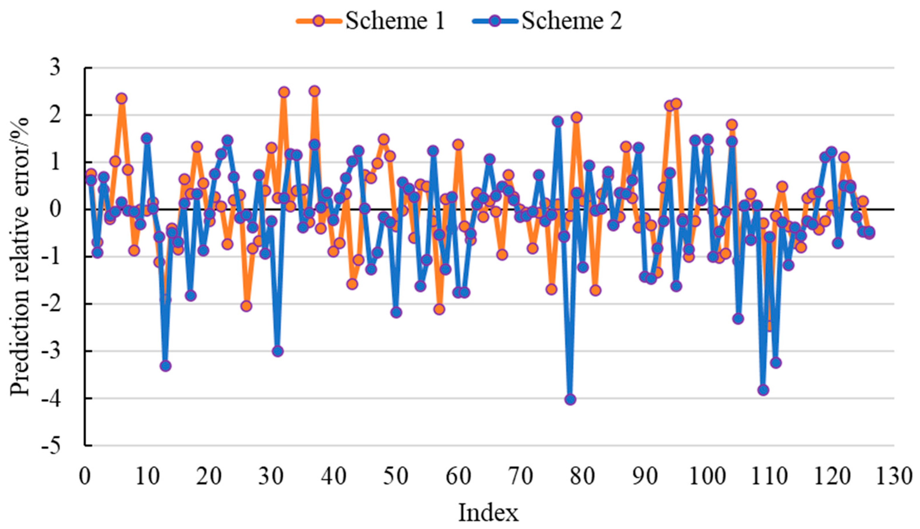
In this study, an LSTM-BP intelligent prediction model was developed to estimate formation leak-off pressure, and both Scheme 1 and Scheme 2 were employed for evaluation. The results demonstrated a significant disparity in the performance of the three evaluation metrics between the Scheme 1 and Scheme 2 models throughout the training process. Notably, the Scheme 1 model exhibited commendable performance on both the training and testing sets, whereas the Scheme 2 model displayed inadequate performance. The Scheme 1 model achieved a remarkable reduction of 992.393% and 240.674% in MSE and MAE on the testing set, respectively, in comparison to the Scheme 2 model. Furthermore, it achieved a notable increase of 66.920% in R². The Scheme 1 model demonstrated a relative error range of (−2.467%, 2.510%) and (−6.141%, 5.201%) on the testing set, confirming the high prediction accuracy of the LSTM-BP model developed in this study. Moreover, incorporating formation density as an input variable, despite lacking a direct singular correlation with leak-off pressure, did not diminish the predictive accuracy of the model. In fact, it contributed to a narrower range of relative errors.

(2)

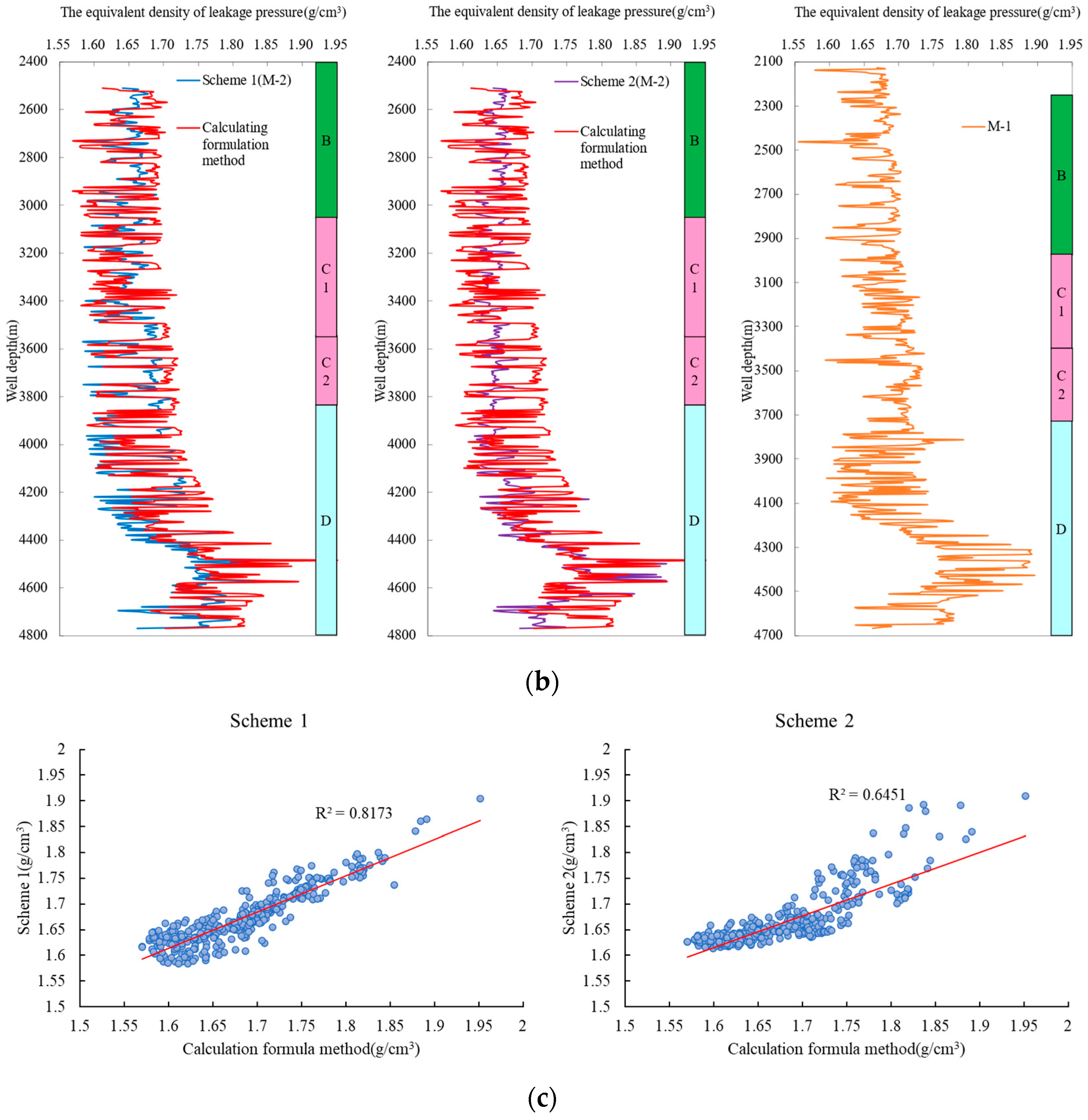
The LSTM-BP models, trained using Scheme 1 and Scheme 2, were employed to predict the formation leak-off pressure in the adjacent M-2 well. The outcomes demonstrated that the predicted values from both model schemes displayed comparable overall trends. Nevertheless, the majority of predicted outcomes from the Scheme 2 model fell within the prediction range of the Scheme 1 model, implying that the Scheme 1 model exhibited greater volatility in its predictions. Additionally, it was observed that the predicted outcomes of the Scheme 1 model closely aligned with the results derived from the formula method, whereas the Scheme 2 model exhibited noticeably inferior performance compared to the Scheme 1 model.

(3)

The models were trained using the BP and random forest algorithms based on Scheme 1 and Scheme 2. The findings revealed that, irrespective of BP or random forest, the Scheme 1 models outperformed the Scheme 2 models on the testing set. These results suggest the generalizability of the conclusions drawn in this study to other algorithms. Additionally, it was noted that both the BP and random forest models exhibited inferior performance compared to the LSTM-BP model developed in this study, highlighting the superiority of the LSTM-BP model.

(4)

The prevention of wellbore losses poses a challenging problem in the field of oil and gas exploration and development. Wellbore losses involve intricate mechanisms, and controlling them requires consideration of multiple factors. Precisely predicting formation leak-off pressure plays a crucial role in effective control measures. The development of the LSTM-BP intelligent prediction model for formation leak-off pressure, which incorporates physical data and is driven by dual factors, represents a valuable contribution to the study of formation leak-off pressure and serves to advance the progress of intelligent drilling technology. Nevertheless, this study possesses certain deficiencies and constraints. For instance, the model’s input layer solely incorporates well logging data. Subsequently, the inclusion of rock mechanical parameters like Young’s modulus and Poisson’s ratio, along with engineering logs such as drilling speed and pump pressure, into the input layer variables could be contemplated.

References

1. Arshad, U.; Jain, B.; Ramzan, M.; Alward, W.; Diaz, L.; Hasan, I.; Aliyev, A.; Riji, C. Engineered solution to reduce the impact of lost circulation during drilling and cementing in Rumaila Field. In Proceedings of the International Petroleum Technology Conference, Doha, Qatar, 6 December 2015. [Google Scholar]
2. Mehrabian, A.; Jamison, D.E.; Teodorescu, G. Geomechanics of Lost-Circulation Events and Wellbore-Strengthening Operations. SPE J. 2015, 20, 1305–1316. [Google Scholar] [CrossRef]
3. Sun, J.S.; Bai, Y.R.; Cheng, R.C.; Lyu, K.H.; Liu, F.; Feng, J.; Lei, S.F.; Zhang, J.; Hao, H.J. Research progress and prospect of plugging technologies for fractured formation with severe lost circulation. Pet. Explor. Dev. 2021, 48, 732–743. [Google Scholar] [CrossRef]
4. Kang, Y.L.; Xu, C.Y.; You, L.J.; Yu, H.F.; Zhang, D.J. Temporary sealing technology to control formation damage induced by drill-in fluid loss in fractured tight gas reservoir. J. Nat. Gas Sci. Eng. 2014, 20, 67–73. [Google Scholar] [CrossRef]
5. Zhai, X.P.; Chen, H.; Lou, Y.S.; Wu, H.M. Prediction and control model of shale induced fracture leakage pressure. J. Pet. Sci. Eng. 2021, 198, 108186. [Google Scholar] [CrossRef]
6. Morita, N.; Black, A.D.; Guh, G.F. Theory of lost circulation pressure. In Proceedings of the SPE Annual Technical Conference and Exhibition, New Orleans, Louisiana, 23 September 1990. [Google Scholar]
7. Lavrov, A.; Tronvoll, J. Modeling mud loss in fractured formation. In Proceedings of the Abu Dhabi International Conference and Exhibition, Abu Dhabi, United Arab Emirates, 10 October 2004. [Google Scholar]
8. Majidi, R.; Miska, S.Z.; Yu, M.; Thompson, L.G.; Zhang, J. Quantitative Analysis of Mud Losses in Naturally Fractured Reservoirs: The Effect of Rheology. SPE Drill. Complet. 2010, 25, 509–517. [Google Scholar] [CrossRef]
9. Lei, Q.; Xiong, W.; Yuan, J.; Cui, Y.; Wu, Y.S. Analysis of stress sensitivity and its influence on oil production from tight reservoirs. In Proceedings of the Eastern Regional Meeting, Lexington, KY, USA, 17 October 2007. [Google Scholar]
10. Lan, H.T.; Moore, I.D. New design equation for maximum allowable mud pressure in sand during horizontal Directional drilling. Tunn. Undergr. Space Technol. 2022, 126, 104543. [Google Scholar] [CrossRef]
11. Yang, M.; Yang, L.C.; Wang, T.; Chen, Y.H.; Yang, C.; Li, L.X. Estimating formation leakage pressure using a coupled model of circulating temperature-pressure in an eccentric annulus. J. Pet. Sci. Eng. 2020, 189, 106918. [Google Scholar] [CrossRef]
12. Aadnoy, B.S.; Belayneh, M. Elasto-plastic fracturing model for wellbore stability using non-penetrating fluids. J. Pet. Sci. Eng. 2004, 45, 179–192. [Google Scholar] [CrossRef]
13. Feng, Y.C.; Gray, K.E. Modeling Lost Circulation Through Drilling-Induced Fractures. SPE J. 2018, 23, 205–223. [Google Scholar] [CrossRef]
14. Wang, R.; Chen, G.; Liu, Y. A Dynamic Model of Machine Learning and Deep Learning in Shield Tunneling Parameters Prediction. In Proceedings of the 17th East Asian-Pacific Conference on Structural Engineering and Construction, 2022: EASEC-17, Singapore, 27–30 June 2022; Springer Nature Singapore: Singapore, 2023; pp. 1241–1254. [Google Scholar]
15. Chen, G.; Li, Q.Y.; Li, D.Q.; Wu, Z.Y.; Liu, Y. Main frequency band of blast vibration signal based on wavelet packet transform. Appl. Math. Model. 2019, 74, 569–585. [Google Scholar] [CrossRef]
16. Kokkinos, N.C.; Nkagbu, D.C.; Marmanis, D.; Dermentzis, K.; Maliaris, G. Evolution of Unconventional Hydrocarbons: Past, Present, Future and Environmental FootPrint. J. Eng. Sci. Technol. Rev. 2022, 15, 15–24. [Google Scholar] [CrossRef]
17. Krishna, S.; Ridha, S.; Vasant, P.; Ilyas, S.U.; Sophian, A. Conventional and intelligent models for detection and prediction of fluid loss events during drilling operations: A comprehensive review. J. Pet. Sci. Eng. 2020, 195, 107818. [Google Scholar] [CrossRef]
18. Sabah, M.; Talebkeikhah, M.; Agin, F.; Talebkeikhah, F.; Hasheminasab, E. Application of decision tree, artificial neural networks, and adaptive neuro-fuzzy inference system on predicting lost circulation: A case study from Marun oil field. J. Pet. Sci. Eng. 2019, 177, 236–249. [Google Scholar] [CrossRef]
19. Geng, Z.; Wang, H.Q.; Fan, M.; Lu, Y.H.; Nie, Z.; Ding, Y.H.; Chen, M. Predicting seismic-based risk of lost circulation using machine learning. J. Pet. Sci. Eng. 2019, 176, 679–688. [Google Scholar] [CrossRef]
20. Pang, H.W.; Meng, H.; Wang, H.Q.; Fan, Y.D.; Nie, Z.; Jin, Y. Lost circulation prediction based on machine learning. J. Pet. Sci. Eng. 2022, 208, 109364. [Google Scholar] [CrossRef]
21. Li, Z.; Chen, M.; Jin, Y.; Lu, Y.; Wang, H.; Geng, Z.; Wei, S. Study on intelligent prediction for risk level of lost circulation while drilling based on machine learning. In Proceedings of the 52nd U.S. Rock Mechanics/Geomechanics Symposium, Seattle, WA, USA, 17 June 2018. [Google Scholar]
22. Jahanbakhshi, R.; Keshavarzi, R.; Jalili, S. Artificial neural network-based prediction and geomechanical analysis of lost circulation in naturally fractured reservoirs: A case study. Eur. J. Environ. Civ. Eng. 2014, 18, 320–335. [Google Scholar] [CrossRef]
23. Hou, X.X.; Yang, J.; Yin, Q.S.; Liu, H.; Chen, H.; Zheng, J.; Wang, J.; Cao, B.; Zhao, X.; Hao, M.; et al. Lost circulation prediction in South China Sea using machine learning and big data technology. In Proceedings of the Offshore Technology Conference, Houston, TX, USA, 4 May 2020. [Google Scholar]
24. Unrau, S.; Torrione, P. Adaptive real-time machine learning-based alarm system for influx and loss detection. In Proceedings of the SPE Annual Technical Conference and Exhibition, San Antonio, TX, USA, 9 October 2017. [Google Scholar]
25. Andia, P.; Sant, R.V.; Whiteley, N. A comprehensive real-time data analysis tool for fluid gains and losses. In Proceedings of the IADC/SPE Drilling Conference and Exhibition, Fort Worth, TX, USA, 6 March 2018. [Google Scholar]
26. Li, C.; Wang, Z.R.; Rao, M.Y.; Belkin, D.; Song, W.H.; Jiang, H.; Yan, P.; Li, Y.N.; Lin, P.; Hu, M.; et al. Long short-term memory networks in memristor crossbar arrays. Nat. Mach. Intell. 2019, 1, 49–57. [Google Scholar] [CrossRef]
27. Graves, A.; Jaitly, N. Towards end-to-end speech recognition with recurrent neural networks. In Proceedings of the 31st International Conference on International Conference on Machine Learning, Beijing, China, 21–26 June 2014; JMLR.org: Beijing, China, 2014; Volume 32, pp. 1764–1772. [Google Scholar]
28. Cortez, B.; Carrera, B.; Kim, Y.J.; Jung, J.Y. An architecture for emergency event prediction using LSTM recurrent neural networks. Expert Syst. Appl. 2018, 97, 315–324. [Google Scholar] [CrossRef]
29. Habler, E.; Shabtai, A. Using LSTM encoder-decoder algorithm for detecting anomalous ADS-B messages. Comput. Secur. 2018, 78, 155–173. [Google Scholar] [CrossRef]
30. Graves, A.; Schmidhuber, J. Framewise phoneme classification with bidirectional LSTM and other neural network architectures. Neural Netw. 2005, 18, 602–610. [Google Scholar] [CrossRef]
31. Cortes, C.; Vapnik, V. Support-vector networks. Mach. Learn. 1995, 20, 273–297. [Google Scholar] [CrossRef]
32. Ma, T.S.; Zhang, Y.; Qiu, Y.; Liu, Y.; Li, Z.L. Effect of parameter correlation on risk analysis of wellbore instability in deep igneous formations. J. Pet. Sci. Eng. 2022, 208, 109521. [Google Scholar] [CrossRef]
33. Zhao, G.; Ding, W.L.; Tian, J.; Liu, J.S.; Gu, Y.; Shi, S.Y.; Wang, R.Y.; Sun, N. Spearman rank correlations analysis of the elemental, mineral concentrations, and mechanical parameters of the Lower Cambrian Niutitang shale: A case study in the Fenggang block, Northeast Guizhou Province, South China. J. Pet. Sci. Eng. 2022, 208, 109550. [Google Scholar] [CrossRef]
Figure 1. Establishment process of LSTM-BP leakage pressure intelligent prediction model.
Applsci 13 10147 g001
Figure 2. LSTM basic network structure diagram.
Applsci 13 10147 g002
Figure 3. BP neural network algorithm diagram.
Applsci 13 10147 g003
Figure 4. Stratigraphic comparison of the M-1 well and M-2 well.
Applsci 13 10147 g004
Figure 5. M-1 well input layer learning sample data violin diagram.
Applsci 13 10147 g005
Figure 6. Vertical profile of formation leakage pressure in Well M-1.
Applsci 13 10147 g006
Figure 7. M-1 well training sample data correlation heat map (Spearman).
Applsci 13 10147 g007
Figure 8. The schematic diagram of the LSTM-BP leakage pressure intelligent prediction model.
Applsci 13 10147 g008
Figure 9. Model training evaluation index map (Scheme 1).
Applsci 13 10147 g009
Figure 10. Model training evaluation index map (Scheme 2).
Applsci 13 10147 g010
Figure 11. The performance of the two scheme models on the test set.
Applsci 13 10147 g011
Figure 12. Comparison diagram of equivalent density of leakage pressure predicted by two schemes of the M-2 well model. (a) The layered profile of the predicted value of the formation leakage pressure of the two schemes of the model in Well M-2 is plotted. (b) The vertical profile of the whole well section of the predicted value of the formation leakage pressure of the M-2 well is plotted. (c) The cross-plot of the calculation results of the formation leakage pressure formula method of Well M-2 and the prediction results of the LSTM-BP model.
Applsci 13 10147 g012aApplsci 13 10147 g012b
Figure 13. The comparison of input layer variables between Well M-1 and Well M-2.
Applsci 13 10147 g013