Joint Location–Allocation Model for Multi-Level Maintenance Service Network in Agriculture

Abstract

The maintenance service network is always designed as a multi-level service network to provide timely maintenance service for failed machinery, and is rarely studied in agriculture. Thus, this paper focuses on a three-level maintenance service network location–allocation problem in agriculture, which contains several spare part centres, service stations, and service units. This research aims to obtain the optimal location of spare part centres and service stations while determining service vehicle allocation results for service stations, and the problem can be called a multi-level facility location and allocation problem (MLFLAP). Considering contiguity constraints and hierarchical relationships, the proposed MLFLAP is formulated as a mixed-integer linear programming (MILP) model integrating with P-region and set covering location problems to minimize total service costs, including spare part centre construction costs, service vehicle usage costs, and service mileage costs of service stations. The Benders decomposition-based solution method with several improvements is then applied to decompose the original MLFLAP into master problem and subproblems to find the optimal solutions effectively. Finally, a real-world case in China is proposed to evaluate the performance of the model and algorithm in agriculture, and sensitivity analysis is also conducted to demonstrate the impact of several parameters.

1. Introduction

Agricultural machinery, as key and general resources in agricultural production, are distributed over a wide geographical area in China [1]. Agricultural machinery is prone to failure due to high temperatures, complicated environments, and long-term agricultural operations, especially in the busy season [2,3]. To maintain stable production in agriculture, manufacturers always design a maintenance service network to supply maintenance for failed machinery [4,5].

In general, the maintenance service network is always designed as a multi-level service network in China, which contains several service facilities, e.g., a spare part centre and service station. This paper focuses on the design problem of the multi-level maintenance service network. In this research, the location of spare part centres and service stations is chosen from the potential location set while determining service vehicle allocation results, and the service relationship between two adjacent levels of service facilities is defined simultaneously, which can also be described to define these service stations’ service area. In summary, the problem considered in this research can be described as a multi-level facility location–allocation problem in the maintenance service network (MLFLAP).

Numerous studies on service network design have been conducted and applied in different areas, such as supply chain networks [6,7], healthcare and emergency systems [8,9,10], maintenance service networks [11], and transportation and logistics systems [12,13]. Service paradigms in agriculture bring new issues and motivate new research in the design of maintenance service networks. First, in agriculture, there is no cross-level service in the multi-level maintenance service network. That is, spare part centres are built to supply spare parts to service stations, and service stations are in charge of maintenance service for failed machinery. Thus, spare part centres cannot supply maintenance services for failed machinery directly, which is different from other service networks. In addition, different from discrete demand points in previous studies, maintenance demands in agriculture are spread across a wide geographical area. Thus, manufacturers always cluster some agricultural production areas into several service units, and maintenance demands in service units are calculated based on all failed machinery in these production areas. All service demands in the same service unit can be served by one service station. The region-based service region districting problem is a special problem in agricultural maintenance. Lastly, an adjacent production area always means a similar climate and crop-ripening time, so service units in connected areas allocated to the same service station can improve service efficiency. Contiguity constraints should be considered in this research to ensure that service units in a service region and service district are contiguous.

Thus, this paper considers the location–allocation problem in the multi-level maintenance service network, and this research aims to develop a practical solution approach to determine the location of spare part centres and service stations while determining the allocation results of service vehicles.

The contributions of this research are threefold. First, in agriculture, service stations and spare part centres need to be located considering hierarchical relationships while determining the service area of these service facilities. A defined number of service vehicles is expected to be allocated to these selected service stations to provide maintenance service for failed machinery simultaneously. Thus, a multi-level facility location–allocation problem (MLFLAP) in agriculture is proposed in this paper. Second, an MILP-based solution model is formulated for minimal service costs. Contiguity criteria are introduced to ensure that the service region served by one service station is contiguous, and multi-level constraints are applied to prohibit cross-level service. Lastly, a Benders decomposition approach with several improvements is developed to address the large-scale cases in reality efficiently, and sensitivity analysis is conducted for decision making in practical application.

2. Literature Review

Facility location–allocation problems (FLAPs) have been a research focus for several years and are applied to determine the location of service facilities and the allocation of service resources [14,15]. FLAPs have been applied in different areas, including emergency service systems [16], supply chain networks [17], transportation and logistics systems [18], urban health and services systems [19], and maintenance service networks [20].

In classical single-level FLAPs, the location of service facilities is selected and the allocation of service resources is also defined. However, there always exist multi-level facilities in service networks, and multi-level facility location–allocation problems (MLFAPs), as a subclass of FLAPs, have attracted more attention in the last two decades [15,21]. For example, Doyen et al. [22] concentrated on the two-echelon humanitarian relief logistics system and developed a Lagrangian relaxation-based heuristic algorithm to determine the location of pre- and post-disaster rescue centres. Wu and Chu et al. [23] conducted research to determine the location of plants and warehouses in reality and combined the Lagrangian relaxation method and simulated annealing algorithm to obtain minimal transportation and production costs. Shu and Wu et al. [24] considered the location problem of warehouses and retailers in a two-echelon supply chain network and developed a novel cutting-plane approach to solve the real case with moderate size. Shavarani et al. [25] focused on the facility location problem in multi-level delivery systems with retailers, refuel stations, and warehouses, and developed a novel solution method to minimize transportation costs considering demands uncertainty and M/G/K queueing system. Abbassi et al. [26] considered a multi-objective optimization model to determine the location of intermediate healthcare facilities and two heuristic algorithms, including particle swarm optimization and a non-dominated sorting genetic algorithm, were designed to solve several case studies in healthcare supply chain logistics.

As for mathematical models for FLAPs, they are always formulated as mixed-integer program (MIP) models. For example, Zamani et al. [27] developed a mixed-integer programming model to solve congested facility location problems considering machine failures. Muffak et al. [28] considered the fixed and dynamic demand and developed a mixed-integer linear programming model to determine the location of public facilities. Govindan et al. [29] focused on facility location problems in food supply chain networks and formulated a multi-objective model to determine the number and location of service facilities. Talaei et al. [30] constructed an MIP-based optimization model to determine the location of collection/inspection centres and minimize the total costs in a closed-loop green supply chain system. Ghasemi et al. [16] developed a multi-objective optimization model to minimize total allocation costs while minimizing the total amount of relief suppliers. Tirkolaee et al. [31] considered the service facility location problem in urban service systems and formulated an MILP for minimal costs based on the robust optimization approach.

Solution approaches in FLAPs can be classified into two groups: exact approaches and heuristic algorithms [32,33]. As for exact approaches, Sonmez et al. [34] designed a decomposition-based solution approach to obtain a near-optimal location plan and compared it with another exact method to demonstrate the performance of the developed approach. Fischetti et al. [35] combined the Benders decomposition method and commercial solver with the brand and cut method to obtain the best service facility location, and computational results were presented to show the method’s efficiency compared with exact methods and heuristic algorithms. Irawan et al. [36] combined the integer linear programming method and aggregation approach to obtain the optimal location of distribution centres. Several experiments were conducted to demonstrate the efficiency of the developed method compared with other exact approaches. Han and Zhang et al. [37] developed a Benders decomposition-based exact approach to determine the location of the service facility and service region in each stage. Chandra et al. [38] developed an exact algorithm integrating with the convexification strategy and branch and cut method for solving larger cases in the real world. Christensen et al. [39] focused on the capacitated facility location problem. Lagrangean relaxation was applied for the nonlinear objective function, and the branch and bounded method was then introduced to obtain an optimal location plan with a lower bounding scheme. Qi et al. [40] proposed a brand-and-brunch-based solution method, and two valid inequalities were introduced with an approximation algorithm to obtain the optimal results.

Considering heuristic algorithms for FLAPs, Meng et al. [41] developed a hybrid genetic algorithm integrating with a logarithmic-quadratic proximal prediction–correction method to obtain the optimal location of retailers in a decentralized supply chain system. Jolia et al. [42] designed an improved particle swarm optimization method to solve the multi-objective in dynamic facility location problem. Rahmaniani et al. [43] proposed a MIP-based optimization model, and an improved firefly algorithm-based heuristic approach was designed to solve a larger case with more than 100 nodes and 600 candidates. Halper et al. [44] concentrated on the mobile facility location problem and developed two local search neighbourhood algorithms to solve two subproblems in reality. Al-Rabiaah et al. [45] developed a heuristic solution approach integrating the greedy search and maximum coverage approach to determine the location and allocation of drone launching centres. Kang [46] considered these NP-hard problem and proposed a heuristic solution method based on maximum flow to find the optimal location. In addition, other heuristic algorithms were also applied to obtain the optimal location of a service facility in the service network, e.g., the simulated annealing algorithm [47], the kernel search heuristic algorithm [48], the tabu search method [49], and the greedy search heuristic approach [50].

In all, although several studies have been conducted on FLAPs, few studies exist on multi-level FLDPs in maintenance service networks, especially in agriculture. In addition, unlike in traditional studies, maintenance demands in connected areas are always clustered as a service unit in agriculture, and few studies consider facility location problems based on service district. Therefore, it is urgent to develop a more comprehensive solution framework considering contiguity criteria and multi-level constraints in maintenance service networks in agriculture.

3. Problem Description and Model Formulation

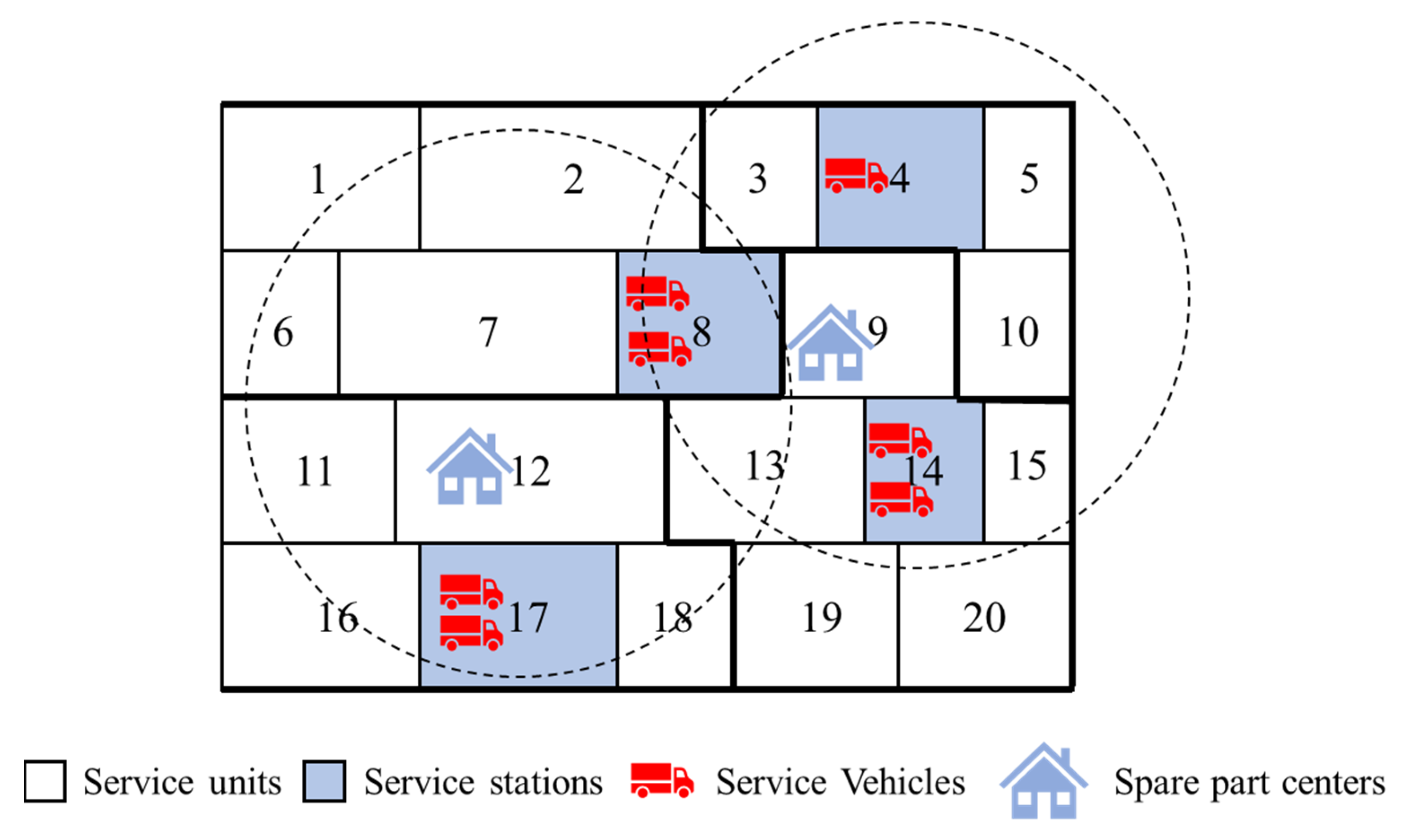
3.1. Problem Description

To supply timely maintenance for failed machinery in the busy farming seasons, manufacturers always construct a multi-layer maintenance service network. There exist three layers in the service network, which include spare part centres, service stations, and service units. Service units are a set of connected production areas including agricultural machinery, just like a county in China, and a connected service area always means a similar climate and ripening time, which represents maintenance demands. Service stations with several service vehicles are built by manufacturers to supply maintenance for the demand for service units.

Thus, the multi-layer facility location–allocation problem (MLFLAP) can be described as follows. There are n service units with defined maintenance demands in agriculture. In order to supply maintenance, l service stations are selected from the potential location set of service stations to supply maintenance service, and m service vehicles with defined service capacity are allocated to the selected service stations. In addition, several spare part centres are built by the manufacturer to supply spare parts for service stations.

Assuming that there are 20 service units, four service stations are selected to supply service for these service units, and nine service vehicles are allocated to the selected service stations. In Figure 1, service stations are located in service units 4, 8, 14, and 17, and the service units served by each service station are distinguished by bold lines. As for service station 4, there exists one service vehicle that can provide maintenance service for four service units, e.g., 3, 4, 5, and 10. As for service station 17, two service vehicles are allocated to this service station, and five service units, such as 11, 12, 16, 17, and 18, are served by service station 17. In addition, an indefinite number of spare part centres are built by the manufacturer to supply spare parts for service stations, which are served by the nearest spare part centres. As shown in Figure 1, in order to supply spare parts for service stations, two spare part centres are selected in service units 12 and 9, and the maximal distribution distance for these spare part centres is shown with black dotted lines. Thus, the spare part centre in 9 can supply spare parts for service stations 4, 8, and 14, while the spare part centre in 12 can supply spare parts for service stations 8 and 17.

Thus, the proposed MLFLAP can be divided into several subproblems: (1) Service station location and allocation problem in agriculture, which is to decide the location of service stations while allocating service vehicles to these stations. (2) Spare part centre location problem, which is to determine the location of spare part centres. (3) Service unit allocation problem, which is to assign these service units to selected service stations. The objective of the proposed MLFLAP is to minimize total costs, which include total service mileage costs from service stations to service units, total usage costs of service vehicles, and total construction costs for spare part centres.

Several assumptions are presented in this research:

(1) The maintenance requirement in service units is known.

(2) One service unit can only be served by one service station.

(3) Several service units served by one service station are continuous.

(4) There is a defined service capacity for service vehicles, and there exists a maximal distribution distance for spare part centres to service stations.

3.2. Nomenclature

As for the proposed MLFLAP, two subproblems, such as the service station location and allocation problem and the spare part centre location problem, are considered in this paper, which can be seen as a joint optimization problem integrating with the P-region problem and set covering location problems. Thus, this paper formulates an MILP-based solution model. Several parameters and variables are defined first:

(1) Sets:

I	Set of service units indexed by i or i′;
J	Set of the potential location of service stations indexed by j,$J\subseteq I$;
K	Set of the potential location of spare part centres indexed by k,$K\subseteq I$;
A	Set of adjacent service unit pairs.

(2) Parameters:

n	The number of service units;
m	The number of service vehicles;
l	The number of chosen service stations;
$d_i^j$	Distance from the potential location of service station j to service units i;
$D_j^k$	Distance between the potential location of service station j and potential location of spare part centre k;
c1	The construction costs per spare part centre;
c2	The usage costs per service vehicle;
c3	The service mileage costs for service stations to service units per kilometre;
$r_i$	Maintenance demand requirements in each service unit i;
D1max	Maximal service distance for service stations to service units;
D2max	Maximal service distance for spare part centres;
C	The maximal service capacity per service vehicle;
M	A constant more than the number of service units.

(3) Variables:

xk	If the spare part centre is set in location k, the value is 1; otherwise, it is 0;
$y_j$	If the service station is set in location j, the value is 1; otherwise, it is 0;
$z_i^j$	If service unit i is served by the potential location of service station j, the value is 1; otherwise, it is 0;
$v_j$	The number of service vehicles allocated to potential locations j;
$u_j^k$	If the potential location of service station j can be served by the potential location of spare part centre k, the value is 1; otherwise, it is 0;
$w_{ii\prime }^j$	The contiguity evaluation for optimal location–allocation results. The variable for contiguity evaluation to indicate the imaginary flow from service unit i to service unit i′, which is served by service station j.

3.3. Mathematical Model

The MILP-based optimization model P₀ is used to obtain the minimal service costs, which is shown as follows:

$${\mathbf{P}}_{0}Minf={\displaystyle \sum _k{c}_1\times x_k+{\displaystyle \sum _j{c}_2\times v_j+{\displaystyle \sum _j{\displaystyle \sum _{i}2\times c_3\times z_i^j}}}}\times d_i^j\times r_i$$

(1)

The objective function (1) aims to obtain minimal service costs, which include total construction costs for spare part centres, total usage costs for service vehicles, and total service mileage costs for service stations:

s. t.

$$u_j^k\le x_k,\forall j,\forall k$$

(2)

$${\displaystyle \sum _k{u}_j^k}\ge y_j,\forall j,\forall k$$

(3)

$$u_j^k\times D_j^k\le D{2}_{\max },\forall j,\forall k$$

(4)

$${\displaystyle \sum _j{v}_j}\le m$$

(5)

$$C\times v_j\ge {\displaystyle \sum _i{z}_i^j}\times r_i,\forall j$$

(6)

$${\displaystyle \sum _j{y}_j}=l$$

(7)

$${\displaystyle \sum _j{z}_i^j=1,}\forall i$$

(8)

$${\displaystyle \sum _i{z}_i^j=y_j,}\forall j$$

(9)

$$z_i^j\le y_j,\forall i,\forall j$$

(10)

$${\displaystyle \sum _j{\displaystyle \sum _i{z}_i^j}=n}$$

(11)

$$z_i^j\times d_i^j\le D{1}_{\max },\forall i,\forall j$$

(12)

$${\displaystyle \sum _{i\prime |(i,i\prime )\in A}{w}_{ii\prime }^j}-{\displaystyle \sum _{i\prime |(i\prime ,i)\in A}{w}_{i\prime i}^j}=z_i^j,\forall i,\forall j,i\ne j$$

(13)

$${\displaystyle \sum _{i\prime |(i,i\prime )\in A}{w}_{ii\prime }^j}\le (M-2)\times z_i^j,\forall i,\forall j,i\ne j$$

(14)

$${\displaystyle \sum _{i\prime |(i\prime ,j)\in A}{w}_{i\prime j}^j}\le (M-1)\times y_j,\forall j$$

(15)

$$w_{ii\prime }^j\ge 0,\forall i,\forall i\prime ,\forall j$$

(16)

$$v_j\ge 0,\forall j$$

(17)

$$y_j,x_k,u_j^k,z_i^j=\{0,1\},\forall i,\forall j,\forall k$$

(18)

Constraints (2) and (3) ensure that all these chosen service stations can be served by the spare part centres. Constraint (4) implies the maximal service distance for spare part centres. Constraint (5) restricts the number of service vehicles allocated to service stations, and constraint (6) ensures the service capacity of service stations. Constraint (7) defines the number of chosen service stations. Constraints (8) and (9) specify that one service unit can only be served by one service station. Constraints (10) and (11) introduce a limitation that all service units must served by the chosen service stations. Constraint (12) enforces the maximal service distance for the service station. Constraints (13)–(15) refer to Han and Zhang [37] and are extended for contiguity constraints in service regions served by service stations. Constraint (13) is applied to calculate the imaginary flow from the service unit to the chosen service stations. Constraints (14) and (15) are introduced to prohibit the imaginary flow from other service stations. Constraints (16)–(18) specify the range of decision variables.

4. Benders Decomposition Approach

4.1. MP and SP in Benders Decomposition

Considering two integer variables w and v in the proposed MLFLAPs, a variant Benders decomposition, which is called compound Benders decomposition in this paper, is introduced to decompose the original MLFLAPs into the master problem (MP) and two subproblems (SP₁ and SP₂). In MP, the location of service stations and spare part centres are determined in this paper using the decision variables x, y, z, and u. As for SP₁, decision variables v are introduced to determine the service vehicle allocation, and in SP₂, decision variables w are introduced for contiguity evaluation of service units served by one service station.

$$\begin{array}{c}MP\hspace{1em}Min{\displaystyle \sum _k{c}_1\times x_k+{\displaystyle \sum _j{\displaystyle \sum _{i}2\times c_3\times z_i^j}}}\times d_i^j\times r_i+q\hspace{1em}\\ \text{Subject} \text{to} \text{constraints}\left(2\right)\mathrm{–}\left(4\right)\left(7\right)\mathrm{–}\left(12\right) \text{and} \left(17\right)–\left(18\right).\end{array}$$

(19)

$$\begin{array}{c}S{P}_1\hspace{1em}\min {\displaystyle \sum _j{c}_2\times v_j} \\ \text{Subject} \text{to} \text{constraints}\left(5\right)–\left(6\right) \text{and} \left(17\right)\end{array}$$

(20)

$$\begin{array}{c}S{P}_2\hspace{1em}0:w\\ \text{Subject} \text{to} \text{constraints} \left(13\right)–\left(16\right)\end{array}$$

(21)

4.2. MP and SP in Benders Decomposition

As for decision variables v in SP₁, they are applied to obtain minimal service vehicle usage costs and are subject to constraints (5)–(6) and (17). Thus, the dual SP₁ for variable v is shown as DSP₁.

$${\mathbf{DSP}}_1\max m\times \alpha +{\beta }_j\times {\displaystyle \sum _i{z}_i^j}\times r_i$$

(22)

s. t.

$$C\times \alpha +{\beta }_j\le c_2$$

(23)

$$\alpha \le 0$$

(24)

$${\beta }_j\ge 0,\forall j$$

(25)

Thus, during the Benders decomposition approach, the obtained facility location results and service assignment plan will be introduced to DSP₁ to solve the DSP₁. If there is no feasible solution for DSP₁, there is no feasible solution for the original MLFLAPs, which means the number of service vehicles cannot meet all maintenance demands in the service network. If the DSP₁ is unbounded, there exist optimal solutions for original MLFLAPs, and the generated Benders feasibility cuts in (26) are added in MP. If the DSP₁ is feasible and bounded, the generated Benders optimality cuts in (27) are added in MP.

$$m\times \alpha +{\beta }_j\times {\displaystyle \sum _i{z}_i^j}\times r_i\le 0$$

(26)

$$m\times \alpha +{\beta }_j\times {\displaystyle \sum _i{z}_i^j}\times r_i\le q$$

(27)

As for SP₂, the facility location results and service assignment results obtained in MP are introduced for contiguity evaluation. If the SP₂ returns a feasible solution, the service units served by service stations are contiguous. Otherwise, it demonstrates that there exists at least one service unit which is not contiguous with other service units served by one service station. Selected locations of service stations that are not contiguous are denoted as J*. Thus, as for these service units served by these service stations in J*, at least one service unit should be removed or one new service unit should be added, which can be described as shown in constraint (28). Thus, the combinatorial Benders cuts in (28) are generated and added to MP.

$${\displaystyle \sum _{i:{\overline{y}}_i^j=0}{y}_i^j}+{\displaystyle \sum _{i:{\overline{y}}_i^j=1}(1-y_i^j})\ge 1,\forall j\in J*$$

(28)

4.3. The Framework of Benders Decomposition

Thus, the Benders decomposition approach is applied to obtain the location–allocation results in a multi-level maintenance service network. As shown in Figure 2, the detailed information of the developed solution algorithm is described as follows.

Step 1. Input initial data.

Step 2. MP is solved to obtain a feasible solution ($\overline{x},\overline{y},\overline{z},\overline{u}$), and LB (Lower Bounded) is updated.

Step 3. The obtained service station location results $\overline{y}$ and service assignments plan $\overline{z}$ are introduced to DSP₁. If the DSP₁ is infeasible, there are no results for the original problem. If the DSP₁ is unbounded, the generated Benders feasibility cuts (26) are added in MP, and a feasible solution is found to update UB (Upper Bounded). And if the DSP₁ is feasible and bounded, the generated optimality cuts (27) are added in MP, and UB is updated.

Step 4. The obtained service station location results $\overline{y}$ and service assignments plan $\overline{z}$ are introduced to SP₂. If it returns a feasible solution, service units served by service stations are contiguous. Otherwise, the generated Benders cuts (28) are added in MP.

Step 5. Calculate the difference between UB and LB, and determine if SP₂ is feasible. If SP₂ is feasible and the values of UB and LB are equal, the optimal results of MLFLAPs are obtained. Otherwise, repeat Step 2 to Step 4.

5. Case Study

In this section, a real case in East China is conducted to demonstrate the efficiency of the proposed mathematical model and solution algorithm. The real maintenance data in three provinces, e.g., Shandong, Anhui, and Jiangsu, is shown first and the optimal location–allocation plan is then obtained in the next part. Finally, several analyses are conducted to verify the application and performance of the developed mathematical model and solution approach.

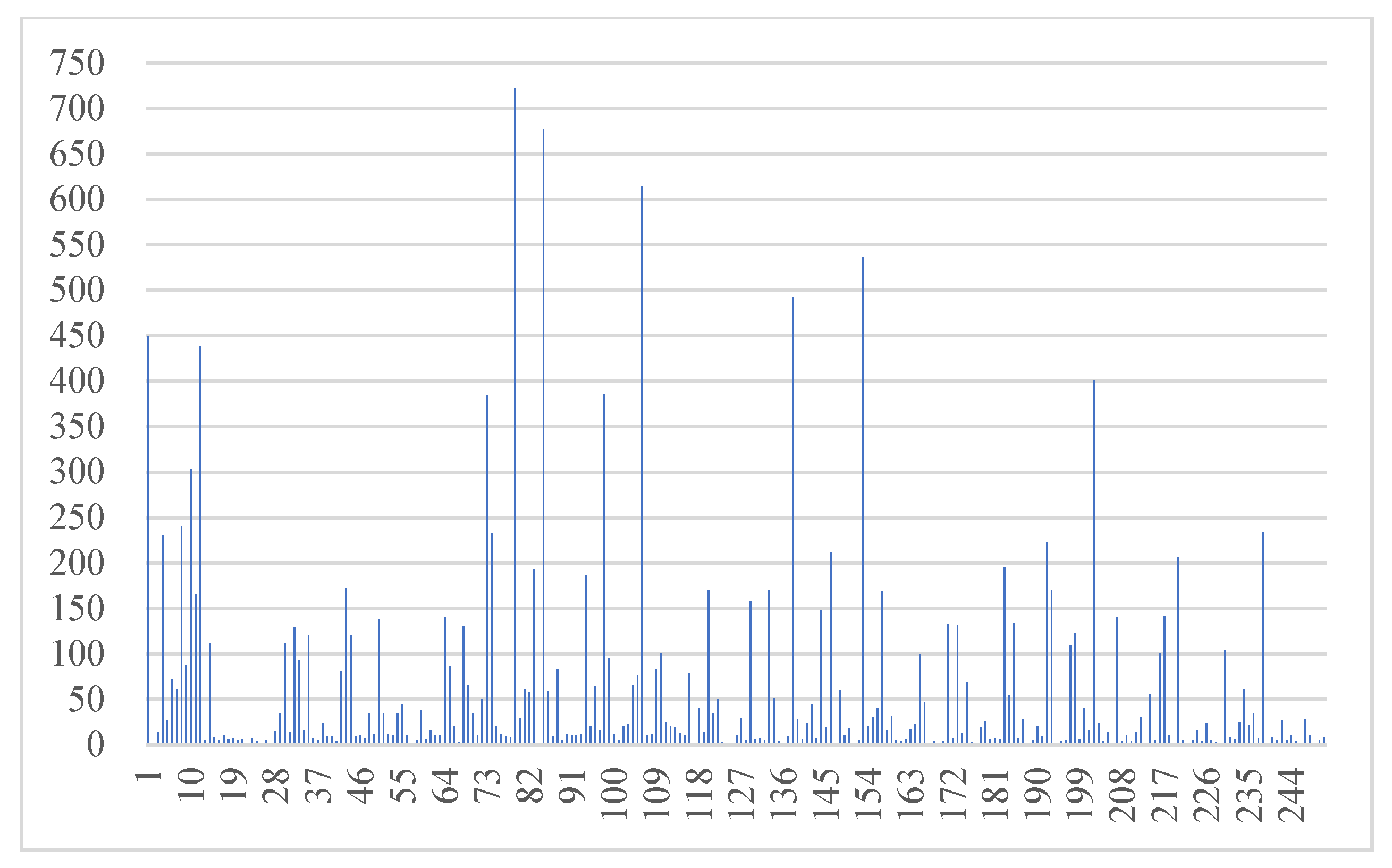
5.1. Case Description

In this part, the maintenance service network is built, including three provinces in East China, namely Shandong, Anhui, and Jiangsu, and the maintenance data are obtained from a leading agricultural machinery manufacturer in China. As shown in Figure 3, there exist 251 service units in agriculture, and maintenance demands in these service units are shown in Figure 4. The manufacturer wants to construct 25 service stations in these 251 service units. In addition, the manufacturer can provide 75 service vehicles to be allocated to these service stations. The maximal service capacity per service vehicle is 300, and the usage costs per service vehicle are CNY 800.

In order to satisfy the maintenance demands efficiently, the maximal service distance for service stations is set as 200 km. As for spare part centres, the construction costs for per spare part centre are set as CNY 10,000, and the maximal distribution distance for spare part centres is set as 360 km. In addition, the travelling distance between two service units is obtained from Baidu Map, and the service mileage costs (from service stations to service units) are set as CNY 0.5.

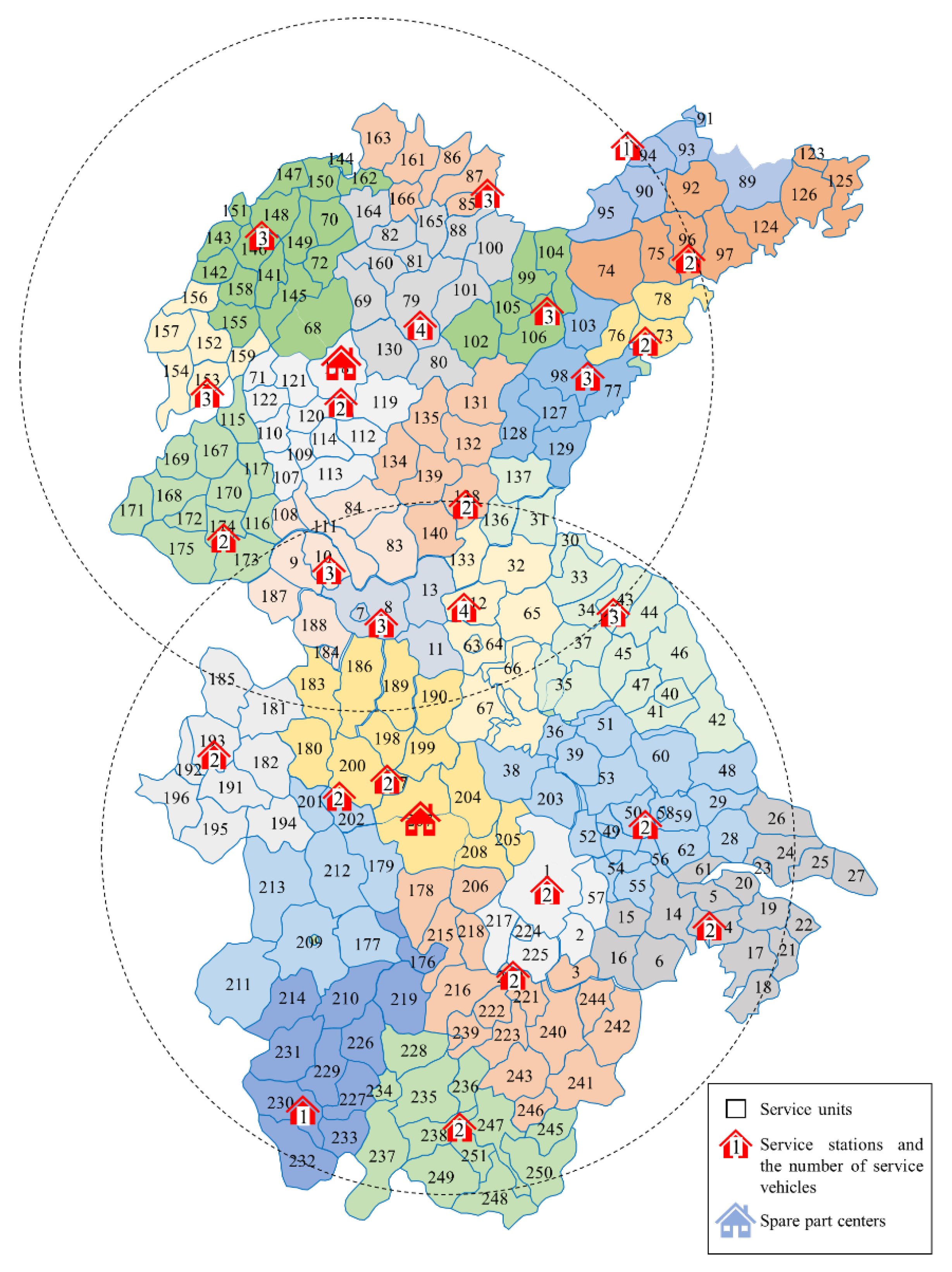
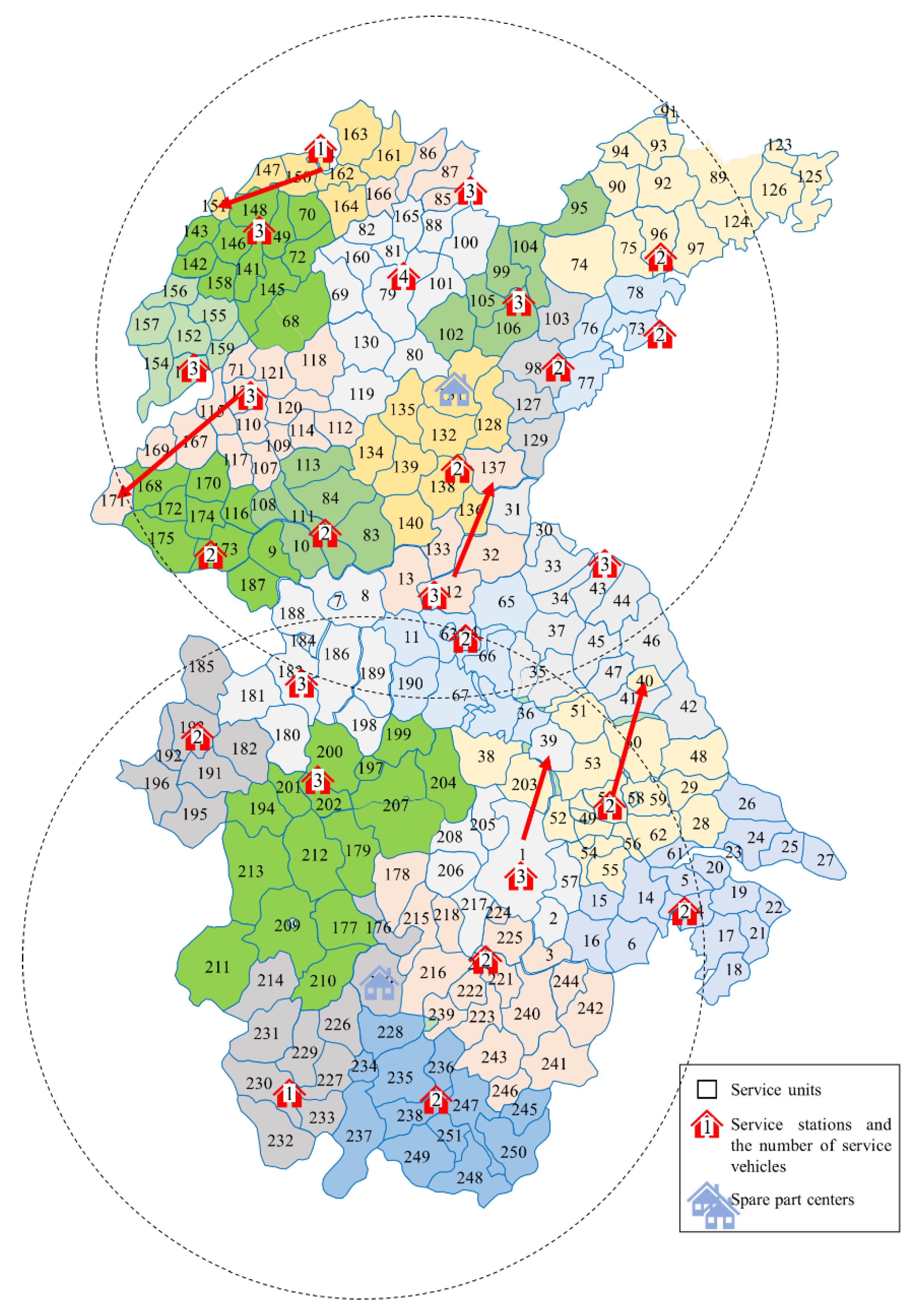
5.2. Optimal Location–Allocation Plan

In this section, the Benders decomposition solution approach is developed to solve the proposed MLFLAPs, and all computing programs are coded on a personal computer with an AMD 4.00 GHz processor.

First, the commercial solver GUROBI is introduced to solve the proposed MLFLAPs directly, but the optimal results can only be obtained after about 20 h (71,933 s) due to the massive decision variables and constraints, which may not be applicable in reality. The developed Benders decomposition approach is then applied to this problem. The optimal solutions are obtained with three iterations in 8727 s (2.4 h), and the minimal service costs in this case is 5.836 × CNY 10⁵. The location–allocation results of service stations and spare part centres are shown in

Table 1. The location allocation results in the service network.

NO.	Service Stations	Number of Vehicles	Service Units	Spare Part Centres
1	1	2	1, 2, 57, 217, 224, 225	207
2	4	2	4, 5, 6, 14, 15, 16, 17, 18, 19, 20, 21, 22, 23, 24, 25, 26, 27, 61	207
3	8	3	7, 8, 11, 13	118, 207
4	10	3	9, 10, 83, 84, 108, 111, 184, 187, 188	118, 207
5	12	4	12, 32, 63, 64, 65, 66, 67, 113	118, 207
6	43	3	30, 31, 33, 34, 35, 37, 40, 41, 42, 43, 44, 45, 46, 47, 136, 137	118, 207
7	50	2	28, 29, 36, 38, 39, 40, 48, 49, 50, 51, 52, 53, 54, 55, 56, 58, 59, 60, 62, 203	207
8	73	2	73, 76, 78	118
9	79	4	69, 79, 80, 81, 82, 88, 100, 101, 130, 160, 164, 165	118
10	85	3	85, 86, 87, 161, 163, 166	118
11	94	1	89, 90, 91, 93, 94, 95	118
12	96	2	74, 75, 92, 96, 97, 123, 124, 125, 126	118
13	98	3	77, 98, 103, 127, 128, 129	118
14	106	3	99, 102, 104, 105, 106	118
15	120	2	71, 107, 109, 110, 112, 113, 114, 18, 119, 120, 121, 122	118
16	138	2	131, 132, 134, 135, 138, 139, 140	118, 207
17	146	3	68, 70, 72, 141, 142, 143, 144, 145, 146, 147, 148, 149, 150, 151, 155, 158	118
18	153	3	152, 153, 154, 156, 157, 159	118
19	174	2	115, 116, 117, 167, 168, 169, 171, 172, 173, 174, 175	118
20	193	2	181, 182, 185, 191, 192, 193, 195, 196	207
21	197	2	180, 183, 186, 189, 190, 197, 198, 199, 200, 204, 205, 207, 208	207
22	202	2	177, 179, 194, 201, 202, 209, 211, 212, 213	207
23	220	2	3, 178, 206, 215, 216, 218, 220, 221, 222, 223, 239, 240, 241, 242, 243, 244, 246	207
24	230	1	176, 210, 214, 219, 226, 227, 229, 230, 231, 232, 233	207
25	238	2	228, 234, 235, 236, 237, 238, 245, 247, 248, 249, 250, 251	207

and Figure 5.

As shown in Figure 5, 25 service stations and two spare part centres are built in this service network. First, service stations are usually selected in these service units with a higher number of service demands, such as service units 1, 12, 79, 85, 106, 138, 153, 202, and 238. Service units served by one service station are distinguished by different colours, and all 251 of these service units are always allocated to the nearest service stations. For example, the service station in 73 provides maintenance service for three service units, e.g., 73, 76, and 78. Otherwise, the service station in 220 provides maintenance service for seventeen service units, e.g., 3, 178, 206, 215, 216, 218, 220, 221, 222, 223, 239, 240, 241, 242, 243, 244, and 246.

In addition, there are 60 service vehicles are allocated to these selected service stations based on the service demands in their service area. For example, four service vehicles are allocated to the service station in 12 with a total maintenance demand of 1168, while only one service vehicle is allocated to the service station in 94 with a total maintenance demand of 246.

As for spare part centres, two spare part centres are set in service units 118 and 207, and the service area of these two spare part centres is shown in Figure 5 with the black dotted lines. They are responsible for supplying spare parts for service stations in the top and bottom areas in Figure 5, respectively. In this case, service stations in 8, 10, 12, 43, and 138 can be served by these two spare part centres.

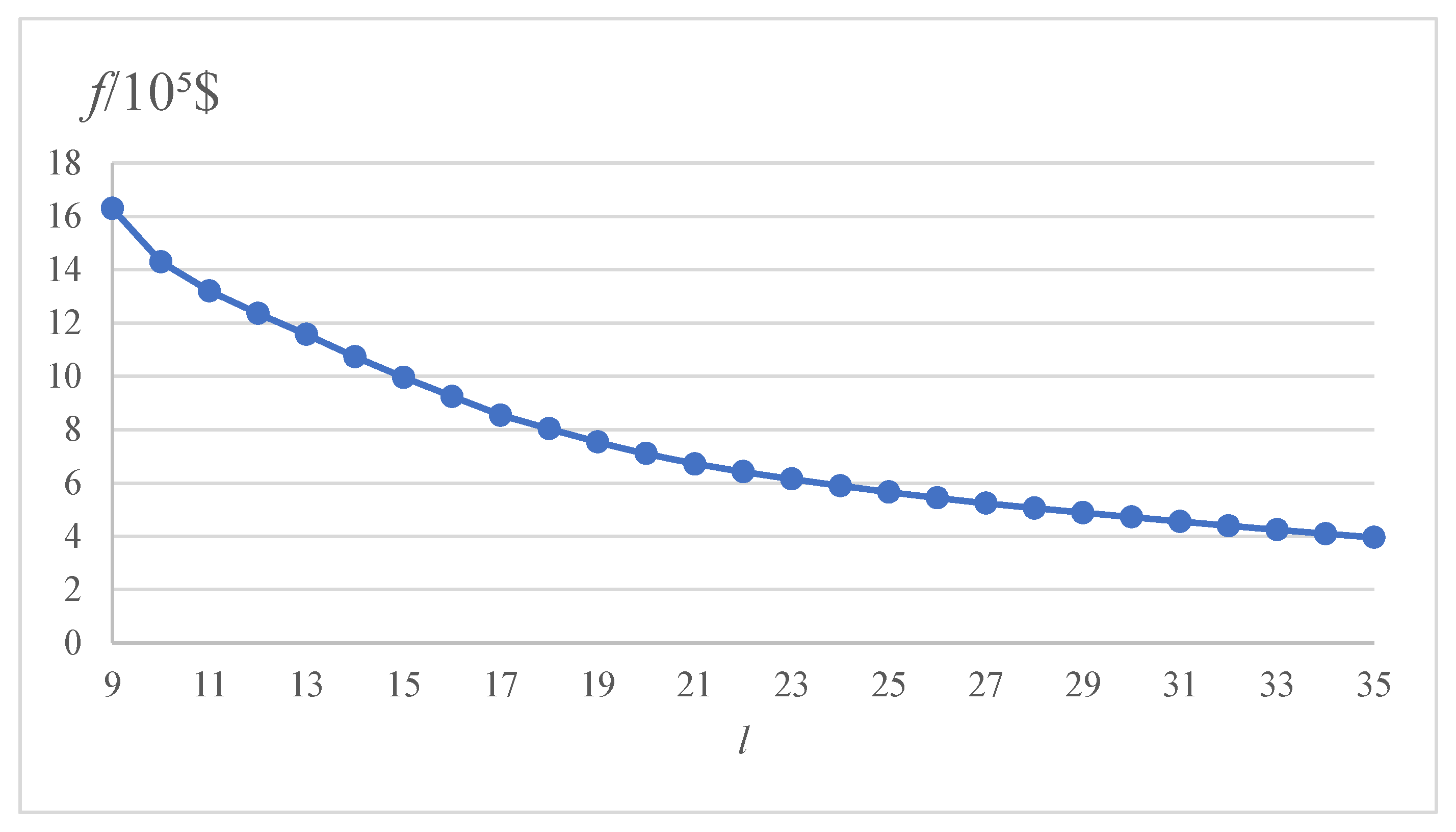
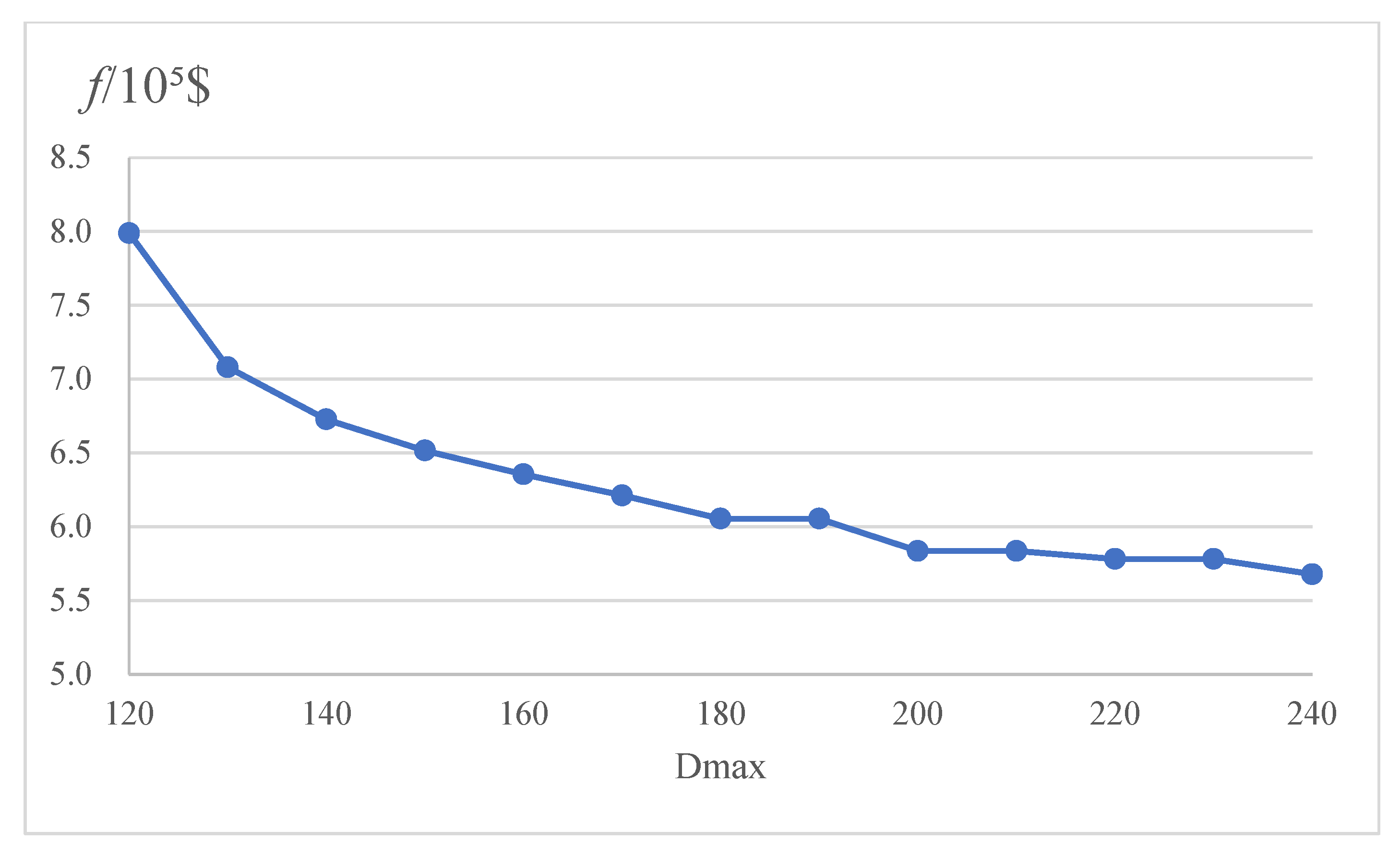
5.3. Sensitivity Analysis of Selected Parameters

In this section, sensitivity analysis is conducted to evaluate the effect of several parameters on the final results, which include the following: (a) the number of service stations, l; (b) the maximal service distance for service stations, D1_max.

First, this paper conducts a sensitivity analysis of the number of service stations, l. Several examples are conducted to find the minimum value of l, and the computational results show that there is no optimal solution when the value of l is less than 9 due to the restrictions on the number and the maximal service distance of the service vehicles. After determining the lower bounded of l, sensitivity analysis of the number of service stations l is conducted after increasing the value of l from 9. Computational results with different values of l are shown in Figure 6. Total service costs experience a downward trend as l increases from 9 to 35, and the reduction becomes smaller with the increase in the value of l. For example, total service costs reduce by 12.31% when l changes from 9 to 10, whereas total service costs reduce by 3.37% when l increases from 34 to 35. Thus, in this case, the number of service stations may be set as 20 to 30 from a comprehensive perspective.

This paper then changes the value of D1_max to examine the effect of maximal service distance of service stations on total service costs. Multi-level facility location–allocation problems without the constraints of maximal service distance are first obtained, and the total service costs are 5.678 × CNY 10⁵ with the maximal service distance of 237 km. After that, the maximal service distance for service stations is reduced from 240 km by 10 km each time, and optimal results are obtained using the proposed solution algorithm, which is shown in Figure 7. The optimal results show that the total service costs increase with the decrease in the value of D_max, and there is no optimal solution until the maximal service distance D_max is less than 120 km. Thus, manufacturers usually choose a suitable maximum service distance to ensure that they can obtain a small service cost while improving customer satisfaction. Therefore, the maximal service distance may be set as 130 km to 160 km from a comprehensive perspective.

5.4. Analysis of Contiguity Constraints

In the MIP-based optimization model, contiguity constraints (13)–(16) are introduced to ensure all service units served by one service station are geographically contiguous. Thus, to analyse the effect of the contiguity constraints in MLFLAPs, optimal solutions without constraints (13)–(16) are obtained in this section. The total service costs without contiguity constraints are 5.760 × CNY 10⁵, a 1.30% reduction compared with the costs in Section 5.2.

The location of service stations and districting results without contiguity constraints are shown in Figure 8. The service districts served by service stations 1, 50, 12, and 122, are not contiguous, and service units 39, 40, 137, and 171 are served by the corresponding service stations across other service districts. In reality, the cross-regional maintenance service shown in Figure 8 is not generally a feasible solution in agriculture, which results in a long service latency and resource waste [5]. In agriculture, the decision-maker may prefer to assign these service units to the nearest service stations, such as allocating service unit 39 to service station 50, service unit 40 to service station 43, service unit 137 to service station 138, and service unit 171 to service station 173.

In all, contiguity constraints should be considered to prohibit cross-region services and ensure a contiguous service area for managers in practical application.

5.5. The Performance of Benders Decomposition Approach

The Benders decomposition approach is analysed in this section. First, the cases in Figure 6 and Figure 7 are solved by the Gurobi solver, which cannot be obtained in less than 12 h. Especially for some cases in Figure 6 and Figure 7, the optimal solutions cannot be obtained in less than 24 h. But for the Benders decomposition approach, all optimal solutions can be obtained in 3 h.

In addition, the Gurobi and Benders decomposition solvers are applied to solve several cases with different sizes. The calculation time using different solution methods is shown in

Table 2. The performance of the Bender decomposition approach.

NO.	The Number of Service Units	The Number of Service Stations	Time_Gurobi/s	Time_Benders/s
1	50	5	21.83	25.98
2	75	8	160.20	71.5
3	100	10	522.41	174.41
4	125	12	2333.45	1277.95
5	150	15	6329.20	499.09
6	175	17	52,400.61	781.06
7	200	20	>12 h	1635.64
8	225	25	>12 h	2006.72
9	250	30	>24 h	7682.50

. As shown in Table 2, the calculation time of the Gurobi solver is shorter than that of the Benders decomposition algorithm only when the number of service units is less than 50. When the number of service units is greater than 50, the solution time using the commercial Gurobi solver will be much greater than that of the Benders decomposition algorithm. Even when the number of service units exceeds 200, the Benders decomposition algorithm can still obtain the optimal solution in 3 h, while the optimal solution cannot be obtained within 24 h using the commercial Gurobi solver.

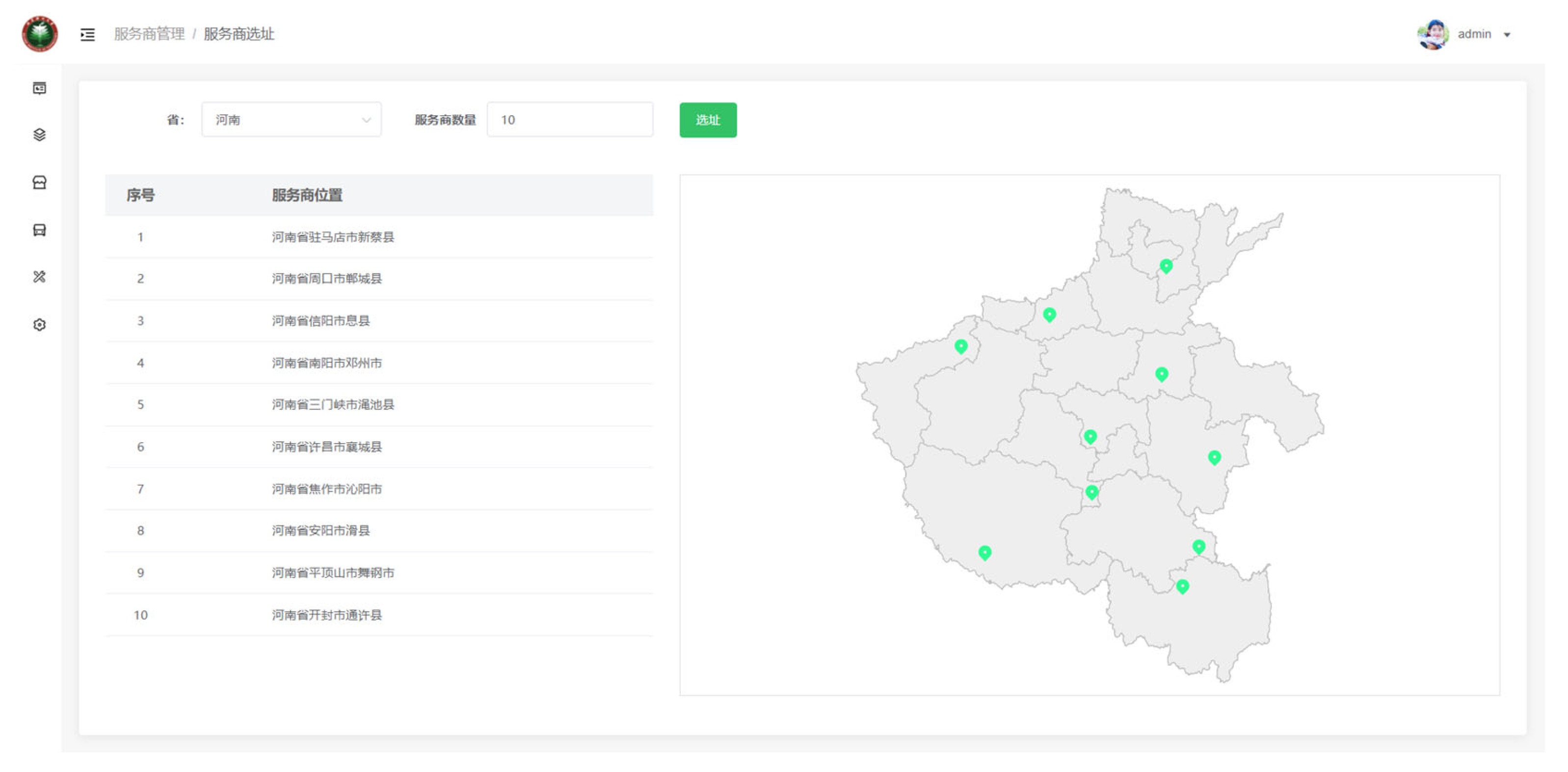
5.6. Practical Application in Agriculture

In practical application, agricultural machinery always requires the construction of a multi-level maintenance service network including spare part centres and service stations to supply spare parts and provide maintenance service in a broad geographic agricultural operation area. For example, a famous agricultural machinery manufacturer in China has constructed several spare part centres in Harbin, Tianjin, Fuyang, and so on, and the manufacturer has built more than 300 service stations in China.

Thus, the proposed MIP-based optimization model and solution approach can be applied to solve the multi-level facilities location and service resource allocation problem, which can reduce service costs effectively and improve maintenance service.

Furthermore, agricultural maintenance service network software is developed to determine the location of service stations and spare part centres in China. As shown in Figure 9, the practical application in Henan Province is described based on the proposed solution approach.

6. Conclusions and Future Work

This paper considered a multi-level facility location–allocation problem in agricultural maintenance service networks to find the optimal location of service stations and spare part centres while allocating service units to service stations. Considering multi-level constraints and contiguity criteria, a MILP-based optimal model was formulated to minimize total service costs. A Benders decomposition-based solution algorithm with several improvements was developed to address the MILP model. Finally, a real case in East China was introduced to demonstrate the performance of the developed mathematical model and solution approach, and sensitivity analysis was conducted to evaluate the effect of several parameters.

Computational results demonstrated that total service costs experience a downward trend with the increase in the number of service stations and the reduction becomes smaller with the increase in the number of service stations. In addition, total service costs also increase with the decrease in the value of the maximum service distance. In this case, the number of service stations may be set as 20 to 30, and the maximal service distance may be set as 130 km to 160 km from a comprehensive perspective. In addition, contiguity constraints should be considered to prohibit cross-region services and ensure a contiguous service area for managers in practical application. Lastly, considering the solution time, the proposed Benders decomposition can be applied in different size cases especially in the large size case.

There exist several limitations in this work. First, the maintenance demands are calculated based on the number of agricultural machines and agricultural production areas; thus, the maintenance demands in one service unit can be determined based on a more scientific method, combining historical data, the number of agricultural machines, and the machine learning method. In addition, agricultural machinery may move dynamically to other service units during the busy farming seasons, and the influence of the dynamic movement of agricultural machinery on maintenance demands is not considered in this paper.

Thus, this research can be improved in several ways in the future. On the one hand, considering the uncertain maintenance demand in agricultural service networks, robust optimization should be considered to construct a more stable maintenance service network. On the other hand, there are several service facilities participating in maintenance service in the busy farming season, and the location of these dynamic service facility locations should be considered in further studies.

References

1. He, P.; Li, J.; Wang, X. Wheat harvest schedule model for agricultural machinery cooperatives considering fragmental farmlands. Comput. Electron. Agric. 2018, 145, 226–234. [Google Scholar] [CrossRef]
2. Zhang, R.; Hao, F.; Sun, X. The Design of Agricultural Machinery Service Management System Based on Internet of Things. Procedia Comput. Sci. 2017, 107, 53–57. [Google Scholar] [CrossRef]
3. Caffaro, F.; Mirisola, A.; Cavallo, E. Safety signs on agricultural machinery: Pictorials do not always successfully convey their messages to target users. Appl. Ergon. 2017, 58, 156–166. [Google Scholar] [CrossRef] [PubMed]
4. Han, J.; Hu, Y.; Mao, M.; Wan, S. A multi-objective districting problem applied to agricultural machinery maintenance service network. Eur. J. Oper. Res. 2020, 287, 1120–1130. [Google Scholar] [CrossRef]
5. Ren, W.; Yang, X.; Yan, Y.; Hu, Y. The decision-making framework for assembly tasks planning in human–robot collaborated manufacturing system. Int. J. Comput. Integr. Manuf. 2022, 36, 289–307. [Google Scholar] [CrossRef]
6. Ge, H.; Goetz, S.J.; Cleary, R.; Yi, J.; Gómez, M.I. Facility locations in the fresh produce supply chain: An integration of optimization and empirical methods. Int. J. Prod. Econ. 2022, 249, 108534. [Google Scholar] [CrossRef]
7. Alarcon-Gerbier, E.; Buscher, U. Modular and mobile facility location problems: A systematic review. Comput. Ind. Eng. 2022, 173, 108734. [Google Scholar] [CrossRef]
8. Ahmadi-Javid, A.; Seyedi, P.; Syam, S.S. A survey of healthcare facility location. Comput. Oper. Res. 2017, 79, 223–263. [Google Scholar] [CrossRef]
9. Liu, K.; Li, Q.; Zhang, Z.-H. Distributionally robust optimization of an emergency medical service station location and sizing problem with joint chance constraints. Transp. Res. Part B Methodol. 2019, 119, 79–101. [Google Scholar] [CrossRef]
10. Vidyarthi, N.; Jayaswal, S. Efficient solution of a class of location–allocation problems with stochastic demand and congestion. Comput. Oper. Res. 2014, 48, 20–30. [Google Scholar] [CrossRef]
11. Ren, W.; Wen, J.; Yan, Y.; Hu, Y.; Guan, Y.; Li, J. Multi-objective optimisation for energy-aware flexible job-shop scheduling problem with assembly operations. Int. J. Prod. Res. 2020, 59, 7216–7231. [Google Scholar] [CrossRef]
12. Averbakh, I.; Yu, W. Multi-depot traveling salesmen location problems on networks with special structure. Ann. Oper. Res. 2020, 286, 635–648. [Google Scholar] [CrossRef]
13. Cao, J.X.; Wang, X.; Gao, J. A two-echelon location-routing problem for biomass logistics systems. Biosyst. Eng. 2021, 202, 106–118. [Google Scholar] [CrossRef]
14. Habib, M.S.; Omair, M.; Ramzan, M.B.; Chaudhary, T.N.; Farooq, M.; Sarkar, B. A robust possibilistic flexible programming approach toward a resilient and cost-efficient biodiesel supply chain network. J. Clean. Prod. 2022, 366, 132752. [Google Scholar] [CrossRef]
15. Khaleghi, A.; Eydi, A. Multi-period hub location problem: A review. RAIRO Oper. Res. 2022, 56, 2751–2765. [Google Scholar] [CrossRef]
16. Ghasemi, P.; Khalili-Damghani, K.; Hafezalkotob, A.; Raissi, S. Uncertain multi-objective multi-commodity multi-period multi-vehicle location-allocation model for earthquake evacuation planning. Appl. Math. Comput. 2019, 350, 105–132. [Google Scholar] [CrossRef]
17. Tadaros, M.; Migdalas, A. Bi- and multi-objective location routing problems: Classification and literature review. Oper. Res. 2022, 22, 4641–4683. [Google Scholar] [CrossRef]
18. Rao, C.; Goh, M.; Zhao, Y.; Zheng, J. Location selection of city logistics centers under sustainability. Transp. Res. Part D Transp. Environ. 2015, 36, 29–44. [Google Scholar] [CrossRef]
19. Tirkolaee, E.B.; Mahdavi, I.; Esfahani, M.M.S.; Weber, G.-W. A robust green location-allocation-inventory problem to design an urban waste management system under uncertainty. Waste Manag. 2020, 102, 340–350. [Google Scholar] [CrossRef]
20. Ren, W.; Hu, Y. Heuristic Decision for Static and Dynamic Service Facility Location in Agricultural Maintenance Service Network. In Proceedings of the 2022 IEEE International Conference on Industrial Engineering and Engineering Management (IEEM), Kuala Lumpur, Malaysia, 7–10 December 2022; pp. 275–279. [Google Scholar] [CrossRef]
21. Farahani, R.Z.; Hekmatfar, M.; Arabani, A.B.; Nikbakhsh, E. Hub location problems: A review of models, classification, solution techniques, and applications. Comput. Ind. Eng. 2013, 64, 1096–1109. [Google Scholar] [CrossRef]
22. Döyen, A.; Aras, N.; Barbarosoğlu, G. A two-echelon stochastic facility location model for humanitarian relief logistics. Optim. Lett. 2012, 6, 1123–1145. [Google Scholar] [CrossRef]
23. Wu, T.; Chu, F.; Yang, Z.; Zhou, Z.; Zhou, W. Lagrangean relaxation and hybrid simulated annealing tabu search procedure for a two-echelon capacitated facility location problem with plant size selection. Int. J. Prod. Res. 2016, 55, 2540–2555. [Google Scholar] [CrossRef]
24. Shu, J.; Wu, T.; Zhang, K. Warehouse location and two-echelon inventory management with concave operating cost. Int. J. Prod. Res. 2015, 53, 2718–2729. [Google Scholar] [CrossRef]
25. Shavarani, S.M.; Mosallaeipour, S.; Golabi, M.; İzbirak, G. A congested capacitated multi-level fuzzy facility location problem: An efficient drone delivery system. Comput. Oper. Res. 2019, 108, 57–68. [Google Scholar] [CrossRef]
26. Abbassi, A.; Kharraja, S.; Alaoui, A.E.H.; Boukachour, J.; Paras, D. Multi-objective two-echelon location-distribution of non-medical products. Int. J. Prod. Res. 2021, 59, 5284–5300. [Google Scholar] [CrossRef]
27. Zamani, S.; Arkat, J.; Niaki, S.T.A. Service interruption and customer withdrawal in the congested facility location problem. Transp. Res. Part E Logist. Transp. Rev. 2022, 165, 102866. [Google Scholar] [CrossRef]
28. Muffak, A.; Arslan, O. A Benders decomposition algorithm for the maximum availability service facility location problem. Comput. Oper. Res. 2023, 149, 106030. [Google Scholar] [CrossRef]
29. Soleimani, H.; Kannan, G. A hybrid particle swarm optimization and genetic algorithm for closed-loop supply chain network design in large-scale networks. Appl. Math. Model. 2015, 39, 3990–4012. [Google Scholar] [CrossRef]
30. Talaei, M.; Moghaddam, B.F.; Pishvaee, M.S.; Bozorgi-Amiri, A.; Gholamnejad, S. A robust fuzzy optimization model for carbon-efficient closed-loop supply chain network design problem: A numerical illustration in electronics industry. J. Clean. Prod. 2016, 113, 662–673. [Google Scholar] [CrossRef]
31. Tirkolaee, E.B.; Mardani, A.; Dashtian, Z.; Soltani, M.; Weber, G.-W. A novel hybrid method using fuzzy decision making and multi-objective programming for sustainable-reliable supplier selection in two-echelon supply chain design. J. Clean. Prod. 2020, 250, 119517. [Google Scholar] [CrossRef]
32. Alghanmi, N.; Alotaibi, R.; Alshammari, S.; Alhothali, A.; Bamasag, O.; Faisal, K. A Survey of Location-Allocation of Points of Dispensing during Public Health Emergencies. Front. Public Health 2022, 10, 811858. [Google Scholar] [CrossRef] [PubMed]
33. Mahmoudi, M.; Shirzad, K.; Verter, V. Decision support models for managing food aid supply chains: A systematic literature review. Socio-Econ. Plan. Sci. 2022, 82, 101255. [Google Scholar] [CrossRef]
34. Sonmez, A.D.; Lim, G.J. A decomposition approach for facility location and relocation problem with uncertain number of future facilities. Eur. J. Oper. Res. 2012, 218, 327–338. [Google Scholar] [CrossRef]
35. Fischetti, M.; Ljubić, I.; Sinnl, M. Benders decomposition without separability: A computational study for capacitated facility location problems. Eur. J. Oper. Res. 2016, 253, 557–569. [Google Scholar] [CrossRef]
36. Irawan, C.A.; Jones, D. Formulation and solution of a two-stage capacitated facility location problem with multilevel capacities. Ann. Oper. Res. 2019, 272, 41–67. [Google Scholar] [CrossRef]
37. Han, J.; Zhang, J.; Zeng, B.; Mao, M. Optimizing dynamic facility location-allocation for agricultural machinery maintenance using Benders decomposition. Omega 2021, 105, 102498. [Google Scholar] [CrossRef]
38. Chandra, S.; Sarkhel, M.; Vatsa, A.K. Capacitated facility location–allocation problem for wastewater treatment in an industrial cluster. Comput. Oper. Res. 2021, 132, 105338. [Google Scholar] [CrossRef]
39. Christensen, T.R.L.; Klose, A. A fast exact method for the capacitated facility location problem with differentiable convex production costs. Eur. J. Oper. Res. 2021, 292, 855–868. [Google Scholar] [CrossRef]
40. Qi, M.; Jiang, R.; Shen, S. Sequential Competitive Facility Location: Exact and Approximate Algorithms. Oper. Res. 2022. [Google Scholar] [CrossRef]
41. Meng, Q.; Huang, Y.; Cheu, R.L. Competitive facility location on decentralized supply chains. Eur. J. Oper. Res. 2009, 196, 487–499. [Google Scholar] [CrossRef]
42. Jolai, F.; Tavakkoli-Moghaddam, R.; Taghipour, M. A multi-objective particle swarm optimisation algorithm for unequal sized dynamic facility layout problem with pickup/drop-off locations. Int. J. Prod. Res. 2012, 50, 4279–4293. [Google Scholar] [CrossRef]
43. Rahmani, A.; MirHassani, S. A hybrid Firefly-Genetic Algorithm for the capacitated facility location problem. Inf. Sci. 2014, 283, 70–78. [Google Scholar] [CrossRef]
44. Halper, R.; Raghavan, S.; Sahin, M. Local search heuristics for the mobile facility location problem. Comput. Oper. Res. 2015, 62, 210–223. [Google Scholar] [CrossRef]
45. Al-Rabiaah, S.; Hosny, M.; AlMuhaideb, S. An Efficient Greedy Randomized Heuristic for the Maximum Coverage Facility Location Problem with Drones in Healthcare. Appl. Sci. 2022, 12, 1403. [Google Scholar] [CrossRef]
46. Kang, C.-N.; Kung, L.-C.; Chiang, P.-H.; Yu, J.-Y. A service facility location problem considering customer preference and facility capacity. Comput. Ind. Eng. 2023, 177, 109070. [Google Scholar] [CrossRef]
47. Baytürk, E.; Küçükdeniz, T.; Esnaf, Ş. Fuzzy c-means and simulated annealing for planar location-routing problem. J. Intell. Fuzzy Syst. 2022, 43, 7387–7398. [Google Scholar] [CrossRef]
48. Guastaroba, G.; Speranza, M. A heuristic for BILP problems: The Single Source Capacitated Facility Location Problem. Eur. J. Oper. Res. 2014, 238, 438–450. [Google Scholar] [CrossRef]
49. Punyim, P.; Karoonsoontawong, A.; Unnikrishnan, A.; Ratanavaraha, V. A Heuristic for the Two-Echelon Multi-Period Multi-Product Location–Inventory Problem with Partial Facility Closing and Reopening. Sustainability 2022, 14, 10569. [Google Scholar] [CrossRef]
50. Wang, M.; Jiang, H.; Li, Y.; Wu, S.; Xia, L. Location determination of hierarchical service facilities using a multi-layered greedy heuristic approach. Eng. Optim. 2022, 55, 1422–1436. [Google Scholar] [CrossRef]
Figure 1. A multi-level service network case.
Applsci 13 10167 g001
Figure 2. Benders decomposition for MLFLAPs.
Applsci 13 10167 g002
Figure 3. Three provinces with 251 service units.
Applsci 13 10167 g003
Figure 4. Maintenance record in 251 service units.
Applsci 13 10167 g004
Figure 5. The location–allocation results in multi-level service network.
Applsci 13 10167 g005
Figure 6. Computational results with different values of l.
Applsci 13 10167 g006
Figure 7. Computational results with different values of Dmax.
Applsci 13 10167 g007
Figure 8. The location–allocation without contiguity constraints.
Applsci 13 10167 g008
Figure 9. The practical application in Henan Province.
Applsci 13 10167 g009