Abstract
Due to the recent rapid development of the ICT (Information and Communications Technology) field, the industrial sector is also experiencing rapid informatization. As a result, malware targeting information leakage and financial gain are increasingly found within IIoT (the Industrial Internet of Things). Moreover, the number of malware variants is rapidly increasing. Therefore, there is a pressing need for a safe and preemptive malware detection method capable of responding to these rapid changes. The existing malware detection method relies on specific byte sequence inclusion in a binary file. However, this method faces challenges in impacting the system or detecting variant malware. In this paper, we propose a data augmentation method based on an adversarial generative neural network to maintain a secure system and acquire necessary learning data. Specifically, we introduce a digital twin environment to safeguard systems and data. The proposed system creates fixed-size images from malware binaries in the virtual environment of the digital twin. Additionally, it generates new malware through an adversarial generative neural network. The image information produced in this manner is then employed for malware detection through deep learning. As a result, the detection performance, in preparation for the emergence of new malware, demonstrated high accuracy, exceeding 97%.
1. Introduction
IT (Information Technology) technology combined with the Internet is evolving into a national infrastructure. Notably, the field of factory automation is experiencing significant advancements with the emergence of the IIoT, which aims to digitalize all manufacturing processes beyond conventional process automation [1]. Simultaneously, the rapid development of the 4th industrial revolution, artificial intelligence, IoT (Internet of Things), and big data has introduced new challenges, including information theft, hacking, and eavesdropping. Consequently, the importance of cybersecurity has grown significantly [2].
Malware refers to any software that interferes with or adversely affects normal operation. New types of malware emerge daily. As the number of new malware continues to rise, security threats rapidly expand into the automation of industrial processes. Recently, there has been a growing interest in technology that detects files suspected of being malware by executing them directly in a virtual machine [3]. This interest is fueled by the development of IoT technology and virtualization technology, which has led to the emergence of the concept of a digital twin. The digital twin structure replicates the same virtual system as the corresponding real physical system. It achieves near real-time synchronization of certain value changes in the real world and virtually simulates the dynamic aspects of real objects [4].
Among the technologies using virtual machines, one method for detecting malware involves executing a target file directly in a virtual machine to analyze its behavior. By employing the digital twin in this manner, the code operates in an isolated space, independent of the actual system. In other words, utilizing the digital twin environment does not have any adverse effects on the actual system. Furthermore, even if the system becomes infected with malware, it can be quickly reset to its initial state. This capability enables the efficient examination of multiple codes in succession.
Machine learning technology is also applied to the detection of malware. As a result, researchers are exploring the use of image recognition technology to convert executable files into images and subsequently determine or classify them as malicious [5]. Deep learning eliminates the need for preprocessing to extract features from images, making it an efficient approach for detecting and analyzing malware.
Improving the performance of deep learning models requires a significant amount of data. Obtaining sufficient data that aligns with the learning goals of the desired model, especially in the case of analyzing malware, poses a challenge. Insufficient data hinders the effective training of malware classification and detection models. To overcome this difficulty, data augmentation can be applied. Data augmentation techniques are widely used across different fields, leading to a variety of methods [6,7].
In this paper, we propose a data augmentation method for malware using image conversion and adversarial generative neural networks in a digital twin environment. The proposed method consists of two parts: the image conversion method and data generation. The image conversion method suggests suitable quality and size for detection using deep learning. Subsequently, an adversarial generative neural network is employed to augment the missing data. Additionally, the generated images are trained with CNN to assess their performance. This generative network predicts and prevents the generation of malware in the future through digital twins. By utilizing real data, a digital twin can proactively block or defend against potential damage by simulating the virtual world. This approach enables the detection of combinations that could potentially harm the system through advanced simulations. Malware often involves partial modifications of existing code. Through an adversarial generative neural network, future malware are generated, and then a detection model is created using CNN learning. This model demonstrates robust performance in effectively protecting the system in real-life scenarios.
The thesis comprises a total of eight sections. Section 2 provides a detailed description of each element technology that forms the foundation of the proposed method. Section 3 examines existing research that is comparable to the proposed system. In Section 4, the configuration of the proposed system is explained. Moving on to Section 5, experiments are conducted to validate and assess the performance of the proposed system. In Section 6, the experimental results are evaluated to prove the superiority of the proposed system. Section 7 provides appropriate insights through a summary of the research results and limitations of the proposed system. Finally, Section 8 presents the paper’s future research directions.
2. Background
2.1. Digital Twin
In this paper, we utilize a digital twin to create a virtual environment for the detection of dynamic and insecure malware. Our objective is to establish a framework and architecture that aligns with our research goals. Subsequently, we conduct experiments within this virtual world, utilizing the primary functionalities of the digital twin. By doing so, we effectively mitigate physical risks and reduce associated costs, making our approach more efficient and feasible.
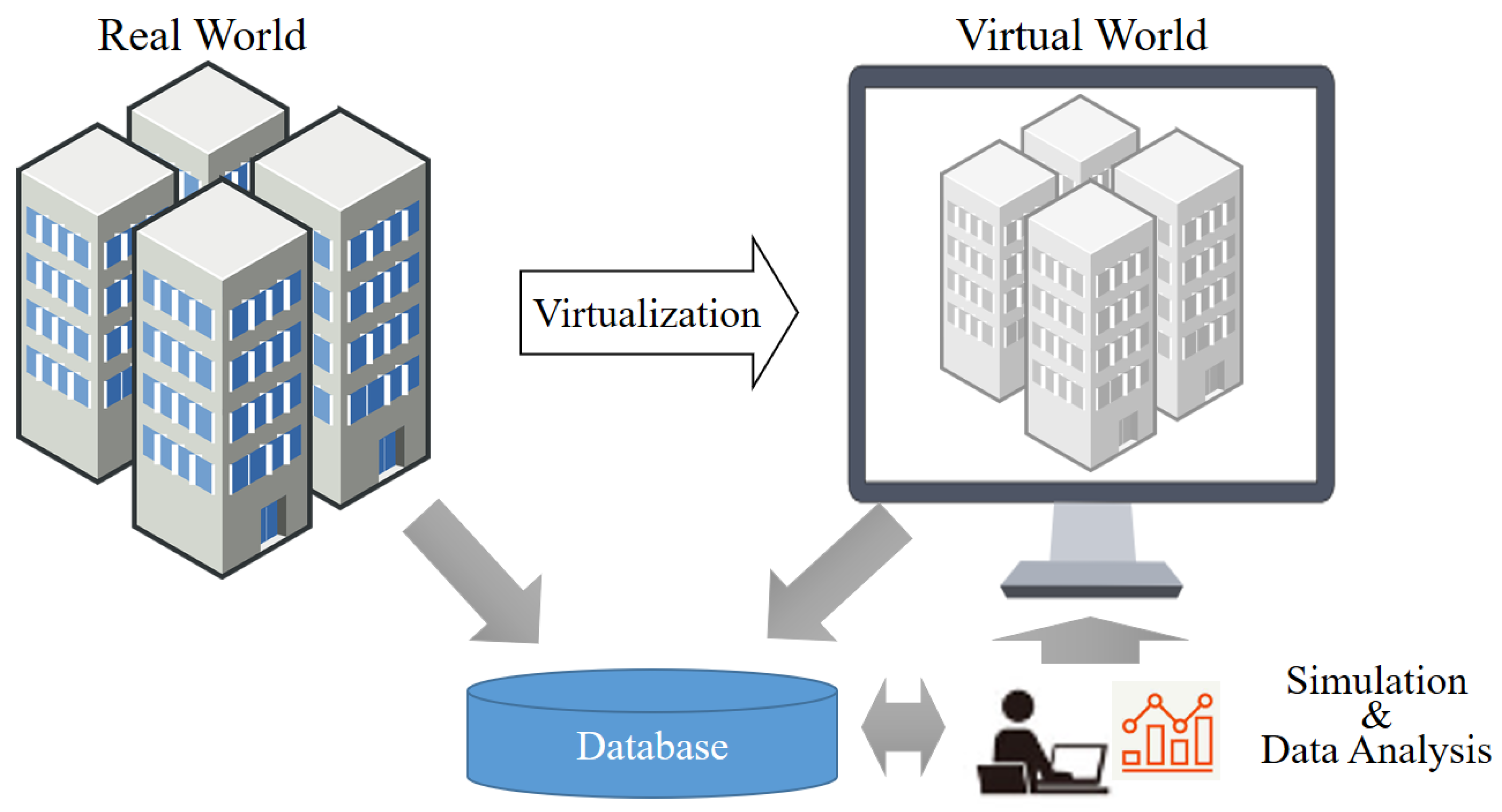
The concept of the digital twin was originally proposed by Michael Grieves of the University of Michigan in 2002, defining it as “a digital product corresponding to a physical product” [8]. Subsequently, NASA (National Aeronautics and Space Administration) further refined the digital twin concept in 2012 [9]. As General Electric of the United States introduced an industrial cloud-based open platform [10], the concept of ‘digitizing a real object, utilizing it, and reflecting the result in reality’ became more refined. Through extensive research and development, it has been elaborated as ‘technology that enables real-time prediction, optimization, monitoring, control, and decision support’ [11]. Figure 1 depicts a technical, conceptual diagram of the digital twin.

Figure 1.
Technical concept of digital twin.
Essentially, before a malware is activated in the physical world, it is analyzed and prevented from causing system malfunctions. Repeatedly implementing a safe physical world within the virtual environment allows for iterative testing and improvement.
In this study, we propose a method to analyze and defend against new types of malware using digital twins.
2.2. Malware
Malware refers to any software that can interfere with or adversely affect the normal operation of an electronic device. As the number of malware rapidly increases, the types of attacks are becoming more diverse and intelligent [12]. According to the 2019 McAfee Labs Threats Report, new malware continues to be discovered, with tens of millions of malware being identified each quarter [13]. Table 1 provides a description of the types of representative malware known so far, along with their characteristics.

Table 1.
Types and characteristics of malware.
2.3. Image Interpolation
Interpolation is a technique used to enlarge or reduce an image. When an image is enlarged, additional pixels must be added between the pixels of the original image. When an image is reduced, one pixel must replace a certain number of pixels in the existing image. Interpolation is distinguished by how pixels are added and how many pixels are mapped to a single pixel.
In this paper, three image interpolation methods were tested: nearest neighbor, bicubic, and bilinear. The detection performance was measured by CNN by adjusting the image size using each interpolation method. In the final proposed system, a method with high performance and short processing time was applied.
The nearest neighbor method is the simplest among interpolation methods and has the shortest processing time. This technique applies the value of the supplemented or replaced pixel to the value of the pixel in the existing image closest to that location. That is, if a two-dimensional image is magnified twice, one pixel is enlarged to 2 × 2 pixels, and the same value as the existing pixel is applied to the value of the 2 × 2 pixel. When an image is reduced by a factor of two, 2 × 2 pixels are replaced with 1 pixel, and the value of one of the existing pixels is applied to the value of the replaced pixel [14]. The bilinear technique considers the four adjacent pixels of a new pixel. The value of the new pixel is determined based on the weighted average of the distances to them. Four pixels are considered, but they are most affected by pixel values of closer distances [15]. The bicubic method considers the 16 adjacent pixels of a new pixel and determines the value of the new pixel based on the weighted average of the distances to them. This technique provides a smoother result and is often preferred for image resizing due to its better preservation of image details and reduced artifacts [16].
2.4. Generative Adversarial Network
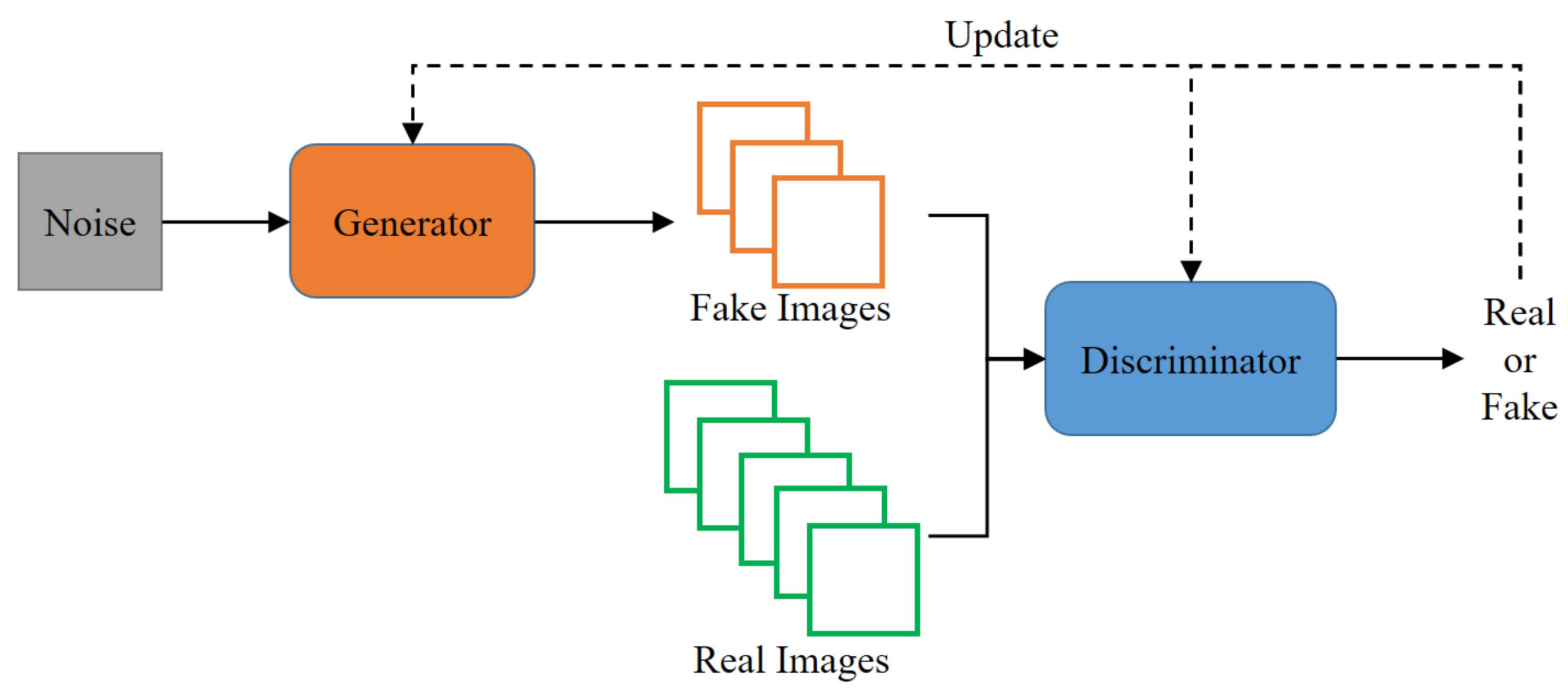
GAN (generative adversarial network) [17,18] consists of a generator/generative model and a discriminator/discriminator model.
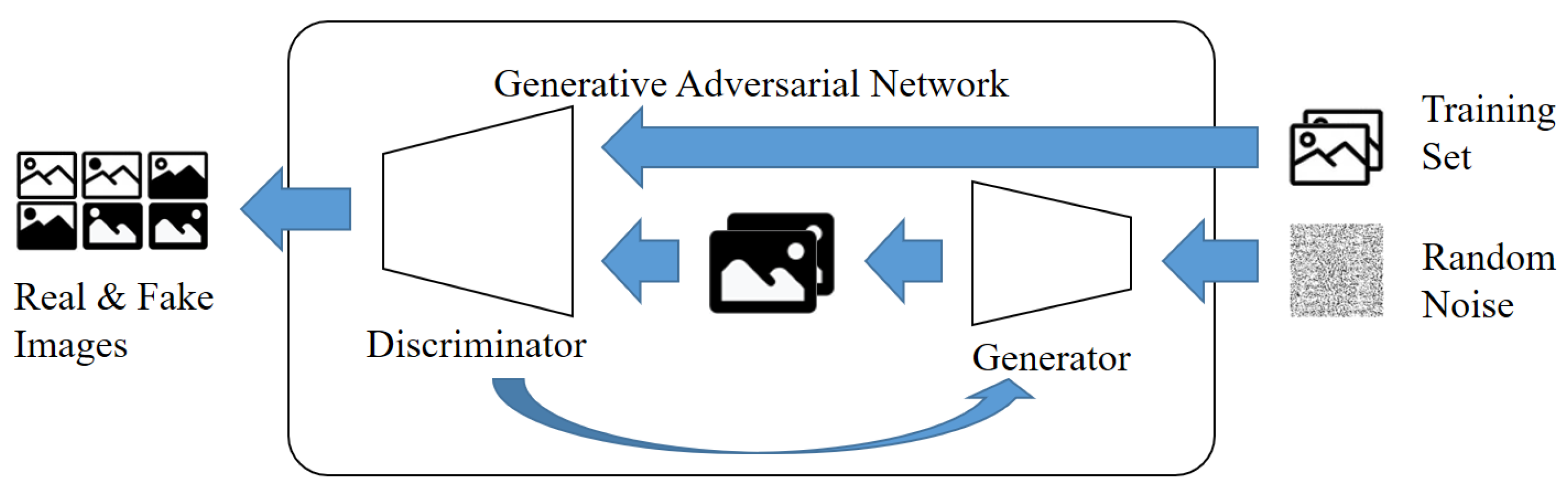
Figure 2 shows the learning structure in a GAN. GANs are often described with examples of banknote counterfeiters and the police. The generator is likened to a banknote counterfeiter, while the discriminator is compared to the police. In this analogy, the criminal (generator) attempts to trick the police (discriminator) with fake banknotes, and the police strive to identify the authenticity of the counterfeit bills. Through this competitive process, each model improves its ability to distinguish between genuine and counterfeit banknotes. As a result, the discriminator (D) tries to make accurate judgments using original data, while the generator (G) generates fake data to prevent the discriminator (D) from making accurate determinations. Through this process of adversarial learning, both models iteratively improve their performance [19].
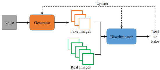
Figure 2.
Learning structure of GAN.
Eventually, the discriminator (D) becomes less able to distinguish between the original data and the fake data generated by the generator (G).
Since GANs are unsupervised, they do not require manual labeling, and by learning the data, they can acquire the internal representation of the data. GANs are capable of generating audio, video, text, and image data that is indistinguishable from real data. As a versatile technology, they find applications in marketing, e-commerce, gaming, advertising, and various other industries.
3. Literature Review
3.1. Digital Twin Application Research
Pokhrel et al. [20] provide a comprehensive overview of research on predicting cybersecurity incidents using digital twin technology. The paper covers the integration of digital twin models and cybersecurity frameworks, machine learning, and data analysis techniques for accident prediction. It also emphasizes the importance of real-time monitoring and anomaly detection in the digital twin context.
Eckhart and Ekelhart [21] conducted a study focusing on the application of digital twins to enhance the security of CPS (cyber-physical systems). The paper reviews the concept of digital twins in the context of CPS security and covers various aspects, such as modeling and simulation capabilities, real-time monitoring, and anomaly detection and analysis.
The proposed technique learns real-time data collected from the physical world of digital twins. Therefore, it provides an environment that can be analyzed safely without affecting systems in the physical world.
3.2. Malware Detection through Imaging
Traditional machine learning techniques such as KNN (k-nearest neighbor) and SVM (support vector machine) were used [22]. However, in recent years, studies that apply deep learning are the main focus. Additionally, the malware detection performance using deep learning is generally superior to that using machine learning techniques [23]. In 2022, Atitallah et al. [24] proposed detection and multiple classification of malware converted into images. The proposed approach combines two machine learning techniques: fine-tuned CNN and random forest voting. This approach takes advantage of CNN’s ability to capture complex patterns in data and random forests, which reduce overfitting and enhance generalization.
However, malware sample images of different classes to which the same packing technique is applied may appear similar. Moreover, limitations arise in terms of generalization error and data imbalance due to the size and diversity of the dataset [25].
In this paper, the malware is expressed in grayscale and converted into an image. Additionally, image interpolation is considered to convert the image into a suitable size for analysis.
3.3. Malware Detection through Machine Learning
In 2009, M. Zubair Shafiq et al. [26] proposed PE-Miner (Portable Executable-Miner), a framework for detecting malware following the PE format (Portable Executable Format) in RAID (Redundant Array of Independent Disks). PE Miner extracts information from PE files and creates vector values. Then, a classification model was proposed through a preprocessing process. For more than 1000 malware, the classification time was reduced to 0.244 s, and a high performance of 99% detection rate was shown.
In 2018, Anderson and Roth [27] proposed Ember, a machine learning model based on machine learning static analysis. Ember extracts information from PE files through static analysis and then creates vector values. A detection model was created using a LightGBM (Light Gradient Boosting Machine) model, which utilizes a boosting technique, a kind of ensemble technique. Ember showed a high detection performance of 92% for more than 800,000 malware.
In 2020, Hojjat Aghakhani et al. [28] published a study on classifying packed malware using static analysis-based features and machine learning-based classifiers. They then created a classification model using a random forest. The study utilized a real dataset consisting of 4396 unpacked normal files, 12,647 packed normal files, and 33,681 packed malicious files. The results showed 41.84% false negatives and 7.27% false positives for the packed dataset. However, it was found to be difficult to accurately classify packed files based solely on static analysis features.
3.4. Malware Detection through Deep Learning
Saxe and Berlin [29] proposed a DNN-based PE file malware detection model. The vector created by analyzing the PE file is used as an input for a deep learning model with two hidden layers. Additionally, the Bayesian model is used to provide the probability of being malicious in addition to detection. The proposed model shows a high detection rate of 95%.
MalConv, proposed in 2017 by Edward Raff et al. [30], is a CNN model that learns without separate feature extraction and preprocessing from PE files. To validate the model, it was verified using two datasets and showed a high accuracy of 93%.
Mahmoud Kalash et al. [31] proposed the M-CNN model at the 2018. M-CNN converts PE files into images and classifies them using convolutional neural networks. The resulting image is classified using the VGG-16 (Visual Geometry Group-16) model. The model was validated using 8394 data points, achieving an accuracy of over 96%.
The proposed system in this paper applies a CNN model through digital twin to safely execute the malware. It converts the binary of a file to a grayscale image. Afterwards, the detection performance is measured for each size and interpolation method to select an appropriate size and interpolation method. Additionally, the detection performance of data generated through adversarial generative neural networks is measured.
4. Materials and Methods
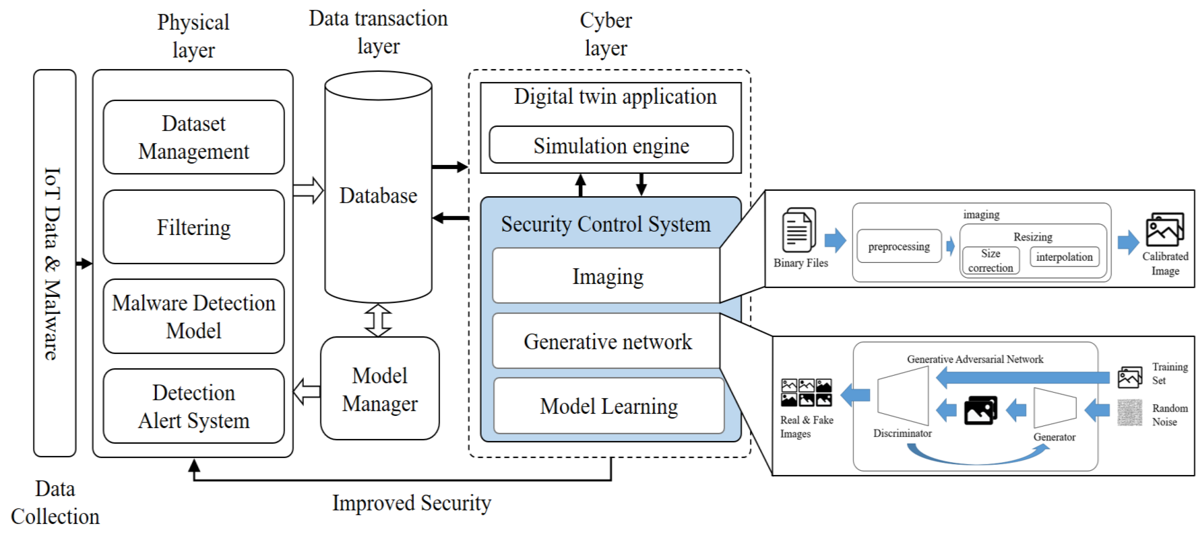
The proposed system is built upon a digital twin-based malware detection system. Figure 3 shows the architecture of the proposed system.
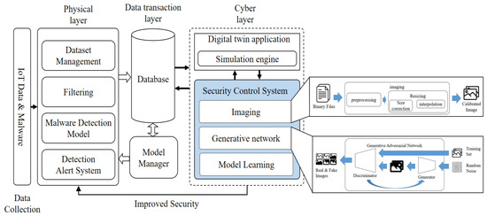
Figure 3.
Digital twin-based conceptual diagram of the proposed system.
The architecture is divided into three layer: physical, data, and cyber. The physical layer represents the anomaly detection system for actual malware, consisting of data collection, analysis, and system management components. The data layer includes a database for storing data and learning models, as well as a system for managing these models. The database stores data collected from the physical layer, malware information, and a learning model that serves as the standard for filtering. The model manager is responsible for managing the learning model based on the stored data. The cyber layer encompasses digital twin applications and security control systems. The digital twin application replicates the actual malware detection system in the virtual world. The security control system is responsible for creating and learning about new types of malware. The learning process is conducted based on information received from the data layer, and the model is updated through interactions with the simulation in the digital twin application, thereby improving the system’s detection capabilities.
The proposed system collects IoT data and classifies it through a malware detection model. While the system can effectively filter known malware in the physical world using pretrained models, it faces limitations in detecting new types of malware that have not been previously learned. To address this challenge, the proposed system leverages the digital world by creating and learning new types of malware based on existing ones. By generating and learning these new malware variants in the digital twin environment, the system enhances its detection capabilities and applies the knowledge gained to the physical world’s detection system. As a result, the proposed system is capable of preemptively detecting emerging threats, surpassing the capabilities of existing methods.
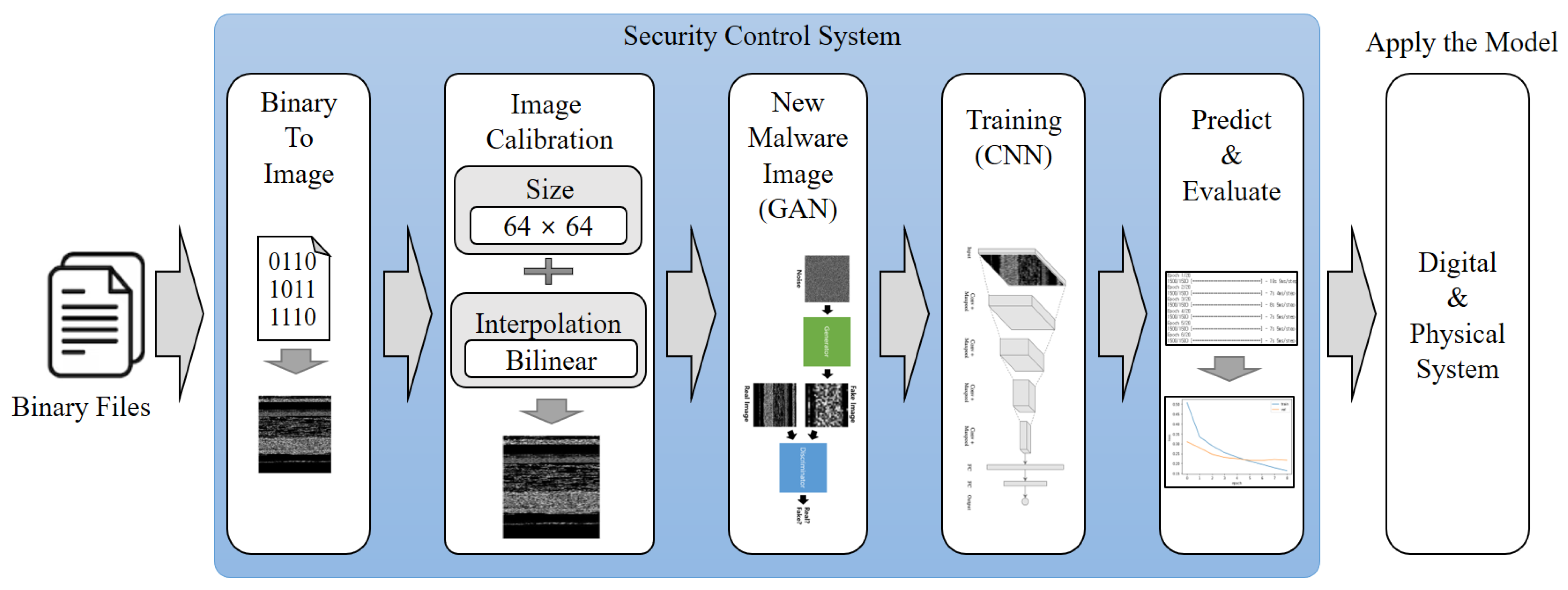
Among the proposed systems, the security control system of the cyber layer is composed of three main components: image generation, new malware image generation, and model learning. Figure 4 illustrates the pre-processing and learning process of the security control system.
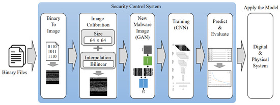
Figure 4.
Pre-processing and learning process of security control system.
The image creation process involves converting an input executable file into an image. To achieve this, the input binary information is digitized and converted into pixel values. Additionally, the image size must be standardized for effective learning. Image correction techniques are employed to prevent information loss during image resizing. In the proposed system, the image size is set to 64 × 64 pixels, and the bilinear method is used for image correction. To determine the optimal image size and correction method, three image sizes (32 × 32, 64 × 64, and 128 × 128) and three correction methods (nearest neighbor, bilinear, and bicubic) are combined. The CNN classification performance is then evaluated to select the most efficient configuration. Next, the new malware image creation process utilizes DCGAN, a generative artificial intelligence technique. This method generates new malware images by extracting characteristics from existing malware images. The generated images are then trained using a convolutional neural network, creating a model capable of detecting malware. This approach enables the system to proactively detect and defend against new types of malware through simulated detection in the virtual environment.
4.1. Imaging of Malware
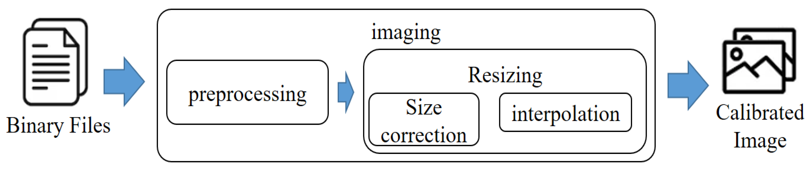
In Figure 5, the process of converting a binary file into an image is depicted. This conversion enables the smooth analysis of malware through image processing. During this process, images of all malware are used as training data after being adjusted to the same size. This step ensures consistency and uniformity in the training data, which is crucial for accurate and effective learning in the subsequent stages of the proposed system.

Figure 5.
Imaging process of malware.
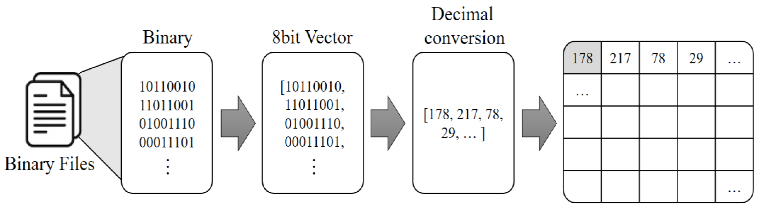
Figure 6 depicts the pre-processing process of converting a malware into an image. In this process, the size of the image is not a primary concern. The binary data of the malware file is read as a vector of 8-bit unsigned integers. Subsequently, each byte is converted into one pixel of the image, with values ranging from 0 to 255, creating a grayscale image. The size of the image is determined based on the file size. Therefore, the width and height of the image are calculated as the square root of the total number of bytes [32]. As the file size varies, the size of the converted image will also differ accordingly.
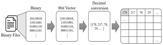
Figure 6.
Imaging pre-process of malware.
For training purposes, all images used as inputs to the deep learning model must be of the same size. Therefore, the malware image is resized to a specific size after the pre-processing phase. During this process, it is crucial to adjust the size while preserving the essential characteristics of the image as much as possible. Interpolation is employed to resize the image while maintaining its overall shape. Depending on the interpolation method applied and the desired size for conversion, the shape of the image may slightly vary. In the proposed system, an experiment was conducted to assess the detection performance based on different image sizes and interpolation methods. The image size options included 32 × 32, 64 × 64, and 128 × 128, while interpolation methods considered were nearest neighbor, bilinear, and bicubic. Larger image sizes generally lead to better detection performance, but it comes at the cost of increased processing time. Hence, in the proposed system, the image size was standardized to 64 × 64 using bilinear interpolation, striking a balance between performance and efficiency.
4.2. Data Augmentation through Generative Adversarial Networks
The generative model of the proposed system uses DCGAN. The process of creating a new malware image is shown in Figure 7. In the generative model of the proposed system, there is one generator and one discriminator. The generator considers as input an image made of random noise, while the discriminator receives the malware image and the image created by the generator to determine their authenticity. Malware images are generated by converting binary files into images, and then resizing them to 64 × 64 size. Among these images, we divide them into a training set and a test set to evaluate the system’s performance.
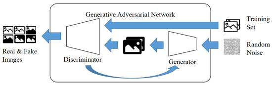
Figure 7.
Process of creating malware images.
The discriminator’s goal is to predict whether an image is real or fake. This is similar to an image classification problem in supervised learning. Therefore, it is possible to use a network structure in which convolutional layers are stacked, and the output layer serves as the connection layer. The structure of the discriminator model in the proposed system is illustrated in Figure 8.
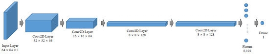
Figure 8.
Composition of the discriminator model of the proposed system.
The input is an image of size 64 × 64. The first convolutional layer, Conv2D, employs 64 filters, reducing the feature map size to 32 × 32. In the second convolutional layer, 64 filters are used, further reducing the feature map to 16 × 16. Subsequently, the third convolutional layer utilizes 128 filters, resulting in an 8 × 8 feature map. The last convolutional layer also employs 128 filters, preserving the 8 × 8 feature map size. The feature map is then flattened and converted into a vector. Passing through a dense layer with a single unit, the output is transformed into a value between 0 and 1. This model considers an image as input and outputs a number that distinguishes real from fake. Next, we consider the number of parameters in the discriminator. The first convolutional layer contains 64 filters, resulting in 1664 parameters. The second convolutional layer, with 64 filters, contributes 102,464 parameters. The third convolutional layer employs 128 filters and adds 204,928 parameters. Finally, the last convolutional layer has 128 filters and 409,728 parameters. When these parameters are flattened and connected as a single unit, the count becomes 8193. The total number of discriminator parameters sums up to 726,977.
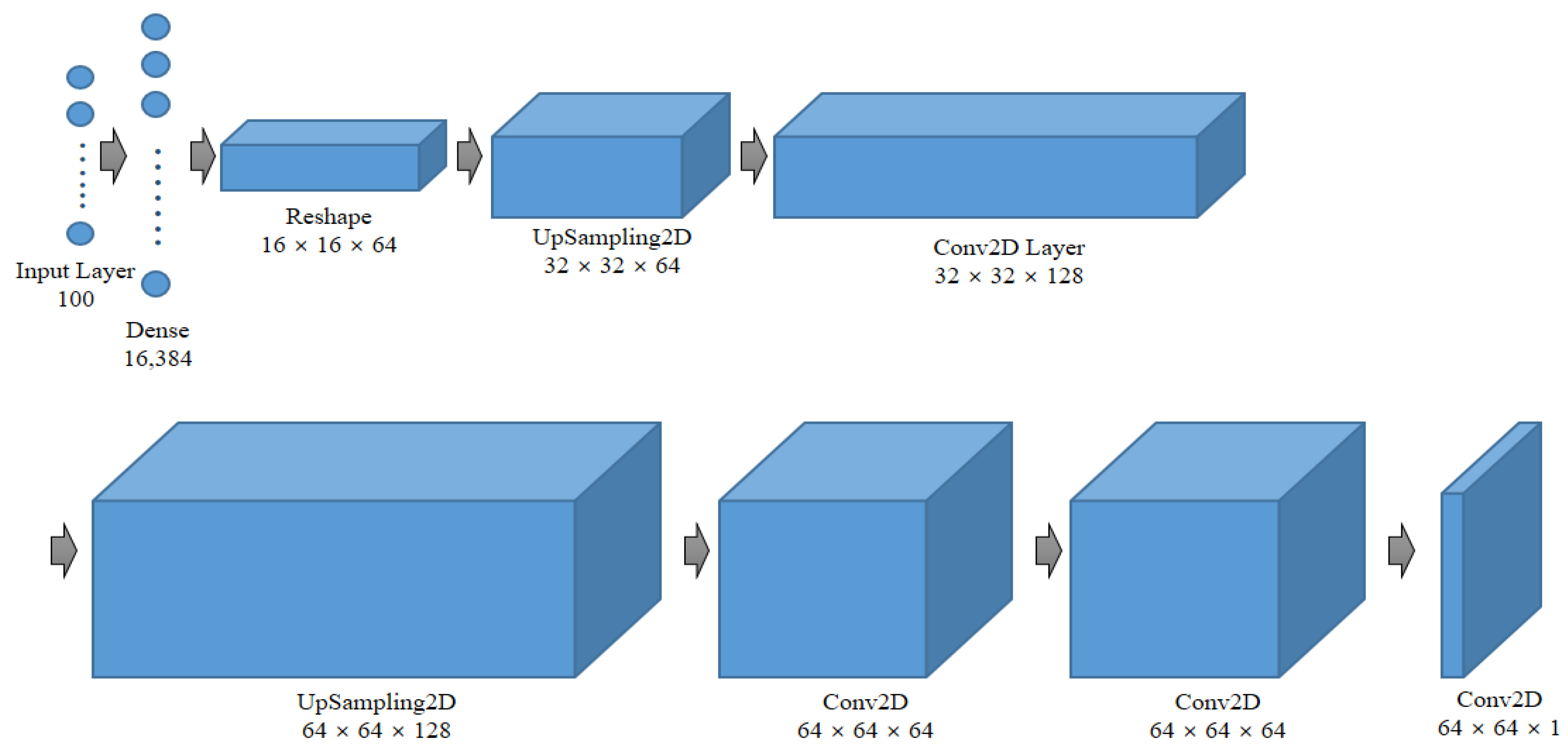
The generator typically considers a vector sampled from a multivariate standard normal distribution as input and produces an image of the same dimensions as the original training data. Its role is to transform latent space vectors into images. The structure of the proposed system’s generator model is illustrated in Figure 9.

Figure 9.
Configuration of the generator model of the proposed system.
The constructor considers a vector of length 100 as input and passes it through a dense layer with 16,384 units. Batch normalization and ReLU activation functions are applied to transform the feature map into a size of 16 × 16 with 64 filters. Subsequently, an upsampling layer increases the feature map to 32 × 32. The first convolutional layer uses 128 filters. Another upsampling layer increases the feature map to 64 × 64. Through two additional convolutional layers with 64 filters, a final 64 × 64 feature map is obtained, which matches the size of the original image. This model considers a vector of length 100 as input and outputs a 64 × 64 image. Next, let us consider the parameter sizes of the constructor model. The initial input of 100 vectors is connected to 16,384 neurons, resulting in 1,654,784 parameters. After applying batch normalization, there are 65,536 parameters. The first convolutional layer has 204,928 parameters, and after applying batch normalization, there are 512 parameters. The second convolutional layer contains 204,864 parameters, and batch normalization contributes 256 parameters. The third convolutional layer has 102,464 parameters. Lastly, the final convolutional layer adds 1601 parameters. The total number of parameters is 2,235,201. Among them, 33,280 parameters are unlearned, leaving 2,201,921 parameters used for learning.
4.3. Deep Learning Model for Malware Detection
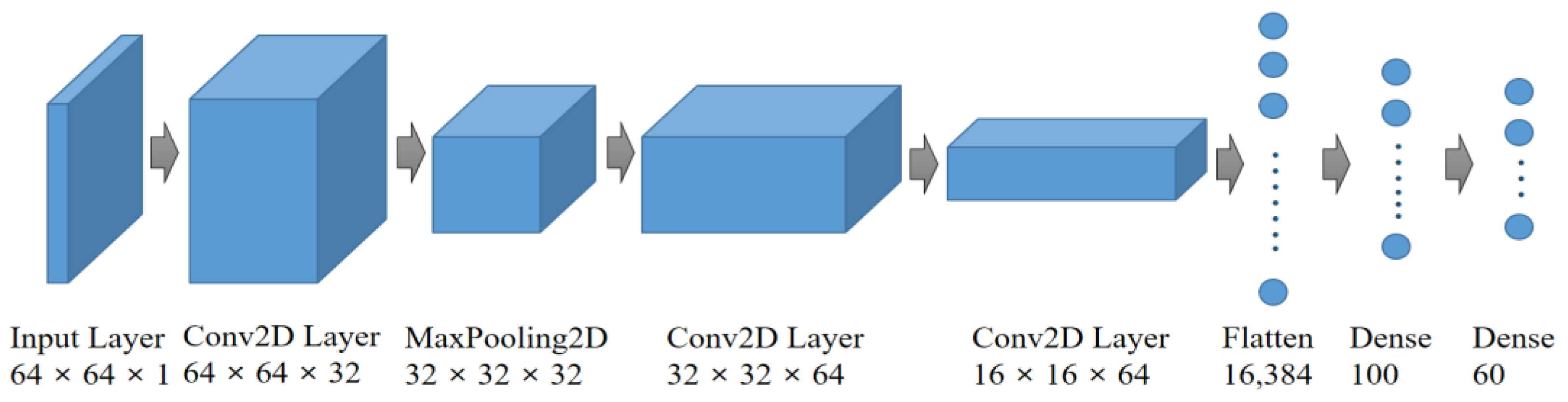
The proposed system’s malware detection model utilizes a convolutional neural network (CNN) architecture. The model’s structure is illustrated in Figure 10. It consists of a series of layers, including a convolutional layer, a pooling layer, and a Rectified Linear Unit (ReLU) activation function.
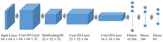
Figure 10.
Composition of malicious code detection model.
In the convolutional layer, the model performs convolutions on the input data to extract relevant features. The pooling layer reduces the spatial dimensions of the feature maps, aiding in feature extraction and dimensionality reduction. Additionally, the ReLU activation function introduces non-linearity to the model, enhancing its capacity to capture complex patterns and relationships in the data.
The model receives an input of size 64 × 64. The first convolutional layer, Conv2D, employs 32 filters with the ReLU activation function. Subsequently, a pooling layer is added, reducing the feature map size to 32 × 32. Moving on, the second convolutional layer and pooling layer use 64 filters, resulting in a feature map size of 16 × 16. The 3D feature maps are then flattened to facilitate feature classification. To prevent overfitting, a dense hidden layer and an output layer are added, enabling multi-classification into 60 categories. For the experiments using the Mal60 dataset, the model classifies 60 types of malware. In the case of Malimg, the classification is adjusted to 25 types. To calculate the number of parameters in the model, the first convolutional layer with 32 filters has 320 parameters. The second convolutional layer with 64 filters contributes 18,496 parameters. Flattening the feature maps and connecting them with 100 neurons results in 1,638,500 parameters. The total number of parameters in the model sums up to 1,663,376.
5. Experiment
5.1. Experimental Data
The proposed model was validated using three datasets. The first dataset is the Malimg dataset [33], which was also utilized in previous studies by Kamundala and Kim [34], AlGarni et al. [35], Go et al. [36], and Bhodia et al. [37]. The second dataset used is the Mal60 dataset [38], as studied by Kang and Kim [39]. The last dataset was VXHeaven’s 2010 virus collection dataset [40].
The Malimg dataset used in malware imaging research is categorized into 25 families. The dataset comprises a total of 9458 malware samples. However, for the purpose of this paper, which focuses on classification with a limited number of samples, only 20 samples were randomly selected from each family, resulting in a total of 500 samples in the composed dataset.
The Mal60 dataset used in this research is classified into 60 families, each containing a total of 20 malware samples, resulting in a dataset size of 1200 samples. Notably, each family represents a unique category of malware. In some cases, different security companies may assign different names to the same family of malware based on their naming criteria. However, despite these naming differences, the code samples are classified under the same group as they exhibit similar malicious behavior or characteristics. Additionally, certain malware samples in Kaspersky and Bitdefender products may have diagnosis names that cannot be confirmed or are classified as heuristic diagnosis names. Specifically, two examples of such samples are identified as belonging to the Akdoor and Rifdoor families, targeting specific areas.
The VXHeaven dataset comprises 270 k malware executable files, but it does not include malware family information. To determine the family of each sample in the VXHeaven dataset, we added family labels through Virustotal [41], a malware analysis site. When a suspected malware file is uploaded to Virustotal, the site analyzes it for family prediction using various antivirus engines. The malware family label is assigned based on the results obtained from the Microsoft Antivirus engine.
A total of 70% of each dataset is used for training, and the remaining 30% for testing.
5.2. Experiment Environment
The proposed system underwent testing by dividing it into two stages: the imaging stage and the data generation stage. In the imaging stage, the detection performance was measured for each image size and correction method. Additionally, in the data generation stage, data was generated, and the detection performance of the generated data was measured.
To ensure a robust and efficient experimental environment, the experiments were conducted using Google Colaboratory’s GPU environment, which helped overcome the limitations of local environments and enabled consistent research in the same environment. The hardware environment and experimental setup used for learning and implementing the model are summarized in Table 2.
Table 2.
Experiment environment.
5.3. Experimental Setup of Imaging
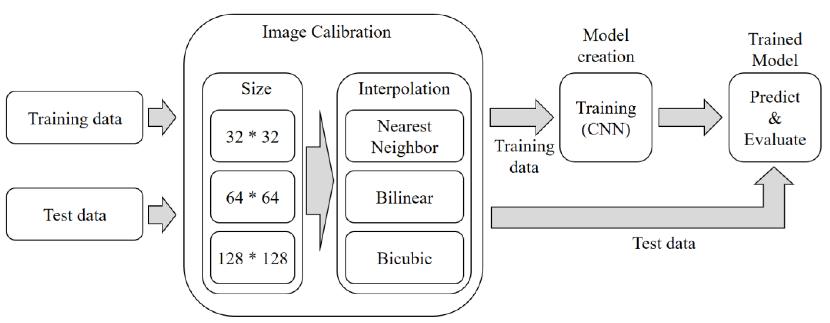
The experimental procedure, as depicted in Figure 11, involves the following steps: Step 1. Data Preparation: The training data and test data are adjusted to create nine different cases based on the image size (32 × 32, 64 × 64, 128 × 128) and interpolation method (nearest neighbor, bilinear, and bicubic).
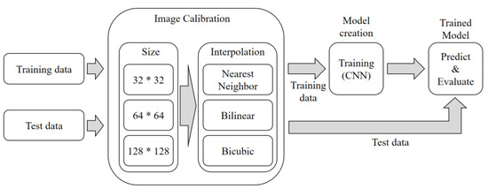
Figure 11.
Experimental process of imaging.
Step 2. Model Training: The adjusted training data is used to train a CNN-based deep learning model. As a result, nine different models are generated, each corresponding to a specific combination of image size and interpolation method. During the training process, a batch size of 128 is used, and the learning is repeated for 200 epochs.
Step 3. Model Evaluation: Evaluation of the models is performed separately for each image size. First, a sample image is tested to verify the model’s performance. Then, the test is conducted using malware samples. By following this experimental procedure, we can assess the detection performance of the CNN-based models under various settings, such as different image sizes and interpolation methods.
5.4. Experimental Setup of Data Augmentation through Generative Adversarial Networks
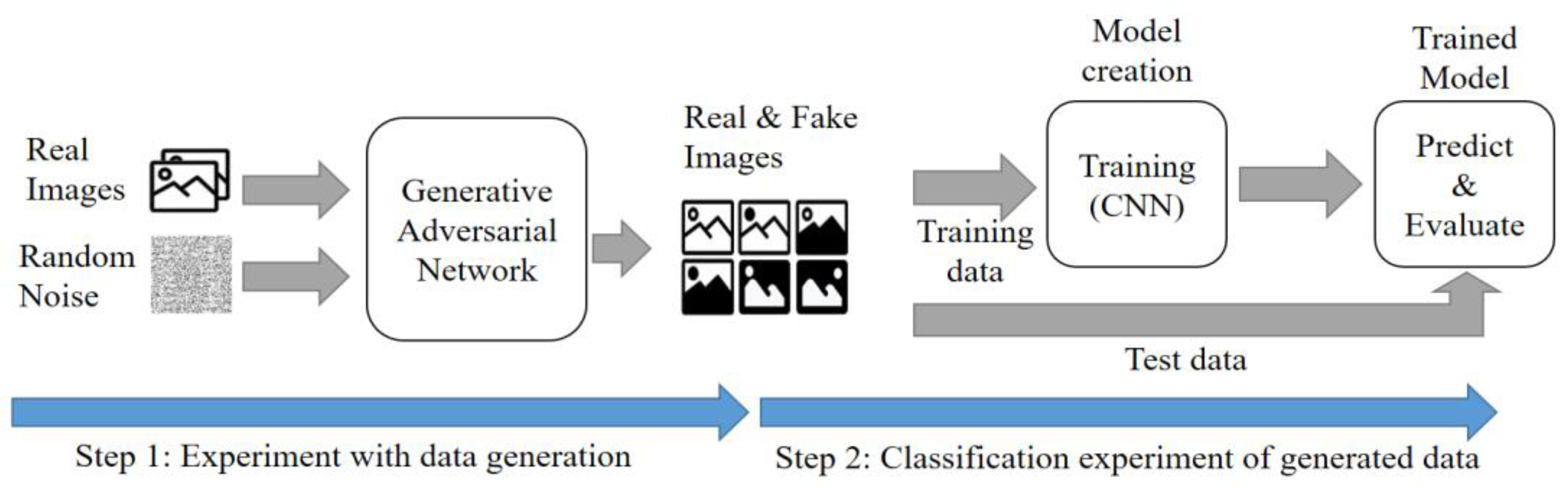
The experimental procedure is shown in Figure 12. The image required for the experiment determines the size and correction method based on the results of the imaging experiment. Therefore, the experiment is conducted using a 64 × 64 size image with good performance results, corrected by the bilinear method. The experiment proceeds in two stages. The first step involves the similarity evaluation for fake images generated using GAN. Step 2 is the CNN performance evaluation for both existing data and generated data.

Figure 12.
Data generation experiment process.
Step 1 involves creating a new image using DCGAN. The image created in the preprocessing process has a size of 64 × 64 pixels, and the image generated by DCGAN is also 64 × 64 pixels. The time taken to create the image increases with higher resolution. The evaluation assesses the similarity between the real and generated images, using factors such as FID (Fréchet Inception Distance) and the cross-correlation coefficient. Additionally, the loss value is checked to ensure that mode collapses are minimized during creation. The batch size was set to 128, and the learning process was repeated 20,000 times.
In the second step, the detection performance of the generated images and the existing images, which are the results of the first step, is measured. The detection process uses the same CNN model as used in the imaging experiment. The experiment evaluates the detection performance of the generated images. The training and test images are classified in a ratio of 8:2. Evaluation factors include precision, recall, f1-score, and accuracy. The batch size is set to 128, and the learning process is repeated 200 times.
6. Performance Evaluation
6.1. Performance Evaluation of Imaging
When a malicious code file is expressed as an image, the width or length of the image is usually fixed to a certain size. Since the file size of the malicious code is different, the size of the converted image also appears in various ways. Figure 13 shows only a portion of the results of converting malicious code into an image. Malicious code images are converted into images with a fixed length. In other words, it can be seen that Adialer.C malware is the largest. And Agent.FYI malware has the smallest size.

Figure 13.
Sample images from the Malimg dataset. (a) Adialer.C, (b) Agent.FYI, (c) Allaple.A, and (d) Allaple.L.
For training purposes, all images utilized as inputs for the deep learning model need to share the same dimensions. Consequently, the malicious code images are transformed to a predetermined size. During this process, interpolation is employed to adjust the size while preserving the image’s characteristics to the greatest extent possible. Nearest neighbor, bilinear, and bicubic techniques are employed for image refinement. Nearest neighbor, although simple and swift, sacrifices visual quality, resulting in jagged edges, particularly during magnification. This technique is straightforward to implement and comprehend, suitable when prioritizing speed and accepting some degree of quality loss. The bilinear technique yields smoother outcomes but may lack sharpness, potentially leading to slightly blurred edges. It is slower than nearest neighbor but remains a fast method, delivering superior quality compared to the former and serving well for general-purpose scaling. On the other hand, the bicubic technique affords the highest quality but comes with increased computational complexity. This involves intricate calculations, typically considering 16 adjacent pixels. Bicubic produces considerably smoother images than bilinear and is the preferred choice for high-quality resizing, especially when maintaining sharpness is crucial.
Table 3 showcases the results of time measurements required for image conversion. The time needed was gauged with respect to each interpolation method. A total of 2210 malware images were utilized for time assessment, with time measured in seconds. The results of the measurements were presented with two decimal places. The outcomes illustrate that computation time diminishes in the sequence of nearest neighbor, bilinear, and bicubic techniques.
Table 3.
Time required for each interpolation method.
Table 4 present the f1-score results for imaging. Overall, the detection performance is relatively better when bilinear or bicubic interpolation methods are applied than when nearest neighbor is used. Additionally, the larger the size of the image, the better the detection performance. However, selecting the optimal interpolation method and image size to be applied to the model should not be solely based on detection performance. It is essential to consider other factors, such as computation requirements. As the size of the image increases, the amount of computation also increases, with bilinear and bicubic methods requiring more computation than nearest neighbor. Therefore, depending on the type of service to be implemented, the interpolation method and image size must be selected, taking into consideration both detection performance and processing time. In this paper, a data generation experiment was conducted using 64 × 64 size images and the bilinear interpolation method. The average accuracy of the entire experiment was 98.2%, the average precision was 96.5%, and the average recall was 97.5%.
Table 4.
F1-score analysis results.
Figure 14, Figure 15 and Figure 16 are some of the results of creating an image and adjusting its size using a correction method.
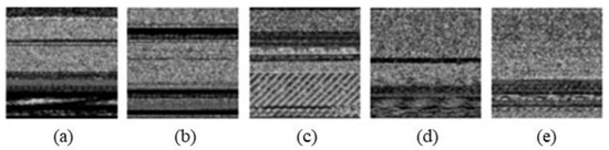
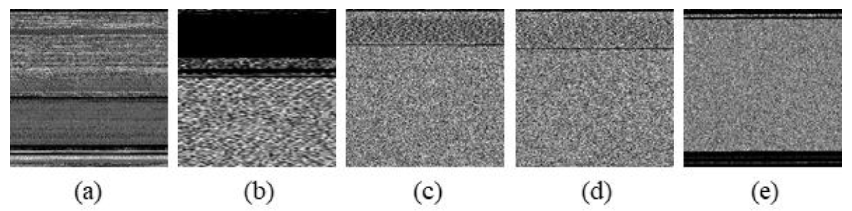
Figure 14.
Sample image from Mal60 dataset. (a) Abnores, (b) Adposhel, (c) Akdoor, (d) CRyptXXX, and (e) Downloader.

Figure 15.
Sample image from Malimg dataset. (a) Adialer.C, (b) Agent.FYI, (c) Allaple.A, (d) Allaple.L, and (e) Alueron.gen!J.

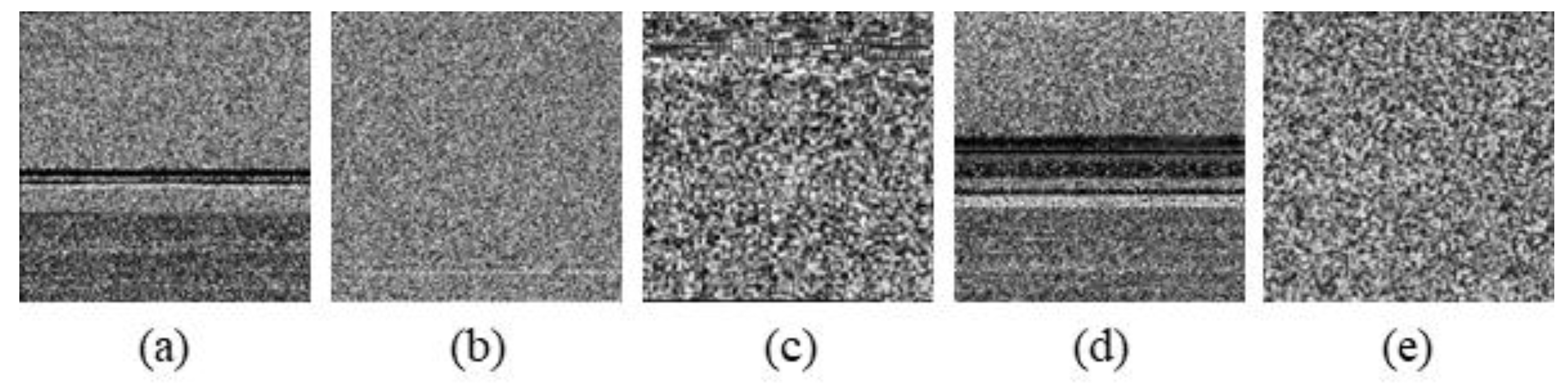
Figure 16.
Sample image from VXHeavens dataset. (a) C2Lop.A, (b) Helpud.A, (c) Treemz.gen!A, (d) Seimon.D, and (e) Storark.A.
6.2. Performance Evaluation for Data Generation
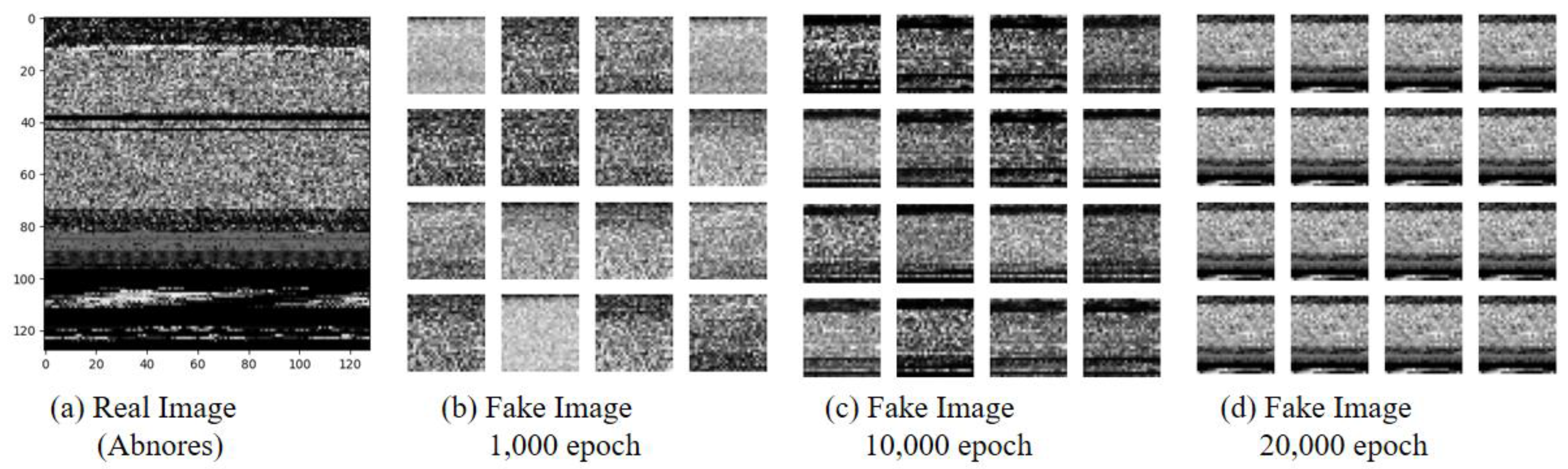
For data generation, training was performed with 20,000 epochs, and this study was repeated four times. Figure 17 shows the progression of fake images generated from the generative network during the learning process. Figure 17a represents the real image of the Abnores type among malware. Subsequent images, Figure 17b–d, depict the results at 1000, 10,000, and 20,000 epochs, respectively.
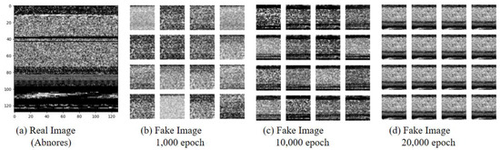
Figure 17.
Fake image according to epochs.
At 1000 epochs, the generated fake images lack proper features and exhibit a noticeable presence of different noise patterns compared to the real images. As training progresses to 10,000 epochs, the ambient noise in the generated images starts to somewhat resemble the real images. Finally, at 20,000 epochs, we can observe a significant improvement, with the generated images exhibiting a closer resemblance to the real images. This iterative learning process demonstrates that with sufficient training, the generative model can achieve images that are more similar to the real ones.
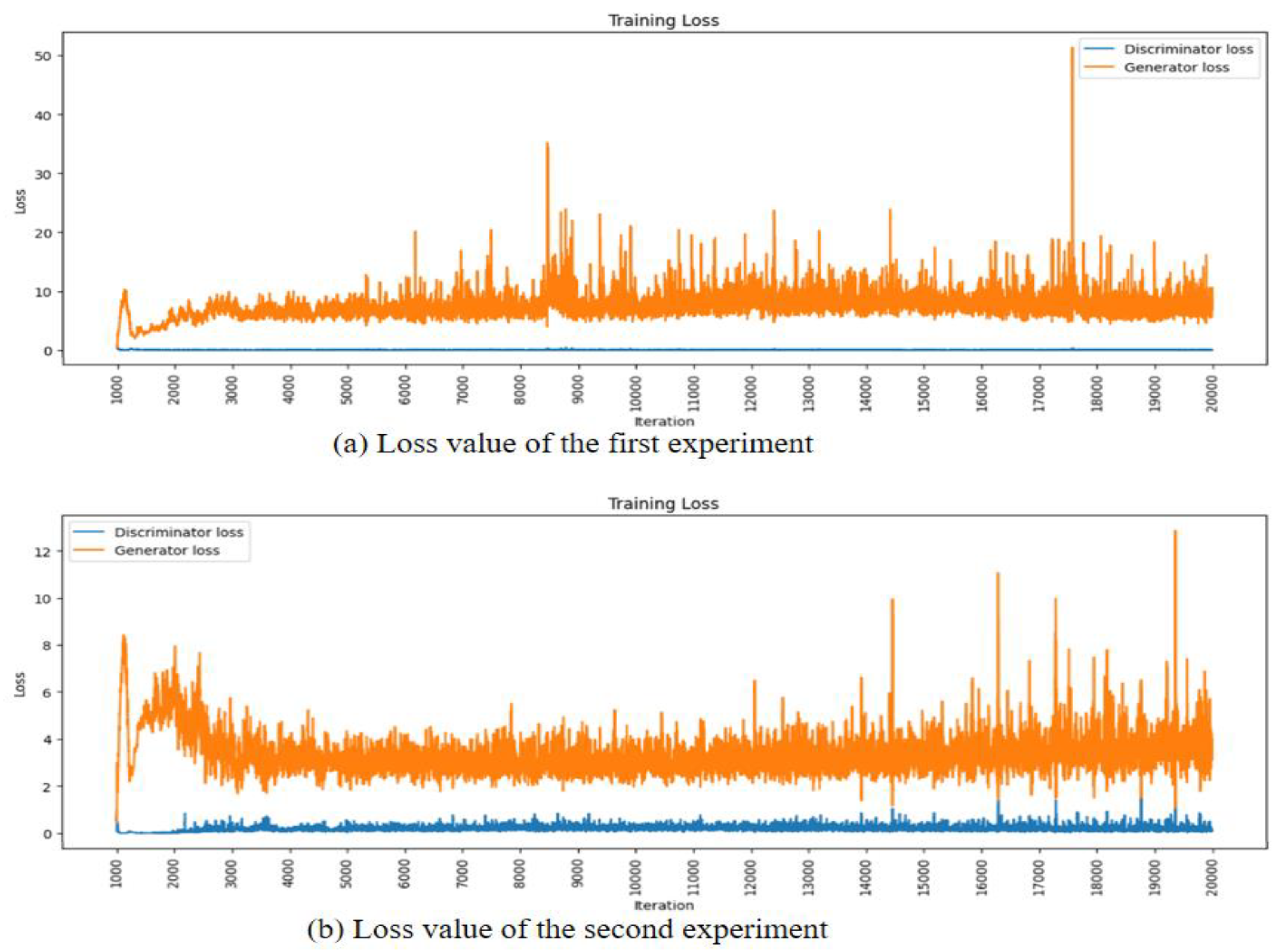
Figure 18 depicts the loss values of the generator and discriminator during the data generation process. In both the first and second experiments, we observe that the generator loss value stabilizes around 3000 epochs. This indicates that the model is progressing without experiencing mode collapse during the generation of data. Mode collapse occurs when the generator fails to produce diverse samples and is stuck generating only a limited set of outputs. The stable loss values suggest that the training process is robust, ensuring that the generator continues to generate diverse and meaningful data throughout the epochs.

Figure 18.
Loss value of generative model.
Table 5 presents the FID and cross-correlation values for each count. A smaller FID value indicates that the model generates data more similar to the original data. The average FID index obtained is 5.4603, which suggests that the generated data is relatively similar to the original data. Additionally, the average correlation coefficient is 0.8898, indicating a high degree of similarity between the original data and the generated data. These results, along with the FID, demonstrate that the generative model has successfully produced data that closely resembles the characteristics of the original data.
Table 5.
FID and cross-correlation for each count.
6.3. Detection Performance Evaluation of Generated Data
CNN was used to verify the usability of the data generated using the generative model. Training was conducted by constructing generated images and noise images. The test for verification consisted of images not used in the generative model, generated images, and noise images. The CNN model for learning the generated image used the same model as Figure 11. This is the same model that tested the detection performance of the image size.
The model’s performance is presented in Table 6, using evaluation indices such as accuracy, precision, recall, and f1-score. The training results demonstrate high performance, achieving an accuracy of approximately 0.98, a precision of 0.94, a recall of 0.96, and an f1-score value of 0.95 when training was conducted solely with generated images. However, the detection performance using the test set appears to be relatively lower. This can be attributed to the fact that the model was well-trained to distinguish the characteristics of the images during the training stage. Moreover, the inclusion of both malware and normal images in the practice may lead to slightly lower performance for detecting normal images. Nevertheless, the overall training results indicate promising performance, showcasing the model’s ability to accurately classify and distinguish between different image types.
Table 6.
Performance comparison results.
Table 7 presents the results of the comparison with other models. It has been observed that the accuracy of our model surpasses that of previous studies. While precision, recall, and f1-score were only available in certain studies, our model still exhibited superior performance compared to the previous approaches.
Table 7.
Performance comparison with existing research.
The proposed model offers several distinct advantages over simulation in a digital twin environment. First, it demonstrates the ability to effectively detect new malware that did not exist before and combat new threats. Second, the detection model is trained without separate pre-work for the detection model. Unlike previous studies, our model simplifies the overall workflow by eliminating the need for feature extraction via specific filters or APIs. Third, it simplifies and streamlines the process by eliminating the requirement to directly run the model in a separate sandbox.
Leveraging these advantages, our proposed model represents a significant advance in malware detection, providing a more streamlined and robust approach compared to existing methods in the field. Simulation results of the digital twin environment demonstrate the robustness and effectiveness of the proposed model in protecting against evolving threats.
7. Discussion
In this paper, we present an innovative intelligent detection technology that leverages generative neural networks within a digital twin-based Industrial Internet of Things (IIoT) environment. Moreover, we propose a novel method for detecting malware solely based on images of the malware using convolutional neural networks (CNN), which is a powerful technique employing deep neural networks.
Three different datasets were used to test the performance of the proposed system. The performance of the system was measured in three stages. First, in the imaging stage, the detection performance of the 64 × 64 bilinear technique was the best. Second, a new malware image was created using the image interpolation method and size determined in the previous experiment, and similarity with the original images was measured. As a result of the measurement, the FID index was 5.4403 and the correlation coefficient was 0.8698, confirming high similarity. Third, the malware detection performance using the generated malware image was measured. The performance measurement result was detected with an accuracy of 0.97, and was measured with a precision of 0.93, a recall of 0.94, and an f1-score of 0.94. This confirmed a higher level of performance than previous studies.
The proposed system does not analyze the data collected in the IIoT environment on the user’s system. Instead, it utilizes the digital twin to analyze malware in the digital space. As a result, it does not adversely affect the actual system, providing a safer and more secure analysis environment. Additionally, the system offers the advantage of quick initialization if any problem occurs in the digital space. By converting malware into images that reflect their characteristics, the proposed system eliminates the need to execute or directly analyze the code, minimizing potential risks. Leveraging generative adversarial networks allows for the generation of synthetic malware, which enhances the efficiency of the analysis process. The unpredictable nature of when and in what form malware will emerge poses a challenge for traditional detection methods. However, in the digital twin environment, the proposed system can quickly respond to new forms of malware by generating and analyzing them based on existing malware. This adaptability and responsiveness make the system well-suited for addressing emerging threats in the digital space.
The table provided below (Table 8) illustrates the datasets that will be contrasted with the research findings presented in Table 7. In this paper, the Mal60 dataset, the Malimg dataset and the VXHeaven dataset were employed. To enable an objective comparison of studies, we utilized datasets from prior research. The datasets from earlier studies predominantly comprise data made available from 2010 to 2015.
Table 8.
Dataset status of research for performance comparison.
This study has certain limitations. During the image downsizing process aimed at reducing computational complexity, some intricate characteristics of the malicious code may diminish. Detection can be influenced by various factors such as the chosen image interpolation method, image size, and the aspect ratio of image width and height. Additionally, accuracy can be compromised when the flows and patterns of malicious codes exhibit similarity only in minute sections. Moreover, augmenting the model’s reliability necessitates training it with a contemporary and comprehensive dataset.
8. Conclusions
Research efforts persist in the realm of malicious code detection. Prior investigations have involved feature extraction through methods like image conversion or direct analysis of PE files for malicious code detection. Conversely, the exploration of techniques for real-time detection within virtual machines has also been pursued. Notably, there has been a surge in research centered on detection through machine learning technologies. Nonetheless, the extraction of feature points constitutes an additional requisite step. Furthermore, the analysis conducted within a user’s system might potentially trigger system-related issues, thus presenting a drawback. Machine learning, by its nature, necessitates substantial volumes of data.
Therefore, in this study, an intelligent detection technology was introduced within a digital twin environment that replicates the real-world scenario digitally. By operating within a separate space from the actual system, this approach ensures no impact on the genuine system. Moreover, even in the event of an issue, swift reinitialization is feasible. Among the techniques harnessing deep neural networks for detection, convolutional neural networks (CNN) are utilized to identify malicious code solely using images of such code. Additionally, generative neural networks were employed to augment insufficient malicious code data or generate new instances of malicious code data. A comparison was conducted against seven models from previous studies. The results indicated that the proposed system achieved an f1-score of 0.94, showcasing the effectiveness of the proposed approach. The system exhibited a slightly favorable performance outcome.
In the future, our research will focus on developing technologies capable of surmounting and rectifying the aforementioned limitations. In pursuit of this objective, we will analyze the correspondence between the technique of categorizing malicious code by its function and representing it through intricate images, and the disassembly code associated with each function. Furthermore, we will explore methods to avert the loss of intricate features during image correction. Additionally, we plan to undertake supplementary investigations that encompass other factors, including the horizontal and vertical ratios of images.
Author Contributions
Conceptualization and methodology, H.-J.C., H.-K.Y., Y.-J.S. and A.R.K.; validation, Y.-J.S. and A.R.K.; formal analysis, H.-J.C. and H.-K.Y.; resources, H.-K.Y.; supervision, Y.-J.S. and A.R.K.; writing—original draft preparation, H.-J.C.; writing—review and editing, H.-K.Y., Y.-J.S. and A.R.K. All authors have read and agreed to the published version of the manuscript.
Funding
This research was supported by the MSIT (Ministry of Science and ICT), Korea, under the Innovative Human Resource Development for Local Intellectualization support program (IITP-2023-RS-2022-00156334) supervised by the IITP (Institute for Information & communications Technology Planning & Evaluation).
Institutional Review Board Statement
Not applicable.
Informed Consent Statement
Not applicable.
Data Availability Statement
Not applicable.
Conflicts of Interest
The authors declare no conflict of interest.
References
- Peter, O.; Pradhan, A.; Mbohwa, C. Industrial internet of things (IIoT): Opportunities, challenges, and requirements in manufacturing businesses in emerging economies. Procedia Comput. Sci. 2023, 217, 856–865. [Google Scholar] [CrossRef]
- Sobb, T.; Turnbull, B.; Moustafa, N.; Sobb, T.; Turnbull, B.; Moustafa, N. Supply chain 4.0: A survey of cyber security challenges, solutions and future directions. Electronics 2020, 9, 1864. [Google Scholar] [CrossRef]
- Vaza, R.N.; Prajapati, R.; Rathod, D.; Vaghela, D. Developing a novel methodology for virtual machine introspection to classify unknown malware functions. Peer-to-Peer Netw. Appl. 2022, 15, 793–810. [Google Scholar] [CrossRef]
- Vasan, D.; Alazab, M.; Wassan, S.; Safaei, B.; Zheng, Q. Image-Based malware classification using ensemble of CNN architectures (IMCEC). Comput. Secur. 2020, 92, 101748. [Google Scholar] [CrossRef]
- Shaukat, K.; Luo, S.; Varadharajan, V. A novel deep learning-based approach for malware detection. Eng. Appl. Artif. Intell. 2023, 122, 106030. [Google Scholar] [CrossRef]
- Shorten, C.; Khoshgoftaar, T.M. A survey on image data augmentation for deep learning. J. Big Data 2019, 6, 60. [Google Scholar] [CrossRef]
- Berg, S.; Kutra, D.; Kroeger, T.; Straehle, C.N.; Kausler, B.X.; Haubold, C.; Schiegg, M.; Ales, J.; Beier, T.; Rudy, M. Ilastik: Interactive machine learning for (bio) image analysis. Nat. Methods 2019, 16, 1226–1232. [Google Scholar] [CrossRef]
- Grieves, M. Digital Twin Certified: Employing Virtual Testing of Digital Twins in Manufacturing to Ensure Quality Products. Machines 2023, 11, 808. [Google Scholar] [CrossRef]
- Wu, J.; Yang, Y.; Cheng, X.; Zuo, H.; Cheng, Z. The development of digital twin technology review. In Proceedings of the 2020 Chinese Automation Congress (CAC), Shanghai, China, 6–8 November 2020; pp. 4901–4906. [Google Scholar] [CrossRef]
- Lo, C.; Chen, C.; Zhong, R.Y. A review of digital twin in product design and development. Adv. Eng. Inform. 2021, 48, 101297. [Google Scholar] [CrossRef]
- Rasheed, A.; San, O.; Kvamsdal, T. Digital twin: Values, challenges and enablers from a modeling perspective. IEEE Access 2020, 8, 21980–22012. [Google Scholar] [CrossRef]
- Aboaoja, F.A.; Zainal, A.; Ghaleb, F.A.; Al-rimy, B.A.S.; Eisa, T.A.E.; Elnour, A.A.H. Malware detection issues, challenges, and future directions: A survey. Appl. Sci. 2022, 12, 8482. [Google Scholar] [CrossRef]
- Bayazit, E.C.; Sahingoz, O.K.; Dogan, B. Neural network based Android malware detection with different IP coding methods. In Proceedings of the 2021 3rd International Congress on Human-Computer Interaction, Optimization and Robotic Applications (HORA), Ankara, Turkey, 11–13 June 2021; pp. 1–6. [Google Scholar] [CrossRef]
- Bansal, M.; Goyal, A.; Choudhary, A. A comparative analysis of K-nearest neighbor, genetic, support vector machine, decision tree, and long short term memory algorithms in machine learning. Decis. Anal. J. 2022, 3, 100071. [Google Scholar] [CrossRef]
- Zheng, H.; Fu, J.; Zha, Z.-J.; Luo, J. Learning deep bilinear transformation for fine-grained image representation. In Proceedings of the 33rd International Conference on Neural Information Processing Systems, Vancouver, BC, Canada, 8–14 December 2019. [Google Scholar]
- Khaledyan, D.; Amirany, A.; Jafari, K.; Moaiyeri, M.H.; Khuzani, A.Z.; Mashhadi, N. Low-cost implementation of bilinear and bicubic image interpolation for real-time image super-resolution. In Proceedings of the 2020 IEEE Global Humanitarian Technology Conference (GHTC), Seattle, WA, USA, 29 October–1 November 2020; pp. 1–5. [Google Scholar] [CrossRef]
- Creswell, A.; White, T.; Dumoulin, V.; Arulkumaran, K.; Sengupta, B.; Bharath, A.A. Generative adversarial networks: An overview. IEEE Signal Process. Mag. 2018, 35, 53–65. [Google Scholar] [CrossRef]
- Goodfellow, I.; Pouget-Abadie, J.; Mirza, M.; Xu, B.; Warde-Farley, D.; Ozair, S.; Courville, A.; Bengio, Y. Generative adversarial networks. Commun. ACM 2020, 63, 139–144. [Google Scholar] [CrossRef]
- Goodfellow, I. Nips 2016 tutorial: Generative adversarial networks. arXiv 2016. [Google Scholar] [CrossRef]
- Pokhrel, A.; Katta, V.; Colomo-Palacios, R. Digital twin for cybersecurity incident prediction: A multivocal literature review. In Proceedings of the IEEE/ACM 42nd International Conference on Software Engineering Workshops, Seoul, Republic of Korea, 27 June–19 July 2020; pp. 671–678. [Google Scholar] [CrossRef]
- Eckhart, M.; Ekelhart, A. Digital twins for cyber-physical systems security: State of the art and outlook. In Security and Quality in Cyber-Physical Systems Engineering: With Forewords by Robert M. Lee and Tom Gilb; Springer: Cham, Switzerland, 2019; pp. 383–412. [Google Scholar] [CrossRef]
- Nataraj, L.; Yegneswaran, V.; Porras, P.; Zhang, J. A comparative assessment of malware classification using binary texture analysis and dynamic analysis. In Proceedings of the 4th ACM Workshop on Security and Artificial Intelligence, Chicago, IL, USA, 21 October 2011; pp. 21–30. [Google Scholar] [CrossRef]
- Seok, S.; Kim, H. Visualized Malware Classification Based-on Convolutional Neural Network. J. Korea Inst. Inf. Secur. Cryptol. 2016, 26, 197–208. [Google Scholar] [CrossRef]
- Atitallah, S.B.; Driss, M.; Almomani, I. A novel detection and multi-classification approach for IoT-malware using random forest voting of fine-tuning convolutional neural networks. Sensors 2022, 22, 4302. [Google Scholar] [CrossRef] [PubMed]
- Gibert, D.; Mateu, C.; Planes, J.; Vicens, R. Using convolutional neural networks for classification of malware represented as images. J. Comput. Virol. Hacking Tech. 2019, 15, 15–28. [Google Scholar] [CrossRef]
- Shafiq, M.Z.; Tabish, S.M.; Mirza, F.; Farooq, M. Pe-miner: Mining structural information to detect malicious executables in realtime. In Recent Advances in Intrusion Detection: 12th International Symposium, RAID 2009, Saint-Malo, France, September 23–25, 2009, Proceedings; Springer: Berlin/Heidelberg, Germany, 2009; pp. 121–141. [Google Scholar] [CrossRef]
- Anderson, H.S.; Roth, P. Ember: An open dataset for training static pe malware machine learning models. arXiv 2018. [Google Scholar] [CrossRef]
- Aghakhani, H.; Gritti, F.; Mecca, F.; Lindorfer, M.; Ortolani, S.; Balzarotti, D.; Vigna, G.; Kruegel, C. When malware is packin’heat; limits of machine learning classifiers based on static analysis features. In Proceedings of the Network and Distributed Systems Security (NDSS) Symposium 2020, San Diego, CA, USA, 23–26 February 2020. [Google Scholar] [CrossRef]
- Saxe, J.; Berlin, K. Deep neural network based malware detection using two dimensional binary program features. In Proceedings of the 2015 10th International Conference on Malicious and Unwanted Software (MALWARE), Fajardo, PR, USA, 20–22 October 2015; pp. 11–20. [Google Scholar] [CrossRef]
- Raff, E.; Barker, J.; Sylvester, J.; Brandon, R.; Catanzaro, B.; Nicholas, C. Malware detection by eating a whole exe. arXiv 2017. [Google Scholar] [CrossRef]
- Kalash, M.; Rochan, M.; Mohammed, N.; Bruce, N.D.; Wang, Y.; Iqbal, F. Malware classification with deep convolutional neural networks. In Proceedings of the 2018 9th IFIP International Conference on New Technologies, Mobility and Security (NTMS), Paris, France, 26–28 February 2018; pp. 1–5. [Google Scholar] [CrossRef]
- Singh, J.; Thakur, D.; Gera, T.; Shah, B.; Abuhmed, T.; Ali, F. Classification and analysis of android malware images using feature fusion technique. IEEE Access 2021, 9, 90102–90117. [Google Scholar] [CrossRef]
- Github. Malimg Dataset. Available online: https://github.com/danielgibert/mlw_classification_cnn_img (accessed on 19 April 2022).
- Kamundala, E.K.; Kim, C.H. CNN Model to Classify Malware Using Image Feature. IISE Trans. Comput. Pract. 2018, 24, 256–261. [Google Scholar] [CrossRef]
- AlGarni, M.D.; AlRoobaea, R.; Almotiri, J.; Ullah, S.S.; Hussain, S.; Umar, F. An efficient convolutional neural network with transfer learning for malware classification. Wirel. Commun. Mob. Comput. 2022, 2022, 4841741. [Google Scholar] [CrossRef]
- Go, J.H.; Jan, T.; Mohanty, M.; Patel, O.P.; Puthal, D.; Prasad, M. Visualization approach for malware classification with ResNeXt. In Proceedings of the 2020 IEEE Congress on Evolutionary Computation (CEC), Glasgow, UK, 19–24 July 2020; pp. 1–7. [Google Scholar] [CrossRef]
- Bhodia, N.; Prajapati, P.; Di Troia, F.; Stamp, M. Transfer learning for image-based malware classification. arXiv 2019. [Google Scholar] [CrossRef]
- Github. Mal60 Dataset. Available online: https://github.com/pukekaka/mal60 (accessed on 30 April 2022).
- Kang, M.C.; Kim, H.K. Rare Malware Classification Using Memory Augmented Neural Networks. J. Korea Inst. Inf. Secur. Cryptol. 2018, 28, 847–857. [Google Scholar] [CrossRef]
- VX Heaven. Vx Heaven Virus Collection 2010-05-18. Available online: http://vxheaven.org/ (accessed on 18 May 2022).
- VirusTotal. Virus Total. Available online: https://virustotal.com (accessed on 22 April 2022).


Disclaimer/Publisher’s Note: The statements, opinions and data contained in all publications are solely those of the individual author(s) and contributor(s) and not of MDPI and/or the editor(s). MDPI and/or the editor(s) disclaim responsibility for any injury to people or property resulting from any ideas, methods, instructions or products referred to in the content. |
© 2023 by the authors. Licensee MDPI, Basel, Switzerland. This article is an open access article distributed under the terms and conditions of the Creative Commons Attribution (CC BY) license (https://creativecommons.org/licenses/by/4.0/).