Target-Aware Feature Bottleneck for Real-Time Visual Tracking

Abstract

Recent Siamese network-based visual tracking approaches have achieved high performance metrics on numerous recent visual tracking benchmarks, where most of these trackers employ a backbone feature extractor network with a prediction head network for classification and regression tasks. However, there has been a constant trend of employing a larger and complex backbone network and prediction head networks for improved performance, where increased computational load can slow down the overall speed of the tracking algorithm. To address the aforementioned issues, we propose a novel target-aware feature bottleneck module for trackers, where the proposed bottleneck can elicit a target-aware feature in order to obtain a compact feature representation from the backbone network for improved speed and robustness. Our lightweight target-aware bottleneck module attends to the feature representation of the target region to elicit scene-specific information and generate feature-wise modulation weights that can adaptively change the importance of each feature. The proposed tracker is evaluated on large-scale visual tracking datasets, GOT-10k and LaSOT, and we achieve real-time speed in terms of computation and obtain improved accuracy over the baseline tracker algorithm with high performance metrics.

1. Introduction

Visual tracking is one of the fundamental and practical problems in the computer vision field, where its applications include autonomous driving [1], unmanned surveillance [2], video understanding [3], and target detection and recognition [4]. The problem statement for visual tracking can be formulated as estimating the state of a specified object throughout a video sequence, given its initial state as bounding box coordinates. Numerous challenging factors such as occlusion from surrounding objects, similar distractor objects, illumination change, drastic scale change, and deformation of the target object are the common factors that lead to the failure of visual tracking algorithms. Therefore, tracking algorithms aim to successfully localize the target object even under these challenging scenarios. A single failure can cause the tracking algorithm to miss the location of the object entirely, making application to long-term videos difficult.

Recent advances in convolutional neural networks (CNNs) and vision transformers (ViT) for various computer vision tasks [5,6,7,8] provide powerful feature representations for downstream applications, including the visual tracking field. Siamese network-based architectures have gained interest due to their high generalization performance and fast speed due to the simplicity of its fully convolutional nature. Siamese network-based tracking algorithms, namely, SiamFC-based [9] algorithms, generally receive two image patches as input where one is a target image patch and the other is a search image patch. Two input patches are processed with a shared backbone feature extractor network where two resulting feature maps are processed using a prediction head network for subsequent target localization. There has been a constant trend of employing larger, complex networks for backbone feature extractors and prediction head networks for improved performance. Recent examples include adding deeper and wider feature extractors [10,11], where recent works employ ViT for feature extraction [12], and utilizing more complex prediction head networks based on region proposal networks [13,14], centerness estimation branches [15,16], and transformer-based feature fusion and estimation [17,18]. The aforementioned architectural improvements in both feature extractors and prediction heads have shown high accuracy on numerous recently introduced large-scale visual tracking benchmarks [19,20,21].

However, along with the recent advancements in the design of feature extractor networks utilizing deeper and wider architectures, prediction head networks have also become more complex, conducting various tasks, such as classification, regression, centerness estimation, and segmentation [22]. To perform these tasks, employing deeper and wider architectures for prediction head networks has brought an increased number of parameters where their effect becomes non-negligible when it comes to real-time tracking speeds, slowing down the overall tracking process. To compress and accelerate deep architectures for efficiency, previous works focus on methodologies, such as network quantization [23], pruning [24,25], architecture search [26], and more. These aforementioned methods are effective for network acceleration by reducing the number of parameters with minor trade-offs in performance under general classification settings. However, the accelerated networks found by these methods are fixed and permanent under all inputs, lacking the flexibility of adapting to various tasks and scenarios. Because the visual tracking problem can be viewed as a meta-learning problem with few-shot examples [13,27,28] to initialize and update the tracker, the tracking framework’s adaptiveness and flexibility to encompass various targets and scenes can be considered as a crucial aspect when it comes to handling various tracking scenarios.

To address the aforementioned issues regarding the acceleration of deep neural networks for visual tracking, we propose a novel target-aware feature bottleneck module for a Siamese network-based tracking framework. The proposed module receives the information of the target object and its surroundings and can adaptively choose to modulate the relevant features extracted from the backbone feature extractor. The resulting feature representation can improve the discriminability of the target object from its background and is also lightweight, reducing the computational burden for the subsequent tasks performed by the prediction head network. Additionally, instead of attending and modulating all feature channels, we propose a channel group-based approach where this provides a reasonable trade-off between adaptiveness and efficiency. We attach our proposed module and improve upon the baseline tracking algorithm of GlobalTrack [29] which is a global search-based tracker that does not employ any motion smoothness constraints and hyperparameters, where we can analyze the effect of our proposed bottleneck module in a more accurate manner. Furthermore, our proposed bottleneck module can be attached to any Siamese network-based tracker and yield a substantial reduction in computational load.

To exhibit the benefits of the proposed tracking framework, we conduct evaluations on recently introduced large-scale benchmarks for visual tracking, LaSOT and GOT-10k, for quantitative and qualitative evaluations for comparison between other tracking algorithms. For further analysis, we perform ablation experiments on the LaSOT dataset to validate the performance gains and reduction in computation brought by our proposed bottleneck module. The motivation for our bottleneck module for the tracking framework is shown in Figure 1.

The contributions of the proposed method are as follows:

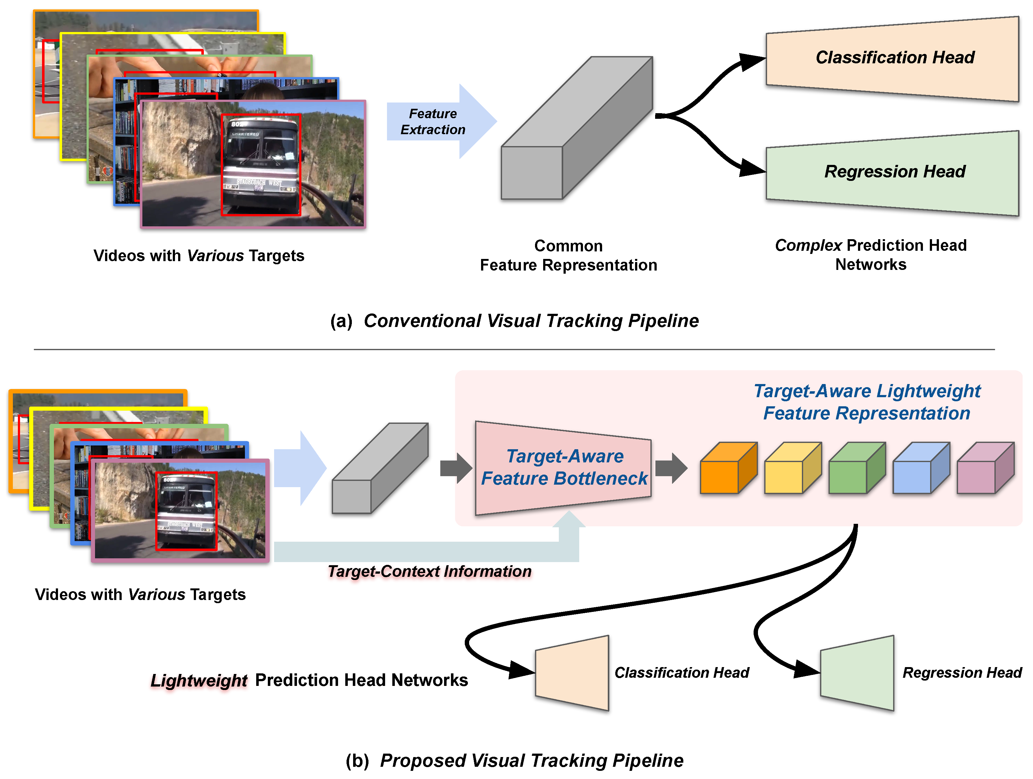
• In contrast to previous lightweight tracker design approaches where only backbone feature extractors are compressed without consideration of prediction heads, or require a specialized network structure for an architecture search, our feature bottleneck approach is more versatile in terms of backbone network selection and can reduce the computation of prediction heads.
• Under evaluation, we obtain comparable tracking accuracy metrics on multiple benchmarks for visual tracking, LaSOT and GOT-10k, using lighter backbone feature extractors, compared to the other heavier ResNet backbones used in [29].
• Owing to our proposed feature bottleneck module, we accomplish a real-time processing speed of 74 fps which is substantially faster than the sub-real-time speeds of previous global search-based, computationally heavier visual tracking algorithms.

2. Related Work

There has been an ongoing trend in the visual tracking literature to formulate the visual tracking task as a tracking-by-detection problem [30], which is to localize the target object inside a designated search area by performing a binary classification task. Trackers are formulated as classifier models where the model can classify the region of the target as a positive class and the region outside the target area as a negative class. At test time, the region score with the largest positive value is chosen as the predicted output region, where additional bounding box regression and refinement is possible as in the two-stage object detection literature [7].

CNN-based Trackers: Along with powerful feature representations brought by CNNs trained from classification tasks [6,31,32], visual tracking algorithms also make use of these representations. Notable examples include MDNet [33] and RT-MDNet [34] which uses a VGG [31] network with a binary multi-domain classifier on top. Employing correlation filters on pretrained representations has also gained attention where the aim of the filters is to produce a 2D Gaussian score map with the maximum score at the center position of the target region. Starting from the most notable KCF [35], further extensions have been proposed, such as using a hierarchical structure [36], joint group features [37], continuous correlation operators [38], and many more [39,40,41].

Siamese Network-based Trackers: Inspired by the simplicity and fast speed of these convolutional correlation filter-based formulations, SiamFC [9] aims to use Siamese networks to further make use of deep representations. Different from [42,43], SiamFC [9] has gained popularity owing to its fully convolutional architecture and simpler formulation compared to correlation filters. Given two image patches, where the target image patch is cropped from the initial frame using the initial target state, and the search image patch is cropped around the candidate region in a given video frame, target and search feature maps are extracted using a common backbone CNN feature extracting model. Afterward, a cross-correlation operation is performed between the feature maps to obtain a similarity value map where the location with the highest similarity value is picked as the predicted position. Many works improving the original SiamFC have been proposed, where deeper and wider backbones are employed [10,11], region proposal networks [7] are used [13,14], an additional branch for estimating the target center is added [15,16], and anchor-free formulation is used [44,45].

Transformer-based Trackers: With the recent advances in the transformer architecture [46] for the natural language processing (NLP) field, the application of attention-based modeling to computer vision research has gained popularity [8,47]. Starting with TransT [17] which substitutes the feature cross-correlation layer of the Siamese tracker with their proposed multi-head attention (MHA)-based feature fusion block, most transformer-based tracking algorithms have proposed modifications to the Siamese network architecture to replace the cross-correlation operation between target and search feature maps. Other approaches include STARK [18], CTT [48], and DTT [49] which employ encoder–decoder architecture. Recently, inspired by vision transformers (ViT) [8], joint feature extraction and correlation modeling with transformers have been proposed. Representative works include OSTrack [50], which uses one-stream framework using only MHA blocks, and SwinTrack [12], which uses the efficient Swin Transformer [51] architecture for feature extraction and fusion.

Lightweight Trackers: Due to the importance of a fast, real-time speed of visual tracking algorithms for practical applications, approaches aimed for designing lightweight and efficient networks for visual tracking have also gained attention. Approaches for reducing the computational load of neural networks in general [52] include weight quantization [23], pruning [24], architecture search [26], low-rank weight decomposition [53], and general model compression [54], where these line of works were successful for a dramatic reduction in the computational load of image classification networks. For visual tracking applications, there are approaches for adding a lightweight mixer network to the MobileNetV2 [55] backbone [56], a compact latent encoder for network adjustment [57], one-shot network architecture search [58], and using an efficient transformer architecture [59].

3. Proposed Method

In this section, we delineate the proposed target-aware feature bottleneck tracker (TAFT), where the overall tracking algorithm largely includes three stages: (1) the feature extraction and target-aware bottleneck stage, (2) a region proposal from the correlated feature maps, and (3) the region pooling and classification stage. In the following sections of this paper, we first illustrate an overview of our visual tracking algorithm. Then, we describe the details for each tracking stage, including tracking with our target-aware feature bottleneck module. Subsequently, we describe the training and implementation details with architectural details, training data, and hyperparameter values. Figure 2 illustrates the overview of the overall visual tracking algorithm.

3.1. Overview of the Baseline Tracking Algorithm

The first stage of the tracking algorithm involves feature extraction from input video frames. For input, a pair of RGB frame images $I_z,I_x\in {\mathbb{R}}^{H\times W\times 3}$ is given, where $I_z$ is the initial (query) frame image which includes the target object along with its initial state $b_0\in {\mathbb{R}}^4$ as the bounding box coordinates, and $I_z$ is the current frame image in which we aim to find the target object. The dimensions of the input images are identical, with spatial sizes of height H and width W with RGB channels. Feature representations are extracted by utilizing the backbone feature extraction net $\varphi (·)$, and feature representations for input images $I_z$ and $I_x$ are obtained as $F_z=\varphi \left(I_z\right),F_x=\varphi \left(I_x\right)\in {\mathbb{R}}^{h\times w\times c}$, respectively. The output feature maps hold spatial sizes of width w and height h, with c channels, where the pooling layer and kernel stride reduce the spatial size from the original $H\times W$. The backbone feature extractor $\varphi (·)$ can be any deep neural network pretrained with an image classification task, where the linear classifier layer is removed. For efficient training purposes, some of the last layers are chosen for finetuning, whereas other layers remain frozen. Additional technical details on the architecture, dimensions, hyperparameters, and training method are explained in Section 3.4.

After extracting the target and search feature maps $F_z,F_x\in {\mathbb{R}}^{h\times w\times c}$, the region proposal stage is conducted to search candidate areas that are similar to the target appearance, and these areas can be further classified and refined at the subsequent region classification stage. From the target feature map $F_z$, the initial bounding box coordinates $b_0$ can be used with the ROIAlign [60] operation to obtain spatially pooled target representation $z\in {\mathbb{R}}^{s\times s\times c}$. The $\mathtt{ROIAlign}(·)$ operation receives two inputs, which are the feature map and the bounding box coordinates. Then, the feature map is cropped based on the given bounding box coordinates and resized using linear interpolation to obtain a spatially pooled feature representation. We obtain the target representation as in $z=\mathtt{ROIAlign}(F_z,b_0)$, and s is predefined as the width and height dimension of the pooled target representation. Subsequently, a cross-correlation operation is performed in a depth-wise manner on the search feature map $F_x$ using target feature representation z as a kernel by

$$\widehat{x}=F_x\ast z,$$

(1)

in which ∗ represents the cross-correlation operation with a stride size of 1 and 0-padding size of $\lfloor \frac{s}{2}\rfloor$ in order to keep the spatial dimensions consistent. The output correlation feature map $\widehat{x}\in {\mathbb{R}}^{h\times w\times c}$ is passed onto the prediction heads for the region proposal net (RPN) operation, to produce two output prediction maps for the region proposal. Similar to the formulation in FCOS [61], the point-wise class label map $y_C\in {\mathbb{R}}^{h\times w\times 2}$ with the point-wise box estimation map $y_R\in {\mathbb{R}}^{h\times w\times 4}$ are predicted as below,

$$y_C=f_C^P\left(\widehat{x}\right),y_R=f_R^P\left(\widehat{x}\right),$$

(2)

where $f_C^P,f_R^P$ are RPN branches which consist of convolution, ReLU, and normalization [62] layers. Both output maps represent the point-wise class labels and bounding box coordinates, where the predicted point-wise class label map $y_C$ contains the binary logit values $y_C^{(i,j)}\in {\mathbb{R}}^2$ for a given row and column indices $(i,j)$, where the softmax probability of this point being inside or outside the target box region can be calculated for each position. For points $(i,j)$ inside the target box region, the predicted point-wise bounding box regression map $y_R$ represents the four corners of the estimated target bounding box where $y_R^{(i,j)}\in {\mathbb{R}}^4$ regresses the four boundaries, which are the top, bottom, left-, and right-side coordinates given the target box. Afterward, the non-maximum suppression (NMS) operation is performed on the bounding boxes with the highest probability scores to remove overlapping boxes that exceed a given threshold, where the top-N candidate ROI (region-of-interest) boxes $\{{\widehat{b}}_1,\dots ,{\widehat{b}}_N\}$ can be chosen for the subsequent region classification stage.

Given the top-N ROI boxes from the previous region proposal stage, we refine these predictions to choose a single output bounding box with the highest classification score. First, using the candidate boxes $\{{\widehat{b}}_1,\dots ,{\widehat{b}}_N\}$, the ROIAlign operation is performed as in $x_i=\mathtt{ROIAlign}(F_x,{\widehat{b}}_i),i\in \{1,\dots ,N\}$ where $x_i\in {\mathbb{R}}^{s\times s\times c}$ are the spatially pooled candidate feature representations with the same spatial and channel dimensions as the target feature representation z. Afterward, the candidate feature representations $x_i$ are cross-correlated with the target feature representation z as in

$${\widehat{x}}_i=x_i\otimes z,$$

(3)

where ⊗ is the element-wise product between two tensors of identical dimensions. Then, from the cross-correlated features ${\widehat{x}}_i\in {\mathbb{R}}^{s\times s\times c}$, the ROI class logits $y_{D,i}\in {\mathbb{R}}^2$ and box refinement values $y_{S,i}\in {\mathbb{R}}^4$ are obtained as in

$$y_{D,i}=f_D^Q\left({\widehat{x}}_i\right),y_{S,i}=f_S^Q\left({\widehat{x}}_i\right),$$

(4)

where the branches $f_D^Q,f_S^Q$ also consist of convolution, ReLU, and normalization [62] layers. The output class logits are concatenated to summarize the classification scores $y_D={[y_{D,1},\dots ,y_{D,N}]}^T\in {\mathbb{R}}^{N\times 2}$ to represent all binary logits for the ROIs, where the softmax operation is performed to obtain positive class probabilities and the k-th ROI ${\widehat{b}}_k\in {\mathbb{R}}^4$ with the maximum probability chosen for further bounding box refinement. Given the ROI ${\widehat{b}}_k={[x_k^c,y_k^c,w_k,h_k]}^T$, where $x_k^c,y_k^c\in \mathbb{R}$ are the horizontal and vertical center coordinates of the box, and $w_k,h_k\in \mathbb{R}$ are the width and height of the box, respectively, these values are refined using the refinement values $y_{S,k}={[d{x}_k,d{y}_k,d{w}_k,d{h}_k]}^T\in {\mathbb{R}}^4$ as in

$$\begin{array}{c}\hfill {x_k^c}^{\prime }=x_k^c+w_k·dx,{y_k^c}^{\prime }=y_k^c+h_k·dy,\\ \hfill w_k^{\prime }=w_k·exp\left(dw\right),h_k^{\prime }=h_k·exp\left(dh\right),\end{array}$$

(5)

to produce a refined ROI of ${{\widehat{b}}_k}^{\prime }={[{x_k^c}^{\prime },{y_k^c}^{\prime },{w_k}^{\prime },{h_k}^{\prime }]}^T$ which serves as the output of the tracker for a given frame.

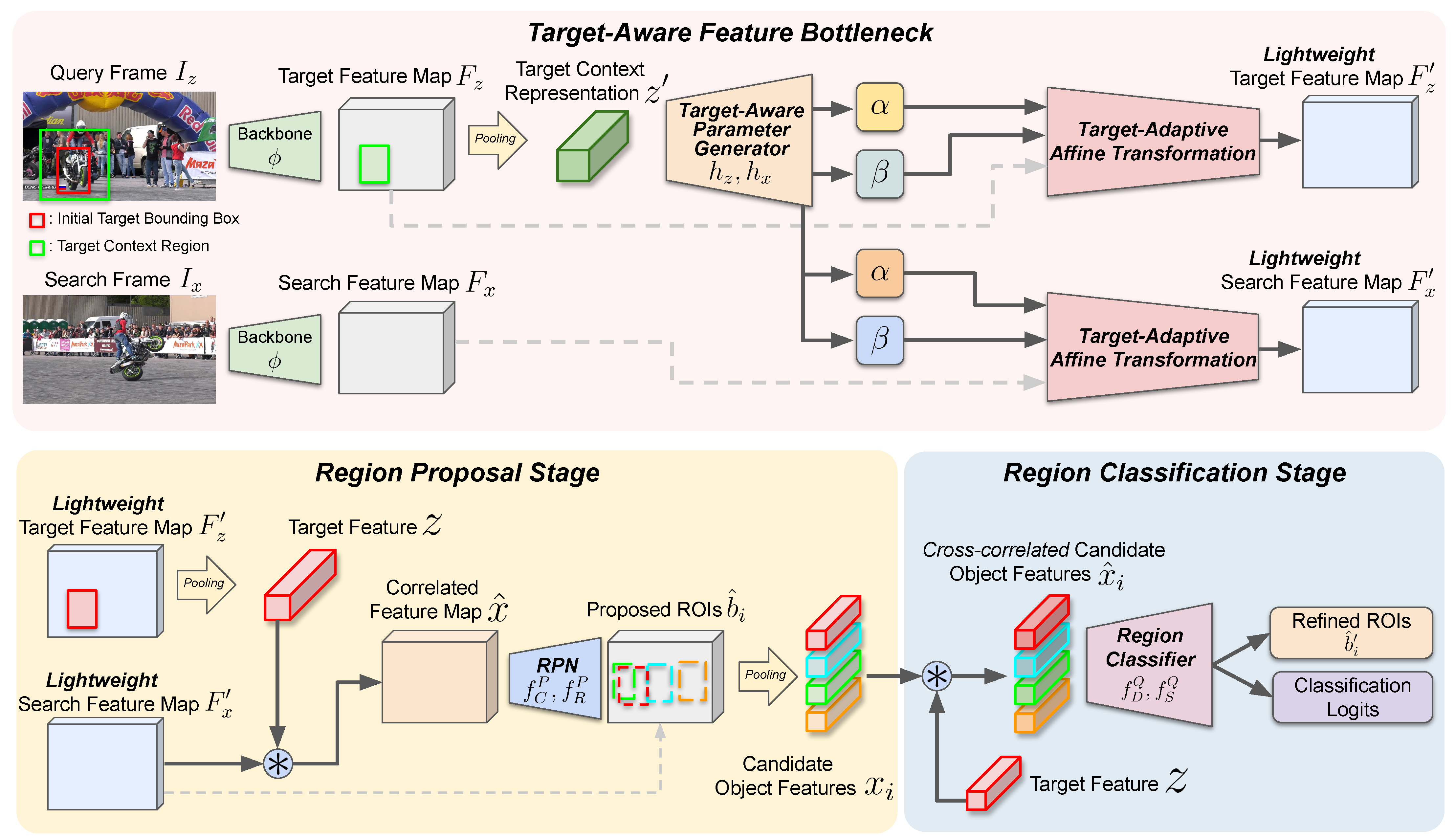
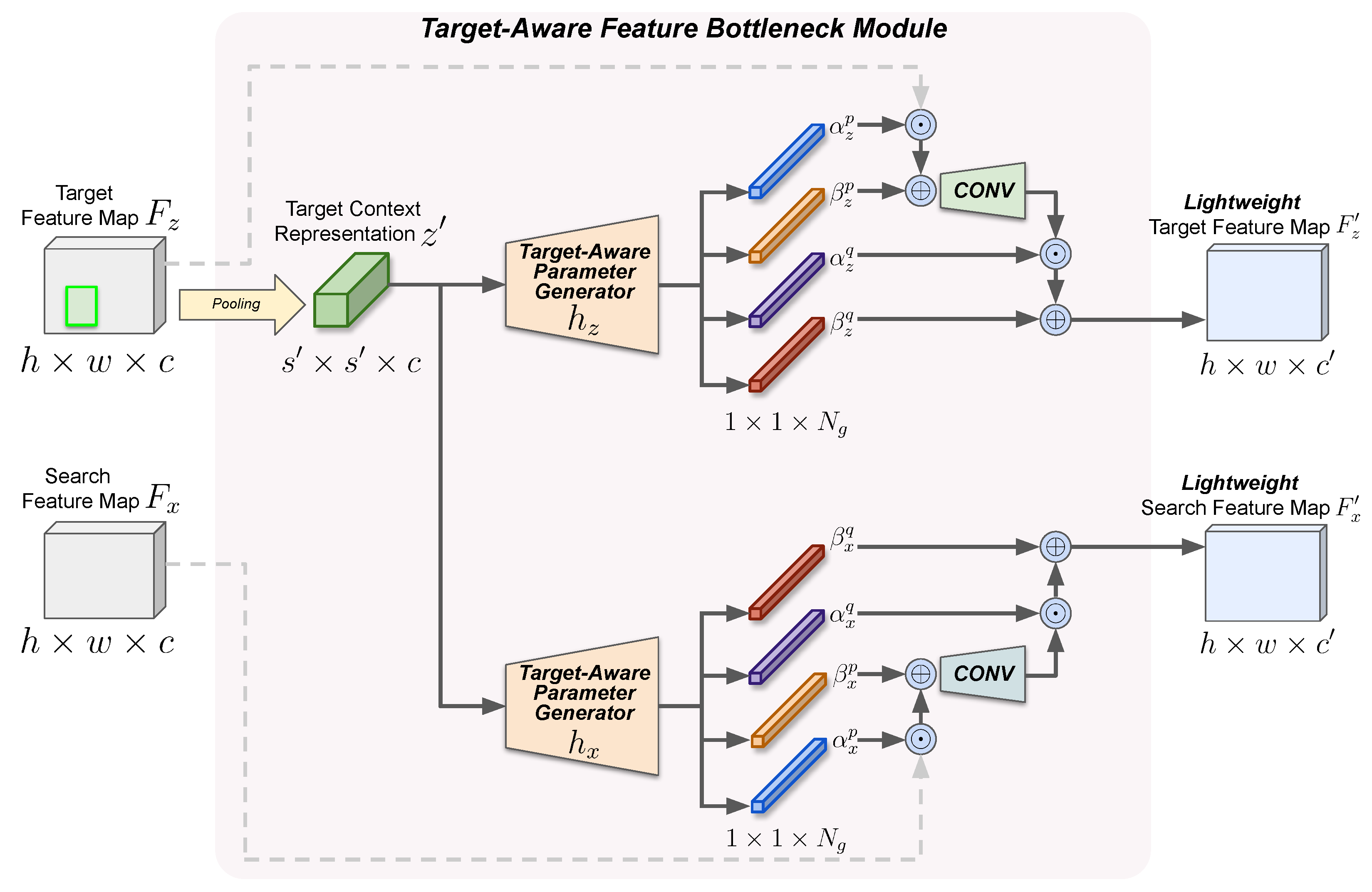
3.2. Incorporation of the Target-Aware Feature Bottleneck Module

In this section, we describe the detailed operation for our proposed target-aware feature bottleneck module. Our goal is to reduce the channel dimension of the backbone feature representation for efficient and fast subsequent computation, with minimal trade-off in discriminative performance. At the high level, our target-aware feature bottleneck module (TAFM) operates as in

$${F_z}^{\prime },{F_x}^{\prime }=\mathtt{TAFM}(F_z,F_x,b_0),$$

(6)

where the output feature maps are ${F_z}^{\prime },{F_x}^{\prime }\in {\mathbb{R}}^{h\times w\times c^{\prime }}$ and the hyperparameter $c^{\prime }<c$ is chosen for reduced computation. Using lightweight target and search feature maps ${F_z}^{\prime },{F_x}^{\prime }$, the subsequent region proposal (Equation (2)) and classification and refinement (Equation (4)) can be performed with less FLOPs operation, and the amount of reduced computation can vary depending on the architecture of the prediction heads. Our target-aware bottleneck module processes feature maps $F_z,F_x$ through three stages, which are the (1) pre-modulation stage, (2) convolution stage, and (3) post-modulation stage. The convolution stage performs a simple point-wise conv operation which reduces the channel size from c to $c^{\prime }$, whereas the pre- and post-modulation stages perform channel-wise feature modulation through affine transformation based on the target-aware information extracted from the target feature representation.

First, we start from extracting the target-specific information to obtain target-adaptive parameters for feature modulation. To extract the target-specific information, we use the target feature map $F_z$ obtained from the initial frame image $I_z$ and the initial target bounding box $b_0={[x_0^c,y_0^c,w_0,h_0]}^T$ with the box center coordinates $(x_0^c,y_0^c)$, width $w_0$, and height $h_0$. We obtain a spatially pooled target context representation $z^{\prime }\in {\mathbb{R}}^{s^{\prime }\times s^{\prime }\times c}$ as in

$$z^{\prime }=\mathtt{ROIAlign}(F_z,{b_0}^{\prime }),$$

(7)

where ${b_0}^{\prime }$ is the dilated initial target bounding box ${b_0}^{\prime }={[x_0^c,y_0^c,{\gamma }_c{w}_0,{\gamma }_c{h}_0]}^T$, and ${\gamma }_c\ge 1$ is the hyperparameter for controlling the amount of context information to be included around the target object.

Subsequently, from the pooled feature map $z^{\prime }$, the feature modulation parameters for target-adaptive affine transformation are obtained using the target-aware parameter generator as in

$$\begin{array}{cc}\hfill {\alpha }_z^p,{\beta }_z^p,{\alpha }_z^q,{\beta }_z^q& =h_z\left(z^{\prime }\right)\hfill \\ \hfill {\alpha }_x^p,{\beta }_x^p,{\alpha }_x^q,{\beta }_x^q& =h_x\left(z^{\prime }\right),\hfill \end{array}$$

(8)

where all the output parameters are ${\alpha }_z^p,{\beta }_z^p,{\alpha }_z^q,{\beta }_z^q,{\alpha }_x^p,{\beta }_x^p,{\alpha }_x^q,{\beta }_x^q\in {\mathbb{R}}^{N_g}$, and $N_g$ is a hyperparameter for the number of feature groups. The output parameters are used for affine transformation where ${\alpha }_{·}^{·}$ are later used as multipliers, and ${\beta }_{·}^{·}$ are used as biases. The parameters with superscript p are used in the pre-modulation stage and with superscript q are used in the post-modulation stage, and the parameters with subscript z are used to modulate the target feature map $F_z$ and with subscript x are used to modulate the search feature map $F_x$. For our experiments, we choose the number of feature groups $N_g\ll c^{\prime }<c$ for a reduced number of weights and increased efficiency, where group-wise modulation provides an adequate trade-off between performance and efficiency. For $h_z$ and $h_x$, we use a differentiable, lightweight neural network composed of convolution, global average pooling, and linear layers with ReLU in between, where all the layers except for the last layer are shared between networks $h_z$ and $h_x$. Using the output parameters from $h_z$ and $h_x$, the input feature maps $F_z$ and $F_x$ go through the three aforementioned stages as in

$$\begin{array}{cc}\hfill {F_z}^{\prime }& ={\alpha }_z^q\odot \sigma ({\alpha }_z^p\odot F_z\oplus {\beta }_z^p)\oplus {\beta }_z^q\hfill \\ \hfill {F_x}^{\prime }& ={\alpha }_x^q\odot \sigma ({\alpha }_x^p\odot F_x\oplus {\beta }_x^p)\oplus {\beta }_x^q,\hfill \end{array}$$

(9)

where $\sigma (·)$ represents a $1\times 1$ convolution layer with unit stride, and ⊙ and ⊕ are group-wise multiplication and addition operators that appropriately broadcast the parameters to the channels of each group. Because the affine transformation parameters are obtained conditioned on the target context feature, the tracker can adaptively change these parameters according to the given scene, where the tracker can keep its discriminative capacity even under high compression. Please refer to Figure 3 for an overall view of the framework and operation of the target-aware bottleneck and Algorithm 1 for the step-by-step operation of our proposed tracker with the integrated target-adaptive feature bottleneck module.    

Algorithm 1 Visual tracking with target-aware feature bottleneck

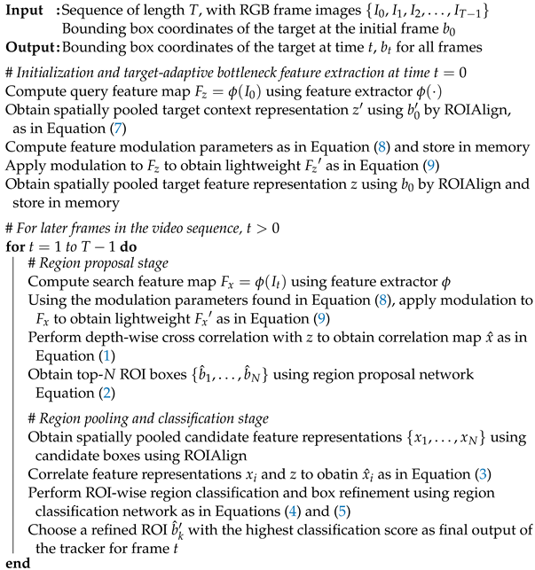
3.3. Training the Proposed Framework

Herein, we provide the details that are relevant to training our overall tracking framework, where we describe the loss functions and optimization method that are used for training the overall tracking model. We apply loss functions on the outputs of the RPN and the region classifier net, where the target-adaptive feature bottleneck module is iteratively optimized from the transferred gradients obtained by optimizing the subsequent prediction head networks.

To train the region proposal network with two branches shown in Section 3.1, we enforce loss functions on the outputs of both branches $f_C^p,f_R^p$, which are $y_C\in {\mathbb{R}}^{h\times w\times 2},y_R\in {\mathbb{R}}^{h\times w\times 4}$ as in

$$L^P(\{y_C,y_C^{\ast }\},\{y_R,y_R^{\ast }\})=\frac{1}{hw}\sum _{i,j}{L}_C^P(y_C^{(i,j)},y_C^{\ast (i,j)})+\frac{{\lambda }_P}{N_P}{\mathbf{1}}_{\{y_C^{\ast (i,j)}>0\}}\sum _{i,j}{L}_R^P(y_R^{(i,j)},y_R^{\ast (i,j)})$$

(10)

where the superscript $(i,j)$ denotes a spatial position in the output maps; $y_C^{\ast },y_R^{\ast }$ denote corresponding ground truth maps; and $N_P$ is the number of positions in the ground truth classification map $y_C^{\ast }$ with positive labels $y_C^{\ast (i,j)}>0$. For the output of classification branch $y_C$, focal loss [63] is used to compensate for class imbalance, where $L_C^P$ is applied on all locations $(i,j)$ in the output as in

$$L_C^P(y_C^{(i,j)},y_C^{\ast (i,j)})=-(1-y_C^{\ast (i,j)})y_C^{(i,j)\gamma }log(1-y_C^{(i,j)})-y_C^{\ast (i,j)}{(1-y_C^{(i,j)})}^{\gamma }log\left(y_C^{(i,j)}\right),$$

(11)

in which $\gamma$ is a focus hyperparameter for controlling the importance between easy and hard targets. For the output of the regression branch $y_R$, the loss is only enforced on locations in the positive region ($y_C^{\ast (i,j)}>0$) where our goal is to maximize the intersection-over-union (IoU) overlap between the ground truth and predicted bounding boxes as in

$$L_R^P(y_R^{(i,j)},y_R^{\ast (i,j)})=1-\frac{|b_R^{(i,j)}\cap b_R^{\ast (i,j)}|}{|b_R^{(i,j)}\cup b_R^{\ast (i,j)}|},$$

(12)

where $b_R^{(i,j)},b_R^{\ast (i,j)}$ denote the predicted bounding box and ground truth bounding box made from the values $y_R^{(i,j)},y_R^{\ast (i,j)}\in {\mathbb{R}}^4$, respectively. $|·|$ denotes the total area size of a given region, ∩ represents the overlap operation (intersection) between two regions, and ∪ is the union operation over two regions.

From the region proposals generated by the region proposal network, candidate features are spatially pooled and correlated with the target feature representation and fed to the region classification branches $f_D^Q,f_S^Q$, where the loss is enforced on the outputs $y_D\in {\mathbb{R}}^{N\times 2}$ and $y_S\in {\mathbb{R}}^{N\times 4}$ as in

$$L^Q(\{y_D,y_D^{\ast }\},\{y_S,y_S^{\ast }\})=\frac{1}{N}\sum _i{L}_D^Q(y_D^i,y_D^{\ast i})+\frac{{\lambda }_Q}{N_Q}{\mathbf{1}}_{\{y_D^{\ast i}>1\}}\sum _i{L}_S^Q(y_S^i,y_S^{\ast i}),$$

(13)

where i indicates the index of a candidate ROI; $y_D^{\ast },y_S^{\ast }$ denote the corresponding ground truth labels; and $N_Q$ denotes the quantity of ROI regions that are positively labeled $y_D^{\ast i}>1$. The ground truth classification label $y_D^{\ast i}$ is determined by the IoU value of the RoI where $y_D^{\ast i}=1$ is assigned to RoIs exceeding a threshold value ${\tau }_p=0.5$, and $y_D^{\ast i}=0$ is assigned to RoIs below a threshold value ${\tau }_n=0.4$. For the output of the classification branch $y_D$, focal loss is also used as in Equation (11) where the same $\gamma$ is used. For the output of the bounding box refinement branch $y_S$, $L_1$ loss is enforced as in

$$L_S^Q(y_S^i,y_S^{\ast i})=\left|\right|y_S^i-y_S^{\ast i}{\left|\right|}_1,$$

(14)

which is a standard $L_1$ distance between two vectors, to minimize the distances for four corners of the bounding box coordinates.

Additionally, because an unconstrained target-aware feature bottleneck module can generate affine transformation parameters that are too large or too small, especially for the multipliers ${\alpha }_{·}^{·}$, this can cause overfitting to the training examples and hamper generalization due to a large distribution shift in the intermediate activation values. To prevent this phenomenon, we enforce an additional regularization term along with the standard $L_2$ weight decay term as in

$$L^R(\mathit{\theta },\mathit{\alpha })={\lambda }_R{\left|\right|\mathit{\theta }\left|\right|}_2+{\lambda }_{\alpha }\left|\right|\mathit{\alpha }-{\mathbf{1}\left|\right|}_1,$$

(15)

where $\mathit{\alpha }=[{\alpha }_z^p,{\alpha }_z^q,{\alpha }_x^p,{\alpha }_x^q]\in {\mathbb{R}}^{4N_g}$, ${\lambda }_R$ is the weight decay hyperparameter, and ${\lambda }_{\alpha }$ is the loss balancing hyperparameter. The first term is for the standard $L_2$ weight decay enforced on all weights $\mathit{\theta }$ of the neural network, and the second term is an $L_1$ distance term enforced on all multipliers ${\alpha }_{·}^{·}$ encouraging them not to deviate too far from 1, in order to prevent overfitting due to excessively large or small parameters.

Employing the loss functions as shown above, we can formulate the total loss function $L^T$, which is the final target for optimization, as in

$$\begin{array}{cc}\hfill L^T(\{y_C,y_C^{\ast }\},& \{y_R,y_R^{\ast }\},\{y_D,y_D^{\ast }\},\{y_S,y_S^{\ast }\})\hfill \\ \hfill & =L^P(\{y_C,y_C^{\ast }\},\{y_R,y_R^{\ast }\})+{\lambda }_T{L}^Q(\{y_D,y_D^{\ast }\},\{y_S,y_S^{\ast }\})+L^R(\mathit{\theta },\mathit{\alpha }),\hfill \end{array}$$

(16)

where ${\lambda }_T$ is the loss balancing hyperparameter. In the early stage of the training phase, we use ${\lambda }_T=0$ to train the region proposal network first and switch to ${\lambda }_T=1$ after an epoch of training. This stabilizes the training because the quality of the candidate ROI boxes from the region proposal network are low in the early stage, and this imbalance enforces a negative bias on the subsequent region classification network. After this burn-in phase, the total loss function can be optimized by employing the SGD-based optimizer where we use the Adam optimizer [64] in our experiments.

3.4. Implementation Details

In this section, we describe additional training details on the training and implementation of our proposed algorithm, where we clarify the training datasets, hyperparameter selections, and further architectural specifications. For the training datasets, we employ training splits of the LaSOT [19], GOT-10k [20], ImageNetVID [65], and YoutubeBB [66] video datasets, where we use a subset of held-out sequences from the LaSOT benchmark as the validation split. To sample a training image pair of query and search frames, we randomly choose a video sequence from a large-scale video dataset where an individual sequence is sampled from a uniform distribution. For a sampled image pair $(I_z,I_x)$ where all values are normalized to the range $[0,1]$, random data augmentation of additive Gaussian noise ($\sigma =0.05$), color jittering ($\sigma =0.025$), Gaussian blur (random kernel size of $\{3,5,7,9\}$), and horizontal flip are performed with an individual probability of $p=0.2$ for improved generalization capabilities. After the data augmentation, channel-wise normalization is performed on the input frames using the identical scheme used in ResNet [6], where the mean $\mu =[0.485,0.456,0.406]$ and standard deviation $\sigma =[0.229,0.224,0.225]$ are used as in $(I-\mu )/\sigma$. To extract feature representation from the input frames, we employ ResNet-18 [6] for the feature extractor backbone $\varphi (·)$ because it requires relatively less computation compared to other trackers with heavier backbones [10,11,18] while achieving moderate performance on various downstream tasks. The input frames are resized to $W=666,H=400$ and are fed to $\varphi (·)$ while retaining the original aspect ratio where the longest edge of the input image is matched with the output height/width, and zero padding is applied to the right or bottom side of the shorter edge. The output feature maps from $\varphi (·)$ have dimensions of $h=25,w=42,c=512$, where their channel dimensions are reduced to $c^{\prime }$ to produce lightweight feature maps.

From the feature maps, a pooled target feature $z^{\prime }$ with a spatial dimension of $s=5$ is obtained, and the correlated feature map $\widehat{x}$ is processed through the region proposal network branches $f_C^P,f_R^P$, where they both consist of two $3\times 3$ convolution layers and a final $1\times 1$ convolution layer with ReLU nonlinearity and group normalization [62] layers with the group number $G=16$ in between. The channel dimension of the intermediate representations are kept to $c^{\prime }$. With our proposed feature bottleneck module, the number of channels reduces from $c=512$ to $c^{\prime }$, where $c^{\prime }$ can vary between different settings, and we test our method using the values $c^{\prime }\in \{256,128,64\}$, each corresponding to a computational reduction rate of $\frac{1}{2},\frac{1}{4},\frac{1}{8}$. We obtain the total of the top-$N=64$ candidate ROI boxes by applying NMS with a threshold of $0.9$ and spatially pool the ROI features with a spatial dimension of $s=5$. Afterward, the region classification network branches $f_D^Q,f_S^Q$ process the correlated candidate feature representations, where both branches also consist of two $3\times 3$ convolution layers and a final $1\times 1$ convolution layer with ReLU nonlinearity and group normalization layers with a group number $G=16$ in between.

Regarding our target-aware feature bottleneck module, it operates on the target context representation $z^{\prime }$ which is pooled using a dilated initial target bounding box with a context hyperparameter of ${\gamma }_c=2$ and feature representation with a spatial size of $s^{\prime }=9$. The input is processed using network branches $h_z,h_x$ where they share two convolution layers with ReLU and group normalization layers, with a channel compression rate of 4 when processing the intermediate representations. Afterward, global average pooling is performed on the shared intermediate representation, and modulation parameters ${\alpha }_z^p,{\beta }_z^p,{\alpha }_z^q,{\beta }_z^q,{\alpha }_x^p,{\beta }_x^p,{\alpha }_x^q,{\beta }_x^q\in {\mathbb{R}}^{N_g}$ are obtained using a single linear projection layer. We test with different feature group number hyperparameters $N_g\in \{32,16,4\}$ to find a balance between efficiency and performance. At the training stage, because starting from affine transformation multipliers ${\alpha }_{·}^{·}$ that are initialized to near 0 can cause instability and inefficient training, we formulate the prediction of ${\alpha }_{·}^{·}$ as in

$${\alpha }_{·}^{·}=1+{\tilde{\alpha }}_{·}^{·},$$

(17)

where the network branches $h_z,h_x$ predict ${\tilde{\alpha }}_{·}^{·}$ instead of directly predicting ${\alpha }_{·}^{·}$. This stabilizes the training process, achieves faster convergence, and can encourage the target-aware feature bottleneck module to reuse useful feature representations from the original input feature map.

To train the overall framework and perform optimization of the total loss function in Equation (16), we use the Adam [64] optimizer where the size of a single batch is 16 image pairs for each update. We use a learning rate of ${10}^{-4}$ and it is kept the same throughout the entire training process, and the $L_2$ weight decay hyperparameter is set to ${\lambda }^R={10}^{-5}$. Other loss balancing terms ${\lambda }_P,{\lambda }_Q,{\lambda }_T,{\lambda }_{\alpha }$ are all set to 1, and we use the focal loss hyperparameter $\gamma =2$. We set $c^{\prime }=128$ and $N_g=16$ as the default settings for our tracker. We initialize the feature extractor $\varphi (·)$ with the weights of ResNet-18 and freeze the residual blocks with the exception of the last residual module, in which the stride size is changed from 2 to 1 and the output feature map has a larger spatial resolution. To implement our algorithm, we use Python 3.6 with PyTorch [67] v1.10.2 installed on an Ubuntu 20.04 environment. We train and evaluate the run-time measurements of our model on a single NVIDIA RTX 4090 GPU with 48 GB of video memory with an i9-12900K CPU with 128 GB of memory.

4. Experiments

We present the experimental results in this section, where we test our algorithm on the large-scale benchmarks of LaSOT [19] and GOT-10k [20], representative of the performance evaluations on long-term and short-term videos, respectively. Quantitative evaluations are conducted where the proposed tracker is compared with other recently proposed trackers, and we conduct ablation experiments with different settings for feature bottleneck hyperparameters, with an attribute-wise ablation analysis of the LaSOT test set. Additionally, we provide qualitative results and a comparison to further visualize the effectiveness of our proposed method.

4.1. Experimental Settings

For the experiments, we run our tracking algorithm given the testing split of two benchmark datasets and obtain performance metrics to conduct comparisons with other trackers. When evaluating a performance metric, we use a fixed hyperparameter setting throughout all the sequences in the test split. The large-scale LaSOT [19] benchmark represents a long-term tracking benchmark where it contains mostly long sequences with an average length of 2512 frames, which is equivalent to $83.7$ s under a 30 fps setting. It contains 1400 sequences with 70 target object categories, where 280 sequences are used for testing and the remaining sequences are used for training. Along with the bounding box coordinates, annotations of various challenge attributes such as occlusion, out-of-frame disappearances, motion blur, background clutter, etc., are provided. To evaluate a tracker, three performance metrics are used which are the area under the curve (AUC) of the output success plot, center pixel precision plot, and target-scale normalized pixel precision plot. Success plots and precision plots are generated by varying the threshold values of the IoU and center pixel error.

The large-scale GOT-10k [20] benchmark represents a short-term tracking benchmark where it contains mostly short-term sequences with an average length of 150 frames, which is equivalent to 15 s under a 10 fps setting as stated in the specifications [20]. It contains 10,000 sequences with 563 target object categories, where 180 representative test sequences were chosen for online evaluation. Different from previous benchmarks, GOT-10k aims to evaluate the tracker’s generalization performance under a one-shot protocol where the training and test splits have no overlap in the target object categories. For the evaluation metrics, the average overlap (AO) measure for the predicted output and the labeled GT are measured over the test sequences, and the success ratio (SR) using both IoU threshold values 0.50 and 0.75 is measured. We evaluate the trackers using the one-pass evaluation (OPE) setting.

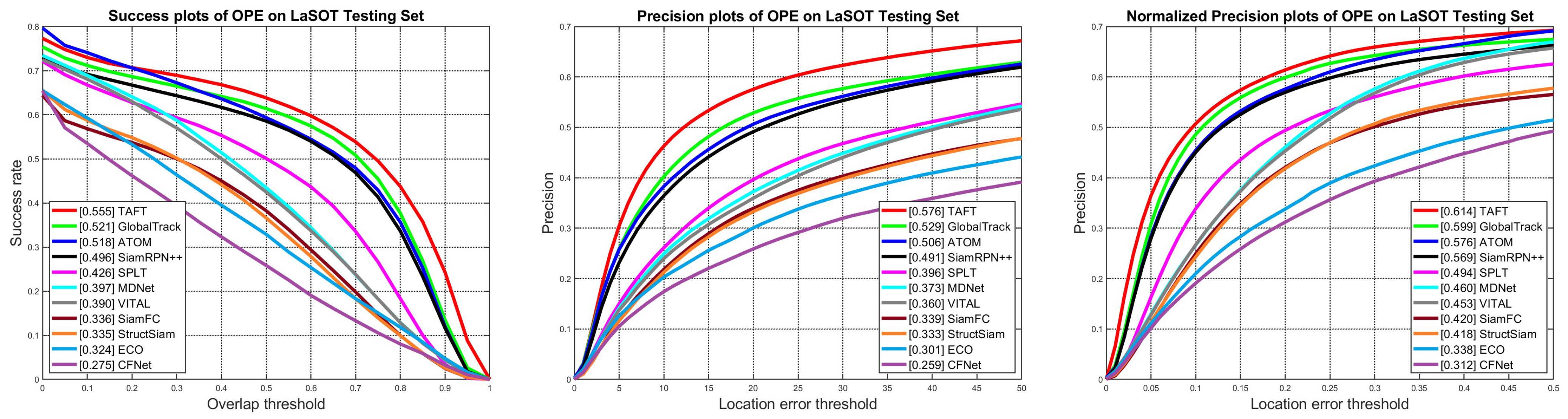
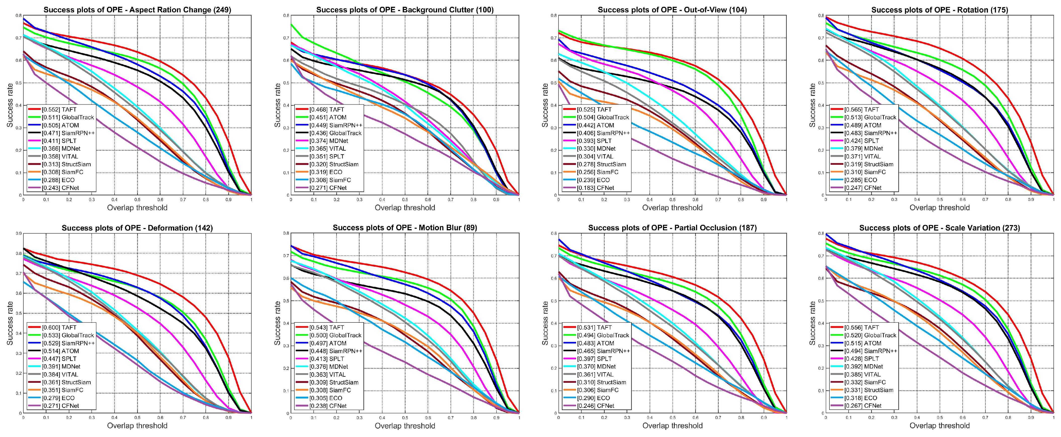
4.2. Quantitative Evaluation

We conduct evaluations for the proposed tracker given the testing splits of the LaSOT and GOT-10k benchmarks, and

Table 1. Quantitative evaluation on the test set of LaSOT.

	TAFT	GlobalTrack [29]	DiMP-50 [70]	ATOM [68]	DASiam [14]	SiamRPN++ [10]	MDNet [33]	SPLT [69]	Ocean [44]	CFNet [40]	SiamFC [9]	AutoMatch [71]	MCAGSA [72]	TFN [73]
AUC	0.555	0.521	0.569	0.518	0.448	0.496	0.397	0.426	0.560	0.275	0.336	0.583	0.572	0.528
Precision	0.576	0.529	-	0.506	0.427	0.491	0.373	0.396	0.566	0.259	0.339	0.599	-	0.527
Norm. Prec.	0.614	0.599	0.650	0.576	-	0.569	0.460	0.494	-	0.312	0.420	-	-	0.606
FPS	74	6	43	30	110	35	0.9	25.7	25	43	58	50	40	45

and

Table 2. Quantitative evaluation on the test set of GOT-10k.

(%)	TAFT	DiMP-50 [70]	ATOM [68]	SiamMask [22]	Ocean [44]	CFNet [40]	GOTURN [42]	SiamFC [9]	CCOT [38]	ECO [74]	CF2 [36]	MDNet [33]	TFN [73]
${\mathbf{SR}}_{\mathbf{0}.\mathbf{50}}$	65.2	71.7	63.4	58.7	72.1	40.4	37.5	35.3	32.8	30.9	29.7	30.3	0.683
${\mathbf{SR}}_{\mathbf{0}.\mathbf{75}}$	50.6	49.2	40.2	36.6	-	14.4	12.4	9.8	10.7	11.1	8.8	9.9	0.457
$\mathbf{AO}$	57.5	61.1	55.6	51.4	61.1	37.4	34.7	34.8	32.5	31.6	31.5	29.9	0.582

show the comparisons for the respective benchmarks. We name our algorithm, the target-adaptive feature bottleneck tracker, as TAFT in the subsequent tables and figures. From the performance metrics in Table 1, we observe that the proposed algorithm outperforms other ResNet-based trackers, such as GlobalTrack [29], ATOM [68], SPLT [69], and SiamRPN++ [10], and shows competitive performance compared to DiMP-50 [70] and Ocean [44]. Because the majority of these ResNet-based trackers are based on the ResNet-50 backbone, which is a much heavier network compared to the ResNet-18 backbone used in our tracker, our tracker runs at a much faster speed of 74 fps, thanks to the lighter backbone network and our proposed feature bottleneck module. Additional figures with comparisons for the success, precision, and normalized precision plots with varying overlap and location error threshold values are also shown in Figure 4.

The results for the test split of GOT-10k are shown in Table 2 where all the quantitative metrics are obtained by uploading the outputs for the test sequences to the authors’ online evaluation server (http://got-10k.aitestunion.com (accessed on 8 September 2023)). Our proposed TAFT also shows competitive performance compared to other trackers on the task of relatively short-term sequences, even though our baseline tracker GlobalTrack [29] is a long-term oriented global search-based tracker. Although every other tracker requires meticulous tuning for the hyperparameters regarding temporal smoothness, motion priors, and cosine window weighting, our proposed TAFT does not employ any of these motion priors and thus performs generally well on a wide variety of tracking scenarios. Additionally, because removing the motion prior also removes the dependency between consecutive frames, our tracker can be executed in a batch-wise fashion where multiple frames can be processed at once, enabling further acceleration of the tracking speed.

Ablation Study

To provide a further comprehensive analysis of our TAFT algorithm and our target-aware feature bottleneck module, we perform an ablation analysis of the various challenge attributes for visual tracking and test our module with multiple combinations of the feature channels numbers $c^{\prime }$ and the number of feature groups $N_g$. For the ablation study, we use the success plots acquired from the LaSOT test split and use the AUC measures for the evaluation and comparison.

Ablations on Challenge Attributes: To measure the robustness of TAFT on diverse challenge attributes in the tracking task, we visualize and compare the success plots of sequences with eight chosen attributes for the test split of LaSOT in Figure 5. Each test sequence is annotated with one or more challenge attributes, and the number of test sequences annotated with a given challenge attribute is denoted at the top of each plot. Our proposed TAFT achieves notable performance on the eight attributes, and the largest performance gains are obtained for the attributes of rotation, deformation, motion blur, and aspect ratio change. Owing to the target-specific information obtained from the initial frame, our proposed bottleneck module can fully utilize the target-context information and can learn to modulate the relevant channels that can be useful for localizing the target object under these attributes. Additionally, because the baseline tracker GlobalTrack is a motion prior-free global search-based tracking algorithm, it shows weaknesses under the attribute of background clutter when compared to SiamRPN++ and ATOM, where GlobalTrack is more likely to mislabel a similar distractor object in the background as a false positive. Although our tracker TAFT has the same global search-based framework, it achieves higher performance while running at a faster, real-time tracking speed.

Ablations on the Target-Aware Feature Bottleneck Module: To accurately quantify the effectiveness of the proposed module, we conduct a further ablation analysis for the proposed module and report the AUC metrics of the success plots obtained from the test split of the LaSOT dataset. First, we test our module with six different hyperparameter combinations of the output feature channel numbers $c^{\prime }$ and feature group numbers $N_g$ where we show the results in

Table 3. Ablation analysis of the target-aware feature bottleneck module.

Setting	${\mathit{c}}^{\prime }$	${\mathit{N}}_{\mathit{g}}$	${\mathit{c}}^{\prime }/\mathit{c}$	AUC
(1)	256	16	1/2	0.555
(2)	256	8	1/2	0.549
(3)	128	16	1/4	0.546
(4)	128	4	1/4	0.538
(5)	64	32	1/8	0.543
(6)	64	4	1/8	0.519
(7)	256	-	1/2	0.532

. We denote the reduction in the computational load of the prediction head as $c^{\prime }/c$, because the computational load is linearly proportional to the number of channels. Setting (1) in the first row is identical to the tracker used to report the performances in Table 1 and Table 2. If we reduce the number of feature groups $N_g$ to eight in setting (2), we observe a performance decrease of $-0.006$. For settings (3) and (4), we use $c^{\prime }=128$ with a varying number of $N_g$ and observe a similar trend where the performance decreases by $-0.008$ when $N_g$ is reduced. The same tendency can be observed in settings (5) and (6) where the channel number is further reduced to $c^{\prime }=64$, and reducing $N_g$ causes a significant decrease in performance by $-0.024$. From the results in settings (1)–(6), we can speculate that our target-aware feature modulation scheme plays a significant role in improving the target discriminability when tracking, and decreasing the feature group $N_g$ hampers the ability of fine-grained feature modulation of the bottleneck module. Additionally, to quantify the contribution of our proposed bottleneck module, we remove our module entirely in setting (7), where removing the module results in a performance decrease of $-0.023$, validating the effectiveness of our proposed framework for visual tracking.

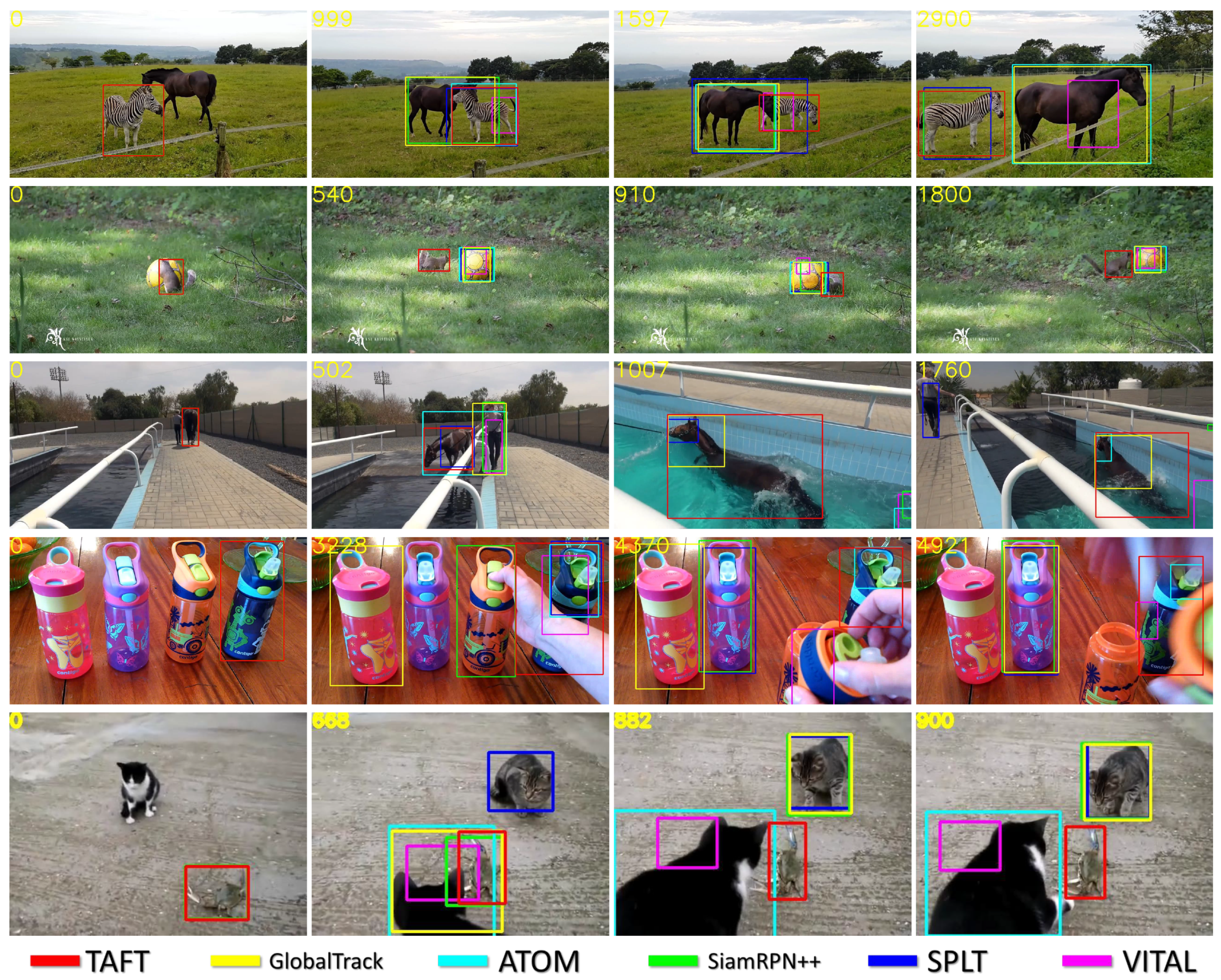
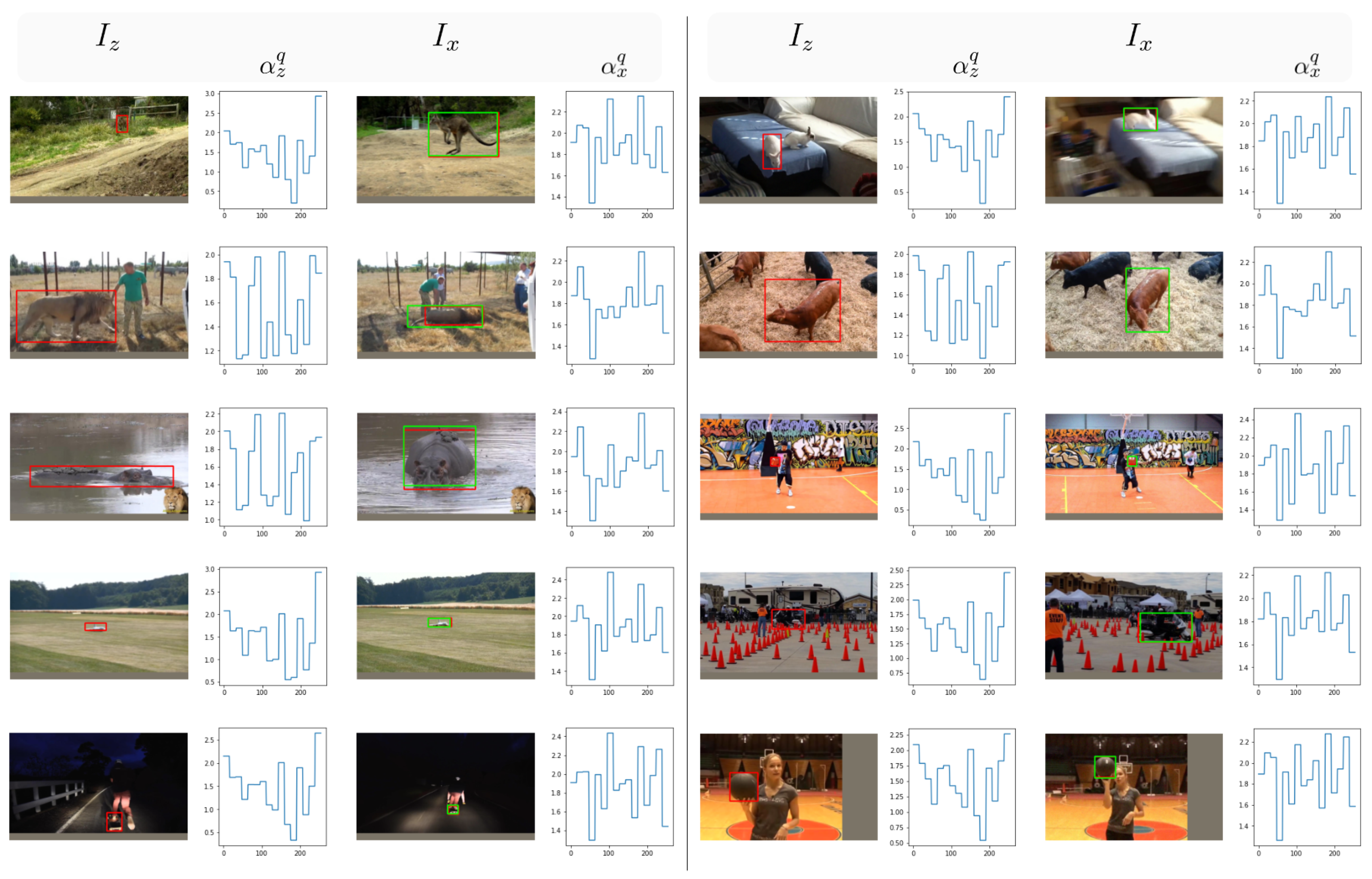
4.3. Qualitative Evaluations and Analysis

In this section, we provide further visualizations of the qualitative results produced by TAFT, on the test split of LaSOT. We show the bounding box output comparisons with other tracking algorithms in Figure 6, where we show the output of our tracker with ATOM, GlobalTrack, SPLT, SiamRPN++, and VITAL. The results from five example videos, zebra-17, squirrel-13, horse-15, bottle-14, and crab-3, are shown in each row, where the output bounding boxes for each tracker can be distinguished by its respective color shown in the bottom of the figure. While other tracking algorithms suffer from the drift issue arising from the challenges of distractor objects of a similar appearance and category as in zebra-17 and bottle-14, occlusion from other objects as in squirrel-13 and crab-3, and the deformation of the target as in horse-15, our proposed TAFT can successfully track the target object under these challenging circumstances.

Furthermore, we present additional visualizations for the target-adaptive feature modulation parameters in Figure 7, where group-wise multiplier values ${\alpha }_z^q$ and ${\alpha }_x^q$, which are applied to the feature groups as in Equation (9), are shown on ten example frame image pairs $(I_z,I_x)$ under the network hyperparameter setting (1) in Table 3. We observe that multiplier values can change adaptively given the target and its surroundings, and our target-aware feature bottleneck module is trained to utilize different feature groups in the lightweight search feature map ${F_x}^{\prime }$ and the query feature map ${F_z}^{\prime }$. Output multiplier values vary greatly between channel groups, based on the factor of the query or search patch, target object class, target object appearance, and distractor objects in the background.

Based on the aforementioned quantitative and qualitative experimental results, we discuss the weaknesses of our proposed method and possible future directions for improvements. Although we observed that our proposed bottleneck module shows strengths in the attributes of various challenging conditions in the large-scale long-term tracking benchmark LaSOT, our tracking framework is less competitive on the short-term benchmark of GOT-10k. This is due to the global search characteristic of our tracking framework, where the tracker looks for the target outside the vicinity of the previous bounding box. Although a global search strategy removes the possibility of long drifts caused by the restricted search area, it can cause more brief localization errors. Possible future directions can include hybrid search strategies where both global and local searches are employed for inferring smoother trajectories and an adaptive search area size based on the confidence of the baseline tracker.

5. Conclusions

In this paper, we proposed a novel visual tracking framework which involves the target-aware feature bottleneck module, where our proposed module can elicit target-specific information to perform group-wise feature modulation in an efficient manner. The lightweight feature maps produced by our proposed module can be fed to the lightweight prediction heads for faster real-time visual tracking, where the evaluation of the performance of the proposed tracker is performed on recent visual tracking datasets LaSOT and GOT-10k, which are large-scale benchmarks. The proposed tracking algorithm shows high performance measures on these two benchmark datasets where it can operate at a real-time speed. The ablation experiments also show that our method can improve the performance under various challenging circumstances of visual tracking, and our proposed target-aware, group-wise feature modulation scheme is a crucial factor for the performance improvements.

References

1. Fang, S.; Zhang, B.; Hu, J. Improved Mask R-CNN Multi-Target Detection and Segmentation for Autonomous Driving in Complex Scenes. Sensors 2023, 23, 3853. [Google Scholar] [CrossRef] [PubMed]
2. Liu, X.; Yang, Y.; Ma, C.; Li, J.; Zhang, S. Real-Time Visual Tracking of Moving Targets Using a Low-Cost Unmanned Aerial Vehicle with a 3-Axis Stabilized Gimbal System. Appl. Sci. 2020, 10, 5064. [Google Scholar] [CrossRef]
3. Sun, L.; Chen, J.; Feng, D.; Xing, M. Parallel Ensemble Deep Learning for Real-Time Remote Sensing Video Multi-Target Detection. Remote Sens. 2021, 13, 4377. [Google Scholar] [CrossRef]
4. Zhu, J.; Song, Y.; Jiang, N.; Xie, Z.; Fan, C.; Huang, X. Enhanced Doppler Resolution and Sidelobe Suppression Performance for Golay Complementary Waveforms. Remote Sens. 2023, 15, 2452. [Google Scholar] [CrossRef]
5. Krizhevsky, A.; Sutskever, I.; Hinton, G.E. ImageNet classification with deep convolutional neural networks. In Proceedings of the NIPS, Lake Tahoe, NV, USA, 3–6 December 2012. [Google Scholar]
6. He, K.; Zhang, X.; Ren, S.; Sun, J. Deep residual learning for image recognition. In Proceedings of the CVPR, Las Vegas, NV, USA, 27–30 June 2016. [Google Scholar]
7. Ren, S.; He, K.; Girshick, R.; Sun, J. Faster R-CNN: Towards real-time object detection with region proposal networks. In Proceedings of the NIPS, Montreal, QC, Canada, 7–12 December 2015. [Google Scholar]
8. Dosovitskiy, A.; Beyer, L.; Kolesnikov, A.; Weissenborn, D.; Zhai, X.; Unterthiner, T.; Dehghani, M.; Minderer, M.; Heigold, G.; Gelly, S.; et al. An Image is Worth 16x16 Words: Transformers for Image Recognition at Scale. In Proceedings of the ICLR, Vienna, Austria, 4 May 2021. [Google Scholar]
9. Bertinetto, L.; Valmadre, J.; Henriques, J.F.; Vedaldi, A.; Torr, P.H. Fully-Convolutional Siamese Networks for Object Tracking. arXiv 2016, arXiv:1606.09549. [Google Scholar]
10. Li, B.; Wu, W.; Wang, Q.; Zhang, F.; Xing, J.; Yan, J. Siamrpn++: Evolution of siamese visual tracking with very deep networks. In Proceedings of the CVPR, Long Beach, CA, USA, 15–20 June 2019. [Google Scholar]
11. Zhang, Z.; Peng, H. Deeper and wider siamese networks for real-time visual tracking. In Proceedings of the CVPR, Long Beach, CA, USA, 15–20 June 2019. [Google Scholar]
12. Lin, L.; Fan, H.; Zhang, Z.; Xu, Y.; Ling, H. SwinTrack: A Simple and Strong Baseline for Transformer Tracking. In Proceedings of the NeurIPS, Orleans, LO, USA, 28 November 2022. [Google Scholar]
13. Li, B.; Yan, J.; Wu, W.; Zhu, Z.; Hu, X. High Performance Visual Tracking With Siamese Region Proposal Network. In Proceedings of the CVPR, Salt Lake City, UT, USA, 18–23 June 2018. [Google Scholar]
14. Zhu, Z.; Wang, Q.; Li, B.; Wu, W.; Yan, J.; Hu, W. Distractor-Aware Siamese Networks for Visual Object Tracking. In Proceedings of the ECCV, Munich, Germany, 8–14 September 2018. [Google Scholar]
15. Xu, Y.; Wang, Z.; Li, Z.; Yuan, Y.; Yu, G. SiamFC++: Towards robust and accurate visual tracking with target estimation guidelines. In Proceedings of the AAAI, New York, NY, USA, 7–12 February 2020. [Google Scholar]
16. Ma, H.; Acton, S.T.; Lin, Z. CAT: Centerness-Aware Anchor-Free Tracker. Sensors 2022, 22, 354. [Google Scholar] [CrossRef] [PubMed]
17. Chen, X.; Yan, B.; Zhu, J.; Wang, D.; Yang, X.; Lu, H. Transformer Tracking. In Proceedings of the CVPR, Virtual, 19–25 June 2021; pp. 8126–8135. [Google Scholar]
18. Yan, B.; Peng, H.; Fu, J.; Wang, D.; Lu, H. Learning Spatio-Temporal Transformer for Visual Tracking. In Proceedings of the ICCV, Virtual, 11–17 October 2021; pp. 10448–10457. [Google Scholar]
19. Fan, H.; Lin, L.; Yang, F.; Chu, P.; Deng, G.; Yu, S.; Bai, H.; Xu, Y.; Liao, C.; Ling, H. Lasot: A high-quality benchmark for large-scale single object tracking. In Proceedings of the CVPR, Long Beach, CA, USA, 15–20 June 2019. [Google Scholar]
20. Huang, L.; Zhao, X.; Huang, K. GOT-10k: A Large High-Diversity Benchmark for Generic Object Tracking in the Wild. IEEE TPAMI 2019, 43, 1562–1577. [Google Scholar] [CrossRef] [PubMed]
21. Muller, M.; Bibi, A.; Giancola, S.; Alsubaihi, S.; Ghanem, B. Trackingnet: A large-scale dataset and benchmark for object tracking in the wild. In Proceedings of the ECCV, Munich, Germany, 8–14 September 2018. [Google Scholar]
22. Wang, Q.; Zhang, L.; Bertinetto, L.; Hu, W.; Torr, P.H. Fast online object tracking and segmentation: A unifying approach. In Proceedings of the CVPR, Long Beach, CA, USA, 15–20 June 2019. [Google Scholar]
23. Hubara, I.; Courbariaux, M.; Soudry, D.; El-Yaniv, R.; Bengio, Y. Binarized Neural Networks. In Proceedings of the NIPS, Barcelona, Spain, 5–10 December 2016; Volume 29. [Google Scholar]
24. Han, S.; Pool, J.; Tran, J.; Dally, W. Learning both Weights and Connections for Efficient Neural Network. In Proceedings of the NIPS, Montreal, QC, Canada, 7–12 December 2015. [Google Scholar]
25. Han, S.; Mao, H.; Dally, W.J. Deep Compression: Compressing Deep Neural Networks with Pruning, Trained Quantization and Huffman Coding. arXiv 2015, arXiv:1510.00149. [Google Scholar]
26. Liu, H.; Simonyan, K.; Yang, Y. DARTS: Differentiable Architecture Search. In Proceedings of the ICLR, New Orleans, LA, USA, 6–9 May 2019. [Google Scholar]
27. Wang, G.; Luo, C.; Sun, X.; Xiong, Z.; Zeng, W. Tracking by instance detection: A meta-learning approach. In Proceedings of the CVPR, Seattle, WA, USA, 14–19 June 2020. [Google Scholar]
28. Park, E.; Berg, A.C. Meta-tracker: Fast and robust online adaptation for visual object trackers. In Proceedings of the ECCV, Munich, Germany, 8–14 September 2018. [Google Scholar]
29. Huang, L.; Zhao, X.; Huang, K. GlobalTrack: A Simple and Strong Baseline for Long-term Tracking. In Proceedings of the AAAI, New York, NY, USA, 7–12 February 2020. [Google Scholar]
30. Kalal, Z.; Mikolajczyk, K.; Matas, J. Tracking-learning-detection. IEEE TPAMI 2011, 34, 1409–1422. [Google Scholar] [CrossRef] [PubMed]
31. Simonyan, K.; Zisserman, A. Very deep convolutional networks for large-scale image recognition. arXiv 2014, arXiv:1409.1556. [Google Scholar]
32. Szegedy, C.; Liu, W.; Jia, Y.; Sermanet, P.; Reed, S.; Anguelov, D.; Erhan, D.; Vanhoucke, V.; Rabinovich, A. Going deeper with convolutions. In Proceedings of the CVPR, Boston, MA, USA, 7–12 June 2015. [Google Scholar]
33. Nam, H.; Han, B. Learning Multi-Domain Convolutional Neural Networks for Visual Tracking. In Proceedings of the CVPR, Boston, MA, USA, 7–12 June 2015. [Google Scholar]
34. Jung, I.; Son, J.; Baek, M.; Han, B. Real-time mdnet. In Proceedings of the ECCV, Munich, Germany, 8–14 September 2018. [Google Scholar]
35. Henriques, J.F.; Caseiro, R.; Martins, P.; Batista, J. High-speed tracking with kernelized correlation filters. IEEE TPAMI 2015, 37, 583–596. [Google Scholar] [CrossRef] [PubMed]
36. Ma, C.; Huang, J.B.; Yang, X.; Yang, M.H. Hierarchical convolutional features for visual tracking. In Proceedings of the ICCV, Santiago, Chile, 7–13 December 2015. [Google Scholar]
37. Xu, T.; Feng, Z.H.; Wu, X.J.; Kittler, J. Joint group feature selection and discriminative filter learning for robust visual object tracking. In Proceedings of the ICCV, Seoul, Republic of Korea, 27 October–2 November 2019. [Google Scholar]
38. Danelljan, M.; Robinson, A.; Khan, F.S.; Felsberg, M. Beyond correlation filters: Learning continuous convolution operators for visual tracking. In Proceedings of the ECCV, Amsterdam, The Netherlands, 11–14 October 2016. [Google Scholar]
39. Mueller, M.; Smith, N.; Ghanem, B. Context-aware correlation filter tracking. In Proceedings of the CVPR, Honolulu, HI, USA, 21–26 July 2017. [Google Scholar]
40. Valmadre, J.; Bertinetto, L.; Henriques, J.; Vedaldi, A.; Torr, P.H.S. End-To-End Representation Learning for Correlation Filter Based Tracking. In Proceedings of the CVPR, Honolulu, HI, USA, 21–26 July 2017. [Google Scholar]
41. Ma, C.; Yang, X.; Zhang, C.; Yang, M.H. Long-term correlation tracking. In Proceedings of the CVPR, Boston, MA, USA, 7–12 June 2015. [Google Scholar]
42. Held, D.; Thrun, S.; Savarese, S. Learning to track at 100 fps with deep regression networks. In Proceedings of the ECCV, Amsterdam, The Netherlands, 11–14 October 2016. [Google Scholar]
43. Tao, R.; Gavves, E.; Smeulders, A.W. Siamese instance search for tracking. In Proceedings of the CVPR, Las Vegas, NV, USA, 27–30 June 2016. [Google Scholar]
44. Zhang, Z.; Peng, H.; Fu, J.; Li, B.; Hu, W. Ocean: Object-aware Anchor-free Tracking. In Proceedings of the ECCV, Glasgow, UK, 23–28 August 2020. [Google Scholar]
45. Choi, J.; Kwon, J.; Lee, K.M. Visual Tracking by TridentAlign and Context Embedding. In Proceedings of the ACCV, Kyoto, Japan, 30 November–4 December 2020. [Google Scholar]
46. Vaswani, A.; Shazeer, N.; Parmar, N.; Uszkoreit, J.; Jones, L.; Gomez, A.N.; Kaiser, Ł.; Polosukhin, I. Attention is all you need. In Proceedings of the NIPS, Long Beach, CA, USA, 4–9 December 2017. [Google Scholar]
47. Wang, X.; Girshick, R.; Gupta, A.; He, K. Non-local neural networks. In Proceedings of the CVPR, Salt Lake City, UT, USA, 18–23 June 2018. [Google Scholar]
48. Yang, C.; Zhang, X.; Song, Z. CTT: CNN Meets Transformer for Tracking. Sensors 2022, 22, 3210. [Google Scholar] [CrossRef] [PubMed]
49. Yu, B.; Tang, M.; Zheng, L.; Zhu, G.; Wang, J.; Feng, H.; Feng, X.; Lu, H. High-Performance Discriminative Tracking with Transformers. In Proceedings of the ICCV, Virtual, 11–17 October 2021; pp. 9856–9865. [Google Scholar]
50. Ye, B.; Chang, H.; Ma, B.; Shan, S.; Chen, X. Joint Feature Learning and Relation Modeling for Tracking: A One-Stream Framework. In Proceedings of the ECCV, Tel Aviv, Israel, 23–27 October 2022. [Google Scholar]
51. Liu, Z.; Lin, Y.; Cao, Y.; Hu, H.; Wei, Y.; Zhang, Z.; Lin, S.; Guo, B. Swin Transformer: Hierarchical Vision Transformer using Shifted Windows. In Proceedings of the ICCV, Montreal, QC, Canada, 10–17 October 2021. [Google Scholar]
52. Deng, L.; Li, G.; Han, S.; Shi, L.; Xie, Y. Model Compression and Hardware Acceleration for Neural Networks: A Comprehensive Survey. Proc. IEEE 2020, 108, 485–532. [Google Scholar] [CrossRef]
53. Yu, X.; Liu, T.; Wang, X.; Tao, D. On Compressing Deep Models by Low Rank and Sparse Decomposition. In Proceedings of the CVPR, Honolulu, HI, USA, 21–26 July 2017. [Google Scholar]
54. He, Y.; Lin, J.; Liu, Z.; Wang, H.; Li, L.J.; Han, S. AMC: AutoML for Model Compression and Acceleration on Mobile Devices. In Proceedings of the ECCV, Munich, Germany, 8–14 September 2018. [Google Scholar]
55. Sandler, M.; Howard, A.; Zhu, M.; Zhmoginov, A.; Chen, L.C. MobileNetV2: Inverted Residuals and Linear Bottlenecks. In Proceedings of the CVPR, Salt Lake City, UT, USA, 18–23 June 2018. [Google Scholar]
56. Cheng, L.; Zheng, X.; Zhao, M.; Dou, R.; Yu, S.; Wu, N.; Liu, L. SiamMixer: A Lightweight and Hardware-Friendly Visual Object-Tracking Network. Sensors 2022, 22, 1585. [Google Scholar] [CrossRef] [PubMed]
57. Dong, X.; Shen, J.; Shao, L.; Porikli, F. CLNet: A Compact Latent Network for Fast Adjusting Siamese Trackers. In Proceedings of the ECCV, Glasgow, UK, 23–28 August 2020. [Google Scholar]
58. Yan, B.; Peng, H.; Wu, K.; Wang, D.; Fu, J.; Lu, H. LightTrack: Finding Lightweight Neural Networks for Object Tracking via One-Shot Architecture Search. In Proceedings of the CVPR, Nashville, TN, USA, 20–25 June 2021; pp. 15180–15189. [Google Scholar]
59. Blatter, P.; Kanakis, M.; Danelljan, M.; Van Gool, L. Efficient Visual Tracking With Exemplar Transformers. In Proceedings of the WACV, Waikoloa, HI, USA, 2–7 January 2023; pp. 1571–1581. [Google Scholar]
60. He, K.; Gkioxari, G.; Dollár, P.; Girshick, R. Mask r-cnn. In Proceedings of the ICCV, Venice, Italy, 22–29 October 2017. [Google Scholar]
61. Tian, Z.; Shen, C.; Chen, H.; He, T. FCOS: Fully convolutional one-stage object detection. In Proceedings of the ICCV, Seoul, Republic of Korea, 27 October–2 November 2019. [Google Scholar]
62. Wu, Y.; He, K. Group normalization. In Proceedings of the ECCV, Munich, Germany, 8–14 September 2018. [Google Scholar]
63. Lin, T.Y.; Goyal, P.; Girshick, R.; He, K.; Dollár, P. Focal loss for dense object detection. In Proceedings of the ICCV, Venice, Italy, 22–29 October 2017. [Google Scholar]
64. Kingma, D.; Ba, J. Adam: A method for stochastic optimization. arXiv 2014, arXiv:1412.6980. [Google Scholar]
65. Russakovsky, O.; Deng, J.; Su, H.; Krause, J.; Satheesh, S.; Ma, S.; Huang, Z.; Karpathy, A.; Khosla, A.; Bernstein, M.; et al. Imagenet large scale visual recognition challenge. IJCV 2015, 115, 211–252. [Google Scholar] [CrossRef]
66. Real, E.; Shlens, J.; Mazzocchi, S.; Pan, X.; Vanhoucke, V. Youtube-boundingboxes: A large high-precision human-annotated data set for object detection in video. In Proceedings of the CVPR, Honolulu, HI, USA, 21–26 July 2017. [Google Scholar]
67. Paszke, A.; Gross, S.; Massa, F.; Lerer, A.; Bradbury, J.; Chanan, G.; Killeen, T.; Lin, Z.; Gimelshein, N.; Antiga, L.; et al. Pytorch: An imperative style, high-performance deep learning library. In Proceedings of the NeurIPS, Vancouver, CA, USA, 8–14 December 2019. [Google Scholar]
68. Danelljan, M.; Bhat, G.; Khan, F.S.; Felsberg, M. Atom: Accurate tracking by overlap maximization. In Proceedings of the CVPR, Long Beach, CA, USA, 15–20 June 2019. [Google Scholar]
69. Yan, B.; Zhao, H.; Wang, D.; Lu, H.; Yang, X. ’Skimming-Perusal’Tracking: A Framework for Real-Time and Robust Long-term Tracking. In Proceedings of the ICCV, Seoul, Republic of Korea, 27 October–2 November 2019. [Google Scholar]
70. Bhat, G.; Danelljan, M.; Gool, L.V.; Timofte, R. Learning discriminative model prediction for tracking. In Proceedings of the ICCV, Seoul, Republic of Korea, 27 October–2 November 2019. [Google Scholar]
71. Zhang, Z.; Liu, Y.; Wang, X.; Li, B.; Hu, W. Learn To Match: Automatic Matching Network Design for Visual Tracking. In Proceedings of the ICCV, Virtual, 11–17 October 2021; pp. 13339–13348. [Google Scholar]
72. Liu, L.; Long, Y.; Li, G.; Nie, T.; Zhang, C.; He, B. Fast and Accurate Visual Tracking with Group Convolution and Pixel-Level Correlation. Appl. Sci. 2023, 13, 9746. [Google Scholar] [CrossRef]
73. Deng, A.; Liu, J.; Chen, Q.; Wang, X.; Zuo, Y. Visual Tracking with FPN Based on Transformer and Response Map Enhancement. Appl. Sci. 2022, 12, 6551. [Google Scholar] [CrossRef]
74. Danelljan, M.; Bhat, G.; Khan, F.; Felsberg, M. ECO: Efficient Convolution Operators for Tracking. In Proceedings of the CVPR, Honolulu, HI, USA, 21–26 July 2017. [Google Scholar]
Figure 1. Motivation for the target-aware feature bottleneck.
Applsci 13 10198 g001
Figure 2. Overview of the overall tracking process.
Applsci 13 10198 g002
Figure 3. Overview of the target-aware feature bottleneck module.
Applsci 13 10198 g003
Figure 4. Success, precision, and normalized precision plots on LaSOT test split.
Applsci 13 10198 g004
Figure 5. Success plots evaluated under 8 attributes of LaSOT test split. Best viewed zoomed in.
Applsci 13 10198 g005
Figure 6. Qualitative evaluation of the test split of LaSOT. Tracker outputs for videos zebra-17, squirrel-13, horse-15, bottle-14, and crab-3. Best viewed zoomed in.
Applsci 13 10198 g006
Figure 7. Visualization of target-adaptive feature modulation on LaSOT test set. For the group-wise multiplier value plots of α z q and α x q , x-axis indicates the channel dimension and y-axis indicates the multiplier values.
Applsci 13 10198 g007