Abstract
The demand for oceanic resource exploration and development is increasing, and autonomous underwater vehicles (AUVs) have emerged as potential tools for ocean exploration. To meet specific operational requirements, AUVs are required to operate in close proximity to the seafloor. However, complex and changeable seafloor terrains have complex spatiotemporal characteristics, which produce unsteady hydrodynamic interference on AUVs, affecting their safety and stability. In order to investigate the hydrodynamic characteristics of AUVs in turbulent flow fields near seafloor terrains, this study selects a typical dune terrain. Based on the computational fluid dynamics (CFD) method, the flow field around an AUV near the seafloor is simulated, and the flow field is solved using the large eddy simulation (LES) method, calculating the AUV’s hydrodynamic instantaneous and average characteristics, as well as flow field characteristics at different inflow velocities and distances from the seafloor. The results indicate that when the AUV is situated within the turbulent flow field caused by the terrain, its drag, lift, and pitch moment performance present significant fluctuations. Variations in total resistance are primarily caused by variations in pressure resistance. Variations in lift and pitch moment are more sensitive to variations in the flow field structure. The AUV also affects the development of the turbulent flow field near the terrain. When the AUV is in close proximity to the seafloor, it hampers the development of vortices below it. These results will offer guidance for the maneuverability and control of AUVs in practical engineering applications.
1. Introduction
Oceanic resource development and utilization play a vital role in sustainable economic and social progress. Autonomous underwater vehicles (AUVs) have emerged as significant tools for ocean exploration due to their intelligence, cost-effectiveness, high efficiency, and suitability for complex environments. To meet the needs of seafloor resource exploration, AUVs are used in tasks such as seafloor mapping, offshore oil and gas exploration, and subsea pipeline inspection and maintenance [1,2]. In such cases, AUVs need to operate in close proximity to the seafloor, and the existence of submarine boundaries makes the flow field around an AUV different from that in infinite waters [3], thus affecting the AUV’s hydrodynamic performance and interfering with its maneuvering performance. For example, studies have highlighted phenomena like swaying and pitching as AUVs approach the seafloor [4], and Kim [5] reported the measurement inaccuracies caused by the pitching motion of AUVs and indicated that interference from the seafloor boundary influences the operational efficiency and safety of AUVs, making it essential to consider its effects for ensuring stability, enhancing detection accuracy, and expanding operational scenarios.
Given the high costs and limitations of physical model experiments, research on AUV fluid dynamics often relies on cost-effective and accurate simulation techniques. Many studies neglect boundary conditions, but AUV hydrodynamic performance is particularly sensitive to them. Research by Kuang et al. [6] used computational fluid dynamics (CFD) to simulate submarine near-seafloor towing experiments, which revealed changes in submarine hydrodynamics and established linear relationships between certain hydrodynamic parameters and the ratio of submarine diameter to distance from the seafloor (D/H) and attack angle. They suggest that unmanned underwater vehicles (UUVs) traveling with small positive attack angles could counteract some of the seafloor suction effects. Building on this, Wu et al. [7] studied the water dynamics of a submarine model (SUBOFF) near the seafloor and concluded that certain hydrodynamic components of submarine motion present good linear relationships with the square of the inverse dimensionless distance from the seafloor (D/H)2. Similarly, Du et al. [8] analyzed the impact of the seafloor on unmanned underwater vehicles (UUVs) and obtained a critical distance from the seafloor where UUVs are less affected by seafloor interference. Korol et al. [3] extended these results by determining the distance from the wall where maximum resistance occurs and noting that in the limit of small wall distances, boundary layer flow induces a decrease in velocity and frictional resistance. Zhu et al. [9] conducted underwater vehicle zero-angle-of-attack towing experiments at different distances from the seafloor and concluded that interference from the seafloor can be neglected when the distance is greater than a quarter of the vehicle length. Chen et al. [10] calculated additional mass for underwater helicopters near the seafloor using the panel method and established a linear relationship between additional mass and distance from the seafloor. Wu et al. [11] analyzed the unsteady hydrodynamic interference between an underwater self-propelled AUV and the seafloor using the CFD method and reported the critical conditions under which the AUV was affected.
In the above studies, the seafloor boundary is regarded as a flat wall, and the phenomena of increasing resistance and negative lift of underwater vehicles near the flat seafloor are mainly analyzed, as well as linear relationships between hydrodynamic parameters and cruising height and attack angle. However, the actual seafloor terrain is diverse, and complex flow fields induced by complex seafloor terrains have a profound effect on AUV stability. Certain studies have focused on the effects of complex seafloor terrains on underwater vehicles. Liu [12] simulated towing experiments of AUVs near the seafloor using the CFD method and investigated changes in AUV hydrodynamics in the process of navigating above typical complex terrains such as single inclined slopes, seafloor bedrock terrains, sand wave terrains, and eroded depression terrains. Yan et al. [13] numerically investigated the influence of downward slopes on the hydrodynamic performance of nearby AUVs using the CFD method. Mitra et al. [14] conducted water tank experiments and numerical simulations of the Reynolds stress model to study the forces acting on AUVs above a wedge-shaped seafloor. They analyzed hydrodynamic values such as resistance, pressure, and friction coefficients for AUVs under different Reynolds numbers, attack angles, and drift angles, which provided insights for designing and improving AUVs for operations above continental slopes and in estuaries. Guo et al. [15] studied the influence of an inclined seafloor on an autonomous underwater helicopter (AUH) using the CFD method and suggested that an inclined seafloor has a more significant influence on AUV resistance compared to a flat seafloor.
In the research on the influence of submarine terrains on underwater vehicles, scholars have mainly considered the state of underwater vehicles in relatively stable flow fields. For flow fields characterized by higher turbulence levels, Mitra et al. [16] excited turbulence using grids and investigated its effects on AUV hydrodynamic characteristics. Similarly, Mitra et al. [17] explored the influence of rotational flow fields induced by propellers on the changes in hydrodynamic characteristics of AUV. However, these studies primarily focused on the average hydrodynamic characteristics of AUVs, not the turbulent flow induced by complex seafloor terrains over time, which can cause continuous changes in the hydrodynamic characteristics of AUVs, even leading to significant fluctuations in the forces acting on them. Therefore, based on practical engineering considerations, this paper selects common underwater dune terrains, uses the CFD method to simulate turbulent flow near the terrain, and analyzes the hydrodynamic performance and flow field variations in AUVs within the turbulent flow induced by the seafloor terrain, providing a theoretical foundation for AUV maneuverability and control.
2. Materials and Methods
2.1. Governing Equations
In this study, the large-eddy simulation (LES) method is used to solve the flow field. Turbulent flows consist of eddies of different scales, and the fundamental idea of the LES method is to directly solve large-scale eddies in the flow field while modeling small-scale eddies. The governing equations of the LES method are derived by spatially filtering Navier–Stokes equations. Each solved variable, denoted as , is decomposed into its large-scale component , and its corresponding fluctuating component . The filtered continuity equation and momentum conservation equation are given by:
where is the velocity component along the coordinate axis , is the filtered velocity component, is time, is the fluid density, is the fluid dynamic viscosity, is the filtered pressure, and is the subgrid-scale Reynolds stress representing the influence of filtered small eddies on the flow field,
the filtered subgrid-scale Reynolds stress is an unknown and requires modeling with a subgrid-scale model. The widely used Boussinesq eddy viscosity hypothesis equation is given by:
where is the subgrid-scale eddy viscosity and is the strain rate tensor,
In this study, the WALE (wall-adapting local eddy-viscosity) subgrid-scale model is utilized. The WALE model avoids the defects of the Smagorinsky model, and it does not require any form of near-wall damping, but automatically provides accurate scaling at the wall surface, where the eddy viscosity is defined as:
where is the length scale, , is grid cell volume, is a model coefficient (default value is 0.544), and is given by:
2.2. AUV Model
In this study, the Harbin Engineering University Starfish 100 Autonomous Underwater Vehicle (AUV) model is selected as the research subject. This AUV possesses capabilities such as underwater search, terrain, and topography detection, shipwreck investigation, assisting in rescue and salvage operations, underwater archaeology, and hydrological data collection. The model is simplified for computational purposes, as shown in Figure 1. The simplified AUV has a total length of and a maximum diameter of .
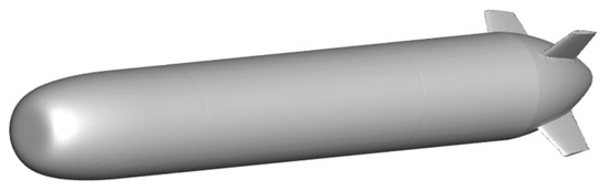
Figure 1.
The AUV model.
2.3. Computational Domain and Boundary Conditions
For the seafloor terrain, this study focuses on dune terrain, which is widely distributed in various environments [18,19,20]. The formation and evolution of these dunes are influenced by hydrodynamic conditions including tides, currents, and waves, sediment levels, water depth, and topography. Scholars have investigated the evolution mechanisms of dunes to varying degrees [21,22,23]. The selection of dune shapes and proportions is based on references such as Omidyeganeh [21] and Van Mierlo [24]. Taking into account the scale of the AUV, the computational domain is established with a total length of 8 L, a height of 1.5 L, and a width of 1.5 L. The establishment of the computational domain and coordinate system is illustrated in Figure 2. The boundary conditions are set with the inlet as a velocity inlet and flow direction along the positive x-axis, and the outlet is set as a pressure outlet. The bottom and the AUV surface are considered a no-slip wall, and the other surfaces are symmetric planes.
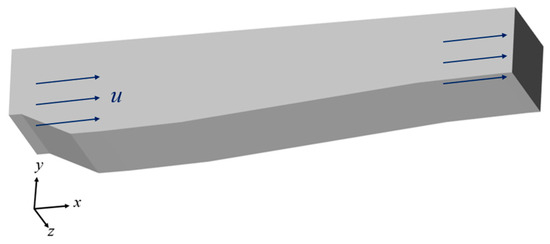
Figure 2.
Computational domain.
Transient simulation is performed in the calculation, and the time step is set between 0.005 s and 0.01 s depending on the flow velocity. The density of water in the computational domain is , and the dynamic viscosity is .
2.4. Dimensionless Hydrodynamic Parameters of the AUV
The dimensionless hydrodynamic parameters relevant to this study include the total resistance coefficient, pressure resistance coefficient, friction resistance coefficient, lift coefficient, pitch moment coefficient, and skin friction coefficient. The distance of the AUV from the seafloor is non-dimensionalized as , where represents the vertical distance from the AUV’s central axis to the seafloor. The resistance coefficient is defined as:
the lift coefficient is defined as:
the pitch moment coefficient is defined as:
and the skin friction coefficient is defined as:
where , , , , and represent the total resistance force, pressure resistance force, friction resistance force, lift force, and pitch moment, respectively, is the incoming flow velocity, is the fluid density, and is the shear stress on the AUV’s surface. The resistance is considered positive along the positive x-axis, the lift is positive along the positive y-axis, and the counterclockwise direction is defined as positive for the pitch moment.
2.5. Grid Generation and Independence Evaluation
In STAR-CCM+, the trimmed cell mesher is used for generating grids, with the focus on refining the grid in the region of turbulent flow around the leeward side of the dune. The wall treatment uses a full method, with the AUV’s surface utilizing a prism layer of five layers and an expansion ratio of 1.1. By setting the thickness of the prism layer, the non-dimensional wall distance is achieved to meet computational requirements. During grid independence evaluation, extreme conditions are considered by placing the AUV very close to the leeward side of the dune. The average resistance acting on the AUV is used as a validation parameter for grid independence evaluation. The results of grid independence evaluation are illustrated in Figure 3. From Figure 3, it can be seen that as the number of grid cells in the computational domain increases, the average resistance acting on the AUV gradually converges. The average resistance values for grid cell numbers of 6.78 million and 9.5 million are already very close. However, performing calculations with a higher number of grid cells would entail significantly higher time costs. Therefore, balancing computational accuracy and efficiency, a grid density corresponding to 6.78 million grid cells is selected for the calculations. In the final simulations, the AUV’s position within the turbulent flow field is considered, with its bow located at a distance of 3.5 m from the inlet. As shown in Figure 4, the number of grids used in the final calculation is about 7 million. The calculations are performed using a 20-core computer, it takes about 48 h to calculate one case.
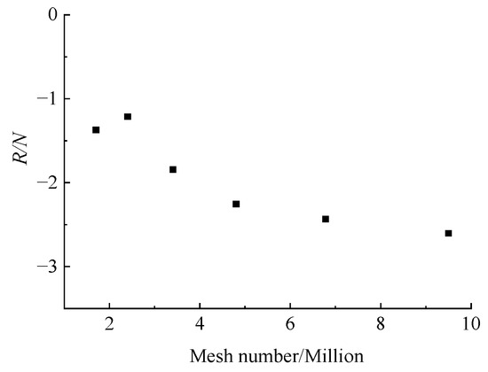
Figure 3.
Grid independence evaluation.
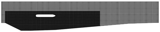
Figure 4.
Grid generation ().
2.6. Numerical Verification Method
The accuracy of the numerical method was verified using the test data of Van Mierlo et al. [24]. Specifically, the experimental data from their T6 test case were selected for comparison. In that experiment, an artificial dune with a length of approximately 1.6 m and a height of about 0.08 m was used. The shape of the dune was the same as that described in Section 2.3 and shown in Figure 5. The flow was in the positive direction of the x-axis. The experiment provided information about the flow field along vertical lines at different downstream distances from the crest of the dune. In this paper, the longitudinal average velocity distributions along vertical lines located at distances of 0.13 m, 0.48 m, 0.82 m, and 1.27 m downstream from the dune crest were selected for verification, as illustrated in Figure 5. Based on the experimental data, a dune model with the same scale as the experiment was established for numerical simulation. To closely match the experimental conditions while ensuring computational efficiency, the length of the calculation domain was set to 1.6 m, the height to 0.37 m, and the width to 1 m. The boundary conditions were set the same way as described in Section 2.3, based on the flow velocity information provided in the experiment at the location closest to the inlet. The test was carried out by changing the flow velocity of the velocity inlet in the simulation and finally setting the flow velocity of the velocity inlet in the simulation to 0.68 m/s to match the experiment.
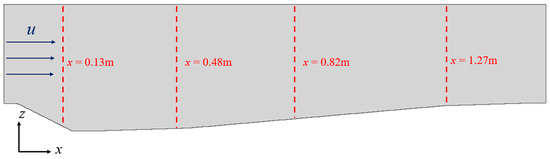
Figure 5.
Diagram showing the vertical line position for recording flow velocity.
Figure 6 shows a comparison between the velocity distributions obtained from numerical simulations and experimental results at different positions along the vertical line. The sampling interval is 150 s, with a sampling frequency of 0.01 s. It can be observed that near the leeward side of the dune, the flow velocity distribution along the vertical line is uneven due to the influence of vortices, and the flow velocity on the vertical line away from the leeward side of the dune tends to be uniform. At the locations where and , there are certain errors between the flow velocity distribution obtained using the numerical simulation and experiment. This may be attributed to the numerical simulation’s inability to account for the actual characteristics of the dune material and the possibility that the boundary conditions were not entirely consistent with real-world conditions. Overall, the results obtained using the numerical method show good agreement with the experimental values, indicating a certain degree of reliability in the numerical approach.
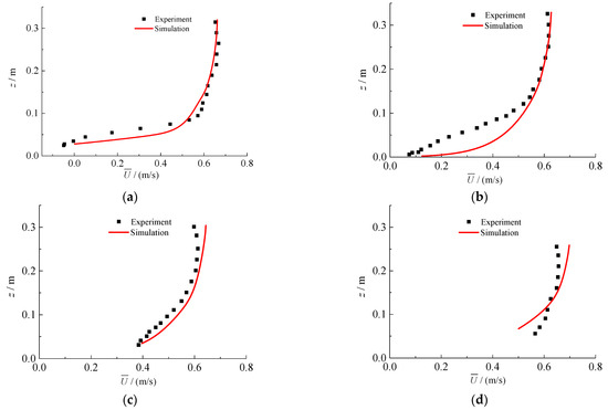
Figure 6.
Comparison between the numerical results and the experimental results: (a) 0.13 m; (b) 0.48 m; (c) 0.82 m; and (d) 1.27 m.
3. Results and Discussion
This study focuses on the instantaneous variation in hydrodynamic coefficients of an AUV within the turbulent flow induced by underwater dune terrain. Considering computational efficiency and the full development of the flow field, the simulation time is set to the duration required for the incoming flow to pass twice the length of the computational domain. The chosen incoming flow velocities are , , and . Notably, due to the more pronounced flow variations at the velocity of , the simulation time is extended to the duration required for the incoming flow to pass four times the length of the computational domain at this velocity. The computational results reveal that, during the initial phase when the incoming flow passes one length of the computational domain at the set velocity, the variation in the AUV’s hydrodynamic coefficients remains relatively stable. In other words, the flow field stays in a relatively stable state without reaching full development. Thus, this study analyzes the variation in the AUV’s hydrodynamic coefficients during the subsequent time intervals beyond this stage.
When , the instantaneous variation in the hydrodynamic coefficients of the AUV at different incoming flow velocities is shown in Figure 7. It can be observed that the hydrodynamic coefficients of the AUV are influenced by the turbulent flow field and fluctuate within a certain range. As the flow velocity increases, the fluctuations become more pronounced. Regarding the total resistance coefficient, which is divided into the shape resistance coefficient and friction resistance coefficient, it becomes apparent that the fluctuation in the shape resistance coefficient is more intense. Moreover, the variation trend in the shape resistance coefficient aligns completely with that of the total resistance coefficient. This suggests that the changes in the AUV’s total resistance are primarily driven by variations in the shape resistance, while the friction resistance coefficient shows relatively minor fluctuations and remains nearly stable under different flow velocities. The shape resistance and friction resistance are determined by integrating pressure and shear forces over the AUV’s surface. At a flow velocity of , the pressure distribution on the upper and lower sides of the AUV’s longitudinal section in a center plane at different instances is shown in Figure 8. It is evident that due to the presence of the seafloor, the pressure variations in the lower surface of the AUV, especially in the bow and stern sections, are more pronounced. Figure 9 presents the distribution of the skin friction coefficient on the AUV’s surface at different instances. Similarly, significant variations in shear forces can be observed in the bow and stern sections of the AUV, with minor fluctuations in the midsection. Overall, among the various hydrodynamic coefficients, the lift coefficient presents the most pronounced fluctuations.
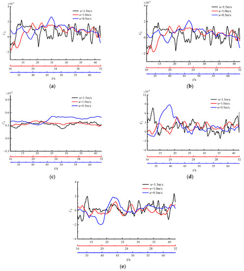
Figure 7.
Instantaneous variation in the hydrodynamic coefficients of the AUV at different incoming flow velocities; : (a) total resistance coefficient; (b) pressure resistance coefficient; (c) friction resistance coefficient; (d) lift coefficient; and (e) pitch moment coefficient.
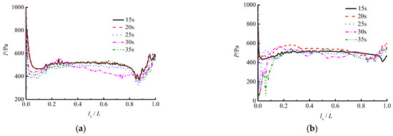
Figure 8.
Pressure distribution on the upper and lower sides of the AUV’s longitudinal section in the center plane at different times; and : (a) upper side and (b) lower side.
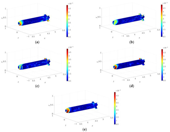
Figure 9.
Skin friction coefficient distribution on the AUV’s surface at different times; and : (a) 15 s; (b) 20 s; (c) 25 s; (d) 30 s; and (e) 35 s.
When , the variation in the hydrodynamic coefficients of the AUV at different distances from the seafloor is shown in Figure 10. It can be observed that the coefficients are influenced by the underwater dune terrain, and the influence on the AUV diminishes as the distance between the AUV and the seafloor increases. When , the fluctuations in the AUV’s hydrodynamic coefficients become negligible. However, concerning the friction resistance coefficient, significant fluctuations only occur when the AUV is positioned relatively close to the seafloor. This indicates that the instantaneous influence of turbulence variations on the AUV’s friction resistance is minimal.
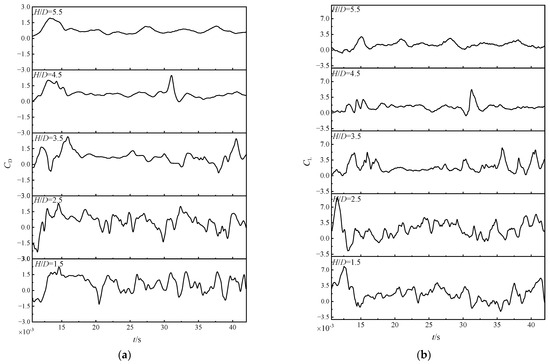
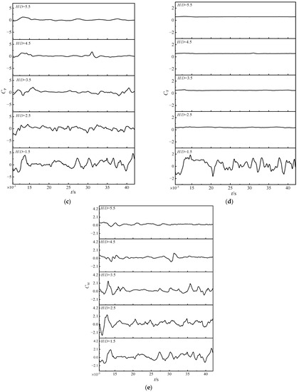
Figure 10.
Instantaneous variation in the hydrodynamic coefficients of the AUV at different distances from the seafloor; : (a) total resistance coefficient; (b) pressure resistance coefficient; (c) friction resistance coefficient; (d) lift coefficient; and (e) pitch moment coefficient.
To analyze the characteristics of hydrodynamic coefficient variations in turbulent flow fields, a Fourier analysis is performed on the time-domain variation curves of the AUV’s hydrodynamic coefficients for different incoming flow velocities. This analysis yields the amplitude–frequency variation curves of the hydrodynamic coefficients. The peaks are selected from these curves, and within a 2% bandwidth on either side of the peak frequency in the amplitude-frequency curve, a bandpass filter is applied to the original curves. This process results in the time-domain variation curves of hydrodynamic coefficients corresponding to the peak frequency.
When , the Fourier analysis and filtering results of the time-domain hydrodynamic coefficient curves for different incoming flow velocities are shown in Appendix A, Figure A1, Figure A2, Figure A3, Figure A4, Figure A5, Figure A6, Figure A7, Figure A8 and Figure A9. It can be observed that higher amplitude is associated with high-frequency components when the flow velocity is relatively high. As shown in Figure 11 and Figure 12, within the turbulent region on the leeward side of the dune, a continuous process of vortex evolution and fragmentation occurs. When the flow velocity is high, the flow field possesses increased energy, leading to more intense vortex motion and promoting the fragmentation of smaller vortices. The dominance of high-frequency components in the flow field, along with the increased amplitudes of high-frequency phenomena, indicates the accelerated development of small vortices, enhancing the randomness of the flow field and resulting in pronounced variations in the AUV’s hydrodynamic coefficients. As the flow velocity decreases, the dominant components in the curves shift toward lower frequencies, accompanied by a reduction in the amplitude of high-frequency components. This shift implies a weakening in the phenomenon of vortex evolution and fragmentation, with large-scale vortices constituting the main components of the flow field while evolving at a slower pace. Furthermore, it is evident that with decreasing flow velocity, the dominance of low-frequency components is most pronounced in the resistance coefficient’s time-domain curve. However, for the lift coefficient and pitch moment coefficient time-domain curves, the frequency components dominating the behavior at low flow velocities are higher than those in the resistance coefficient curve. This indicates that the AUV’s lift and pitch moment present higher sensitivity to variations in the turbulent flow field, with the potential for significant changes still present at lower flow velocities.
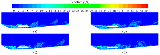
Figure 11.
Vorticity distribution contours at different times; and : (a) 30 s; (b) 31 s; (c) 32 s; and (d) 33 s.
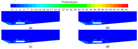
Figure 12.
Vorticity distribution contours at different times; and : (a) 40 s; (b) 41 s; (c) 42 s; and (d) 43 s.
When , the Fourier analysis and filtering results of the time-domain hydrodynamic coefficient curves for different near-seafloor distances are presented in Appendix A, Figure A10, Figure A11, Figure A12, Figure A13, Figure A14, Figure A15, Figure A16, Figure A17, Figure A18, Figure A19, Figure A20 and Figure A21. Within the range of H/D = 1.5 to 3.5, the hydrodynamic coefficient time-domain curves present larger amplitudes of high-frequency components. The vorticity distribution contours at different near-seafloor distances in the final time step are shown in Figure 13. Due to the shear layer generated by the seafloor terrain, the flow field within this region is more turbulent. Moving away from this region, the intensity of vortex motion decreases, leading to a reduction in the frequency of flow field variations, and the dominance of low-frequency components in the hydrodynamic coefficient time-domain curves becomes evident. Furthermore, it is noteworthy that the dominant frequency component in the pitch moment coefficient time-domain curves is higher than the other two coefficients. This indicates that the AUV is prone to experiencing pitching motion in this turbulent flow field. As the AUV moves away from this region, the frequency and intensity of pitching motion will significantly decrease. However, during near-seafloor processes, the intense pitching motion could potentially pose collision risks.
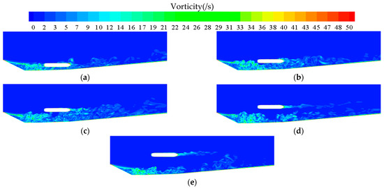
Figure 13.
Vorticity distribution contours at different near-seafloor distances at the final time step; : (a) ; (b) ; (c) ; (d) ; and (e) .
Along the length of the AUV, the turbulent kinetic energy k is calculated at 0.05 m from the upper and lower surfaces of the AUV in the longitudinal section of the AUV in the center plane. The distribution of turbulent kinetic energy near the AUV is shown in Figure 14 and Figure 15, where is the longitudinal distance between the AUV surface and the AUV bow. It is evident that as the distance from the seafloor decreases, the turbulent kinetic energy near the AUV increases, which indicates that the fluid possesses greater energy and is more prone to forming vortex structures. Interestingly, it can be observed that when H/D = 2.5, the turbulent kinetic energy beneath the AUV is higher than when H/D = 1.5. However, such a phenomenon is not observed in the variation in turbulent kinetic energy above the AUV. Analyzing Figure 13 reveals that this is because, at smaller near-seafloor distances, the presence of the AUV hampers the development of vortex structures between the AUV and the seafloor. To depict the vortex characteristics within the flow field more distinctly, the Q-criterion method is used for identification. Figure 16 displays the vortex structures corresponding to Q = 10 in the flow field. For H/D = 1.5, the presence of the AUV limits the development of vortex structures beneath it, reducing their quantity. However, the AUV remains within the vortex structures, leading to continually changing forces exerted on the AUV. Moreover, the presence of the AUV affects the evolution of vortex structures. Notably, it can be observed that at smaller near-seafloor distances, the turbulent kinetic energy around the lower surface of the AUV gradually diminishes along the AUV’s longitudinal direction. This phenomenon arises because the bow of the AUV is located within a region with stronger vortex structures, which may result in vibration in practical applications.
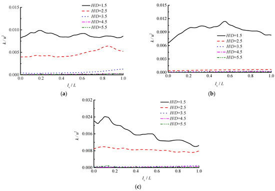
Figure 14.
Dimensionless turbulent kinetic energy at 0.05 m from the upper surface of the AUV in the longitudinal section of the AUV in center plane: (a) ; (b) ; and (c) .
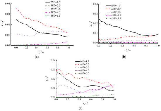
Figure 15.
Dimensionless turbulent kinetic energy at 0.05 m from the lower surface of the AUV in the longitudinal section of the AUV in center plane: (a) ; (b) ; and (c) .
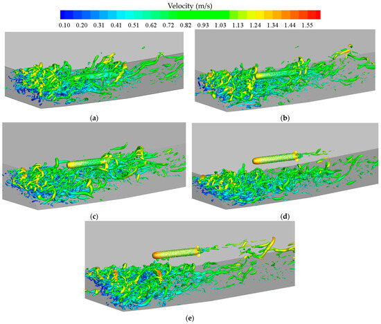
Figure 16.
Vortex structure distribution at the final time step (); : (a) ; (b) ; (c) ; (d) ; and (e) .
Below is an analysis of the average characteristics of the AUV hydrodynamic changes. The average values of the AUV hydrodynamic coefficients under different incoming flow velocities and near-seafloor distances are listed in Table 1. Higher flow velocities correspond to a reduction in the resistance coefficient value. As near-seafloor distance varies, there is no distinct pattern in the variation in the hydrodynamic coefficients. Overall, the total resistance coefficient presents an increasing trend with the increase in near-seafloor distance. This increase in the total resistance coefficient is primarily driven by the rise in the friction resistance coefficient.

Table 1.
Average values of the AUV hydrodynamic coefficients.
Figure 17 shows the distribution of the average skin friction coefficients of the AUV for at different near-seafloor distances. It is evident that with increasing near-seafloor distance, the average skin friction coefficient on the AUV surface gradually increases. Figure 18 presents velocity distribution contours around the AUV. Influenced by the terrain, the leeward side of the dune presents lower flow velocities. As it moves farther away from the seafloor, the flow velocities increase, and consequently, the shear stress on the AUV surface increases, leading to an increase in friction resistance. However, it is observable that the average skin friction coefficient in the stern region of the AUV decreases with increasing near-seafloor distance. Figure 19 shows the vortex structures in the flow field near the AUV at the final moment for and , with Q = 30. In regions with higher flow velocities far from the seafloor, the shedding of stern vortices of the AUV becomes more obvious, leading to easier flow separation in the region near the stern, which results in a reduction in shear stress on the stern surface.
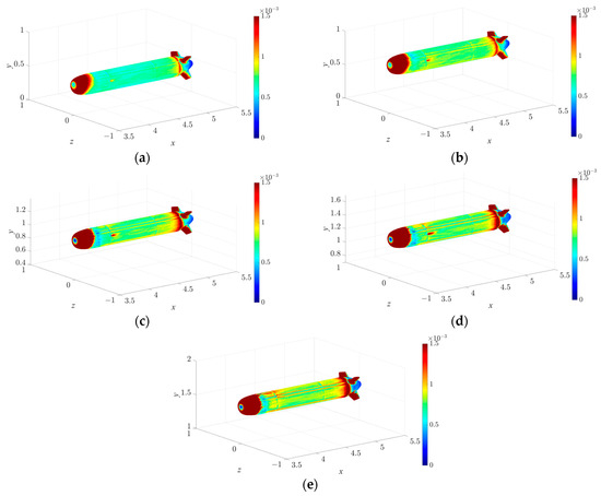
Figure 17.
Average skin friction coefficient distribution of the AUV at different near-seafloor distances; : (a) ; (b) ; (c) ; (d) ; and (e) .
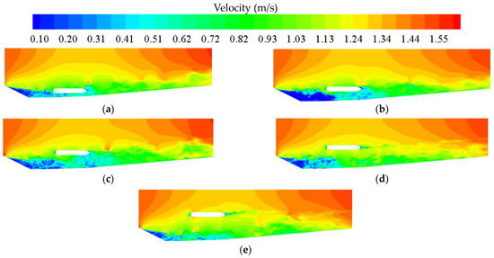
Figure 18.
Velocity distribution contours around the AUV at different near-seafloor distances; : (a) ; (b) ; (c) ; (d) ; and (e) .
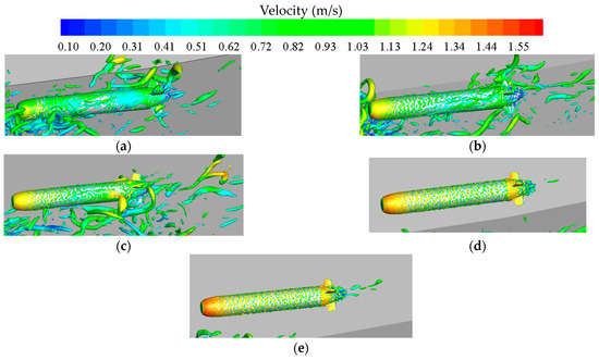
Figure 19.
Vortex structure distribution near the AUV in the final time step (); : (a) ; (b) ; (c) ; (d) ; and (e) .
Regarding the lift coefficient, there is a general trend indicating a decreasing lift coefficient as the near-seafloor distance increases. Figure 20 displays pressure distribution contours around the AUV. It is evident that as the near-seafloor distance increases, the pressure beneath the AUV decreases, leading to reduced pressure differences between the upper and lower surfaces and subsequently lowering the lift coefficient.
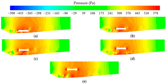
Figure 20.
Pressure distribution contours around the AUV at different near-seafloor distances; : (a) ; (b) ; (c) ; (d) ; and (e) .
Figure 21 and Figure 22 present comparisons among the average pressure distribution on the upper and lower sides in the longitudinal section of the AUV in the center plane at different incoming flow velocities for and at different near-seafloor distances for , respectively. It is evident that higher flow velocities correspond to greater average pressures on the AUV surface. The average pressure fluctuations are more pronounced in the bow and stern regions. Moreover, as the near-seafloor distance increases, the average surface pressure on the AUV decreases.
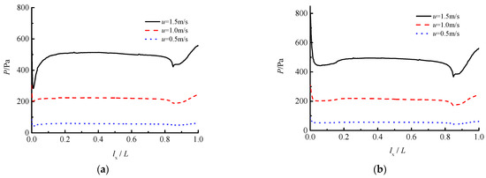
Figure 21.
Average pressure distribution on the upper and lower sides in the longitudinal section of the AUV in the center plane at different near-seafloor distances; : (a) upper side and (b) lower side.
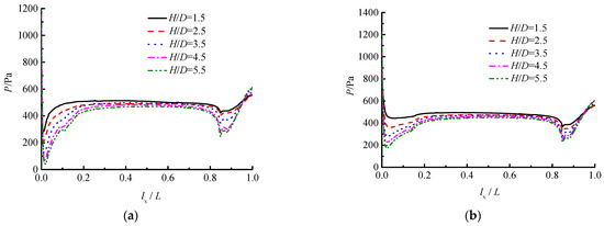
Figure 22.
Average pressure distribution on the upper and lower sides in the longitudinal section of the AUV in the center plane at different incoming flow velocities; : (a) upper side and (b) lower side.
Figure 23 illustrates a comparison between the average pressures on the upper and lower sides in the longitudinal section of the AUV in the center plane for different near-seafloor distances when . It is observable that as the near-seafloor distance increases, the average pressures near the bow and stern of the AUV become more similar.
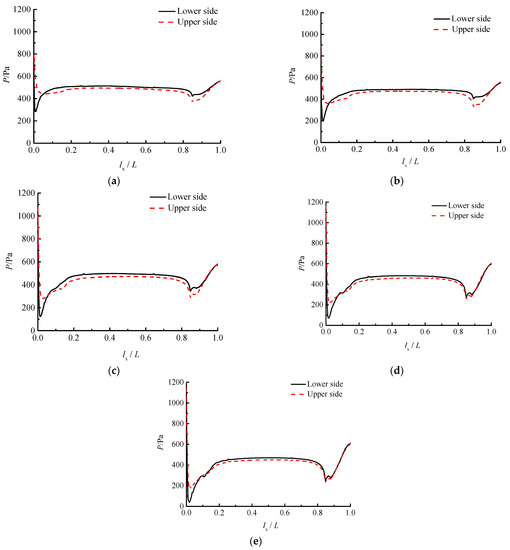
Figure 23.
Comparison between the average pressures on the upper and lower sides in the longitudinal section of the AUV in the center plane at different near-seafloor distances; : (a) ; (b) ; (c) ; (d) ; and (e) .
4. Conclusions
AUVs play an increasingly significant role in marine exploration. However, existing assessments of AUV maneuverability and navigation design often neglect unsteady hydrodynamic disturbances caused by the seafloor. In this study, an analysis of the hydrodynamic performance of AUVs in turbulent flow fields generated by underwater dunes was conducted. The AUV was placed about 3 m from the crest of the dune. Using the LES method, the hydrodynamic characteristics of the AUV and flow field variations were investigated under different flow velocities and near-seafloor distances. The results of this study include the following. In turbulent flow fields, the hydrodynamic coefficients of the AUV present fluctuations within a certain range, which become more pronounced with increasing flow velocity. In the range studied in this paper, the amplitude of the curve fluctuation in the hydrodynamic coefficient can reach about 2–8 times its mean value. Among these coefficients, the variation in the pressure resistance coefficient predominantly affects the total resistance coefficient. The friction resistance coefficient of the AUV presents relatively minor fluctuations under different flow velocities and is less affected by turbulent flow fields. The lift coefficient and pitch moment coefficient are more sensitive to variations in the turbulent flow field, with higher flow velocities resulting in more pronounced changes. As the distance between the AUV and the seafloor increases, the fluctuations in the hydrodynamic coefficients gradually diminish, particularly for the resistance coefficient. Overall, when , the AUV moves away from the region of the flow field where turbulence is significant, and the influence of turbulence on the hydrodynamic performance of the AUV becomes negligible. Regarding the frictional drag, it remains relatively stable when . Additionally, when , the AUV hampers the formation of vortices below it.
In summary, the hydrodynamic performance of AUVs in turbulent flow fields caused by the underwater dune is influenced by the constantly changing flow field structure. This effect is particularly pronounced in high flow velocity conditions and when the AUV is situated closer to the seafloor. While this study provides an exploration of the hydrodynamic performance of AUVs in underwater dune terrain, further experimental validation and engineering applications are required. Future research can combine real-world scenarios to optimize AUV design and control strategies, adapting them to complex seafloor environments.
Author Contributions
Conceptualization, Y.G. and P.L.; methodology, Y.G. and P.L.; validation, Y.G.; formal analysis, Y.G. and P.L.; investigation, Y.G. and P.L.; resources, H.Q.; data curation, Y.G.; writing—original draft preparation, Y.G.; writing—review and editing, Y.G. and P.L.; visualization, Y.G., Z.L. and J.G.; funding acquisition, P.L. All authors have read and agreed to the published version of the manuscript.
Funding
This work was funded by the National Natural Science Foundation of China, grant number 52231011), the Research Fund from Stable Supporting Fund of Science and Technology on Underwater Vehicle Technology, grant number JCKYS2022SXJQR-11, and the “Chunhui Project” Cooperative Scientific Research Foundation of Ministry of Education of China, grant number 202200288.
Institutional Review Board Statement
Not applicable.
Informed Consent Statement
Not applicable.
Data Availability Statement
Data available in a publicly accessible repository.
Conflicts of Interest
The authors declare no conflict of interest.
Appendix A
When , a Fourier analysis was performed on the time-domain curves of the AUV’s total drag coefficient, lift coefficient, and pitch moment coefficient under different inflow velocities. Based on the results of the Fourier analysis, the original time-domain curves were filtered to obtain the time-domain curves of the hydrodynamic coefficients corresponding to the main frequency components.

Figure A1.
Fourier analysis and filtering results of the time-domain total resistance coefficient curves; and : (a) amplitude–frequency variation curve; (b) filtered time-domain curve corresponding to 0.256 Hz; (c) filtered time-domain curve corresponding to 0.447 Hz; and (d) filtered time-domain curve corresponding to 0.619 Hz.


Figure A2.
Fourier analysis and filtering results of the time-domain total resistance coefficient curves; and : (a) amplitude–frequency variation curve; (b) filtered time-domain curve corresponding to 0.062 Hz; and (c) filtered time-domain curve corresponding to 0.562 Hz.
Figure A2.
Fourier analysis and filtering results of the time-domain total resistance coefficient curves; and : (a) amplitude–frequency variation curve; (b) filtered time-domain curve corresponding to 0.062 Hz; and (c) filtered time-domain curve corresponding to 0.562 Hz.


Figure A3.
Fourier analysis and filtering results of the time-domain total resistance coefficient curves; and : (a) amplitude–frequency variation curve; (b) filtered time-domain curve corresponding to 0.187 Hz; and (c) filtered time-domain curve corresponding to 0.032 Hz.
Figure A3.
Fourier analysis and filtering results of the time-domain total resistance coefficient curves; and : (a) amplitude–frequency variation curve; (b) filtered time-domain curve corresponding to 0.187 Hz; and (c) filtered time-domain curve corresponding to 0.032 Hz.


Figure A4.
Fourier analysis and filtering results of the time-domain total resistance coefficient curves; and : (a) amplitude–frequency variation curve; (b) filtered time-domain curve corresponding to 0.064 Hz; and (c) filtered time-domain curve corresponding to 0.287 Hz.
Figure A4.
Fourier analysis and filtering results of the time-domain total resistance coefficient curves; and : (a) amplitude–frequency variation curve; (b) filtered time-domain curve corresponding to 0.064 Hz; and (c) filtered time-domain curve corresponding to 0.287 Hz.


Figure A5.
Fourier analysis and filtering results of the time-domain total resistance coefficient curves; and : (a) amplitude–frequency variation curve; (b) filtered time-domain curve corresponding to 0.250 Hz; and (c) filtered time-domain curve corresponding to 0.562 Hz.
Figure A5.
Fourier analysis and filtering results of the time-domain total resistance coefficient curves; and : (a) amplitude–frequency variation curve; (b) filtered time-domain curve corresponding to 0.250 Hz; and (c) filtered time-domain curve corresponding to 0.562 Hz.


Figure A6.
Fourier analysis and filtering results of the time-domain total resistance coefficient curves; and : (a) amplitude–frequency variation curve and (b) filtered time-domain curve corresponding to 0.062 Hz.
Figure A6.
Fourier analysis and filtering results of the time-domain total resistance coefficient curves; and : (a) amplitude–frequency variation curve and (b) filtered time-domain curve corresponding to 0.062 Hz.


Figure A7.
Fourier analysis and filtering results of the time-domain total resistance coefficient curves; and : (a) amplitude–frequency variation curve; (b) filtered time-domain curve corresponding to 0.287 Hz; and (c) filtered time-domain curve corresponding to 0.351 Hz.
Figure A7.
Fourier analysis and filtering results of the time-domain total resistance coefficient curves; and : (a) amplitude–frequency variation curve; (b) filtered time-domain curve corresponding to 0.287 Hz; and (c) filtered time-domain curve corresponding to 0.351 Hz.


Figure A8.
Fourier analysis and filtering results of the time-domain total resistance coefficient curves; and : (a) amplitude–frequency variation curve; (b) filtered time-domain curve corresponding to 0.187 Hz; and (c) filtered time-domain curve corresponding to 0.312 Hz.
Figure A8.
Fourier analysis and filtering results of the time-domain total resistance coefficient curves; and : (a) amplitude–frequency variation curve; (b) filtered time-domain curve corresponding to 0.187 Hz; and (c) filtered time-domain curve corresponding to 0.312 Hz.


Figure A9.
Fourier analysis and filtering results of the time-domain total resistance coefficient curves; and : (a) amplitude–frequency variation curve and (b) filtered time-domain curve corresponding to 0.094 Hz.
Figure A9.
Fourier analysis and filtering results of the time-domain total resistance coefficient curves; and : (a) amplitude–frequency variation curve and (b) filtered time-domain curve corresponding to 0.094 Hz.

When , a Fourier analysis was performed on the time-domain curves of the AUV’s total drag coefficient, lift coefficient, and pitch moment coefficient under different near-seafloor distances. Based on the results of the Fourier analysis, the original time-domain curves were filtered to obtain the time-domain curves of the hydrodynamic coefficients corresponding to the main frequency components.

Figure A10.
Fourier analysis and filtering results of the time-domain total resistance coefficient curves; and : (a) amplitude–frequency variation curves and (b) filtered time-domain curve corresponding to 0.224 Hz.
Figure A10.
Fourier analysis and filtering results of the time-domain total resistance coefficient curves; and : (a) amplitude–frequency variation curves and (b) filtered time-domain curve corresponding to 0.224 Hz.


Figure A11.
Fourier analysis and filtering results of the time-domain total resistance coefficient curves; and : (a) amplitude–frequency variation curv; (b) filtered time-domain curve corresponding to 0.287 Hz; and (c) filtered time-domain curve corresponding to 0.160 Hz; (d) Filtered time-domain curve corresponding to 0.607 Hz.


Figure A12.
Fourier analysis and filtering results of the time-domain total resistance coefficient curves; and : (a) amplitude–frequency variation curve; (b) filtered time-domain curve corresponding to 0.064 Hz; (c) filtered time-domain curve corresponding to 0.224 Hz; (d) filtered time-domain curve corresponding to 0.128 Hz; and (e) filtered time-domain curve corresponding to 0.287 Hz.


Figure A13.
Fourier analysis and filtering results of the time-domain total resistance coefficient curves; and : (a) amplitude–frequency variation curve; (b) filtered time-domain curve corresponding to 0.160 Hz; and (c) filtered time-domain curve corresponding to 0.287 Hz.
Figure A13.
Fourier analysis and filtering results of the time-domain total resistance coefficient curves; and : (a) amplitude–frequency variation curve; (b) filtered time-domain curve corresponding to 0.160 Hz; and (c) filtered time-domain curve corresponding to 0.287 Hz.


Figure A14.
Fourier analysis and filtering results of the time-domain total resistance coefficient curves; and : (a) amplitude–frequency variation curve; (b) filtered time-domain curve corresponding to 0.064 Hz; (c) filtered time-domain curve corresponding to 0.447 Hz; and (d) filtered time-domain curve corresponding to 0.256 Hz.


Figure A15.
Fourier analysis and filtering results of the time-domain total resistance coefficient curves; and : (a) amplitude–frequency variation curve; (b) filtered time-domain curve corresponding to 0.192 Hz; and (c) filtered time-domain curve corresponding to 0.415 Hz.
Figure A15.
Fourier analysis and filtering results of the time-domain total resistance coefficient curves; and : (a) amplitude–frequency variation curve; (b) filtered time-domain curve corresponding to 0.192 Hz; and (c) filtered time-domain curve corresponding to 0.415 Hz.


Figure A16.
Fourier analysis and filtering results of the time-domain total resistance coefficient curves; and : (a) amplitude–frequency variation curve; (b) filtered time-domain curve corresponding to 0.224 Hz; (c) filtered time-domain curve corresponding to 0.383 Hz; (d) filtered time-domain curve corresponding to 0.064 Hz; (e) filtered time-domain curve corresponding to 0.128 Hz; and (f) filtered time-domain curve corresponding to 0.767 Hz.


Figure A17.
Fourier analysis and filtering results of the time-domain total resistance coefficient curves; and : (a) amplitude–frequency variation curve; (b) filtered time-domain curve corresponding to 0.224 Hz; (c) filtered time-domain curve corresponding to 0.160 Hz; and (d) filtered time-domain curve corresponding to 0.160 Hz.


Figure A18.
Fourier analysis and filtering results of the time-domain total resistance coefficient curves; and : (a) amplitude–frequency variation curve; (b) filtered time-domain curve corresponding to 0.287 Hz; (c) filtered time-domain curve corresponding to 0.383 Hz; and (d) filtered time-domain curve corresponding to 0.128 Hz.


Figure A19.
Fourier analysis and filtering results of the time-domain total resistance coefficient curves; and : (a) amplitude–frequency variation curve; (b) filtered time-domain curve corresponding to 0.351 Hz; (c) filtered time-domain curve corresponding to 0.224 Hz; (d) filtered time-domain curve corresponding to 0.415 Hz; (e) filtered time-domain curve corresponding to 0.160 Hz; and (f) filtered time-domain curve corresponding to 0.160 Hz.


Figure A20.
Fourier analysis and filtering results of the time-domain total resistance coefficient curves; , and : (a) amplitude–frequency variation curve; (b) filtered time-domain curve corresponding to 0.256 Hz; and (c) filtered time-domain curve corresponding to 0.383 Hz.
Figure A20.
Fourier analysis and filtering results of the time-domain total resistance coefficient curves; , and : (a) amplitude–frequency variation curve; (b) filtered time-domain curve corresponding to 0.256 Hz; and (c) filtered time-domain curve corresponding to 0.383 Hz.


Figure A21.
Fourier analysis and filtering results of the time-domain total resistance coefficient curves; and : (a) amplitude–frequency variation curve; (b) filtered time-domain curve corresponding to 0.096 Hz; (c) filtered time-domain curve corresponding to 0.287 Hz; (d) filtered time-domain curve corresponding to 0.224 Hz; (e) filtered time-domain curve corresponding to 0.479 Hz; and (f) filtered time-domain curve corresponding to 0.160 Hz.


References
- Sahoo, A.; Dwivedy, S.K.; Robi, P.S. Advancements in the field of autonomous underwater vehicle. Ocean. Eng. 2019, 181, 145–160. [Google Scholar] [CrossRef]
- Wakita, N.; Hirokawa, K.; Ichikawa, T.; Yamauchi, Y. Development of autonomous underwater vehicle (AUV) for exploring deep sea marine mineral resources. Mitsubishi Heavy Ind. Tech. Rev. 2010, 47, 73–80. [Google Scholar]
- Korol, Y.M.; Valeri, N.; Brazhko, A.; Ursolov, A.; Moonesun, M. Bottom effect on the submarine moving close to the sea bottom. J. Sci. Eng. Res. 2016, 6, 106–113. [Google Scholar]
- Heng, L.L. Design and Application of Underwater Visual Ranging System. Master’s Thesis, Hangzhou Dianzi University, Hangzhou, China, 2014. [Google Scholar]
- Kim, K.; Ura, T. Terrain-adaptive optimal guidance for near-bottom survey by an autonomous underwater vehicle. In Proceedings of the 2013 IEEE International Underwater Technology Symposium (UT), Tokyo, Japan, 5–8 March 2013. [Google Scholar]
- Kuang, X.F.; Miao, Q.M.; Cheng, D.M. Study on hydrodynamic numerical calculation of submarine sailing near seabed. In Proceedings of the Ship Hydrodynamics Conference, St. Johns, NL, Canada, 25–26 September 2004. [Google Scholar]
- Wu, B.S.; Xing, F.; Kuang, X.F.; Miao, Q.M. Investigation of hydrodynamic characteristics of submarine moving close to the sea bottom with CFD methods. J. Ship Mech. 2005, 9, 19–28. [Google Scholar]
- Du, X.X.; Wang, H.; Hao, C.Z.; Li, X.L. Analysis of hydrodynamic characteristics of unmanned underwater vehicle moving close to the sea bottom. Def. Technol. 2014, 10, 76–81. [Google Scholar] [CrossRef]
- Zhu, A.J.; Ying, L.M.; Zheng, H.; Shen, H.C. Resistance test method on underwater vessel operating close to the bottom or the surface. J. Ship Mech. 2012, 16, 368–374. [Google Scholar]
- Chen, C.W.; Yan, N.M. Prediction of added mass for an autonomous underwater vehicle moving near sea bottom using panel method. In Proceedings of the 2017 4th International Conference on Information Science and Control Engineering (ICISCE), Changsha, China, 21–23 July 2017. [Google Scholar]
- Wu, L.; Li, S.; Feng, X.; Jiang, H.; Zhang, X.; Hu, W. Unsteady simulation of AUVs approaching seafloor by self-propulsion using multi-block hybrid dynamic grid method. J. Fluids Struct. 2022, 114, 103728. [Google Scholar] [CrossRef]
- Liu, T.S. Submarine Topography and Pipeline for AUV Hydrodynamic Performance Interference Analysis. Master’s Thesis, Harbin Engineering University, Harbin, China, 2015. [Google Scholar]
- Yan, T.H.; Ma, D.F.; Xue, X.F.; Chen, X.K. Analysis of Hydrodynamic Characteristics of Autonomous Underwater Vehicle Close to Sea Bottom. Comput. Simul. 2016, 33, 301–305 + 327. [Google Scholar]
- Mitra, A.; Panda, J.P.; Warrior, H.V. Experimental and numerical investigation of the hydrodynamic characteristics of autonomous underwater vehicles over sea-beds with complex topography. Ocean. Eng. 2020, 198, 106978. [Google Scholar] [CrossRef]
- Guo, J.; Lin, Y.; Lin, P.; Li, H.; Huang, H.; Chen, Y. Study on hydrodynamic characteristics of the disk-shaped autonomous underwater helicopter over sea-beds. Ocean. Eng. 2022, 266, 113132. [Google Scholar] [CrossRef]
- Mitra, A.; Panda, J.P.; Warrior, H.V. The effects of free stream turbulence on the hydrodynamic characteristics of an AUV hull form. Ocean. Eng. 2019, 174, 148–158. [Google Scholar] [CrossRef]
- Mitra, A.; Panda, J.P.; Warrior, H.V. The hydrodynamic characteristics of Autonomous Underwater Vehicles in rotating flow fields. Proc. Inst. Mech. Eng. Part M J. Eng. Marit. Environ. 2021. [Google Scholar] [CrossRef]
- Wynn, R.B.; Masson, D.G.; Stow, D.A.; Weaver, P.P. Turbidity current sediment waves on the submarine slopes of the western Canary Islands. Mar. Geol. 2000, 163, 185–198. [Google Scholar] [CrossRef]
- Wynn, R.B.; Stow, D.A. Classification and characterisation of deep-water sediment waves. Mar. Geol. 2002, 192, 7–22. [Google Scholar] [CrossRef]
- Reeder, D.B.; Ma, B.B.; Yang, Y.J. Very large subaqueous sand dunes on the upper continental slope in the South China Sea generated by episodic, shoaling deep-water internal solitary waves. Mar. Geol. 2011, 279, 12–18. [Google Scholar] [CrossRef]
- Omidyeganeh, M.; Piomelli, U. Large-eddy simulation of three-dimensional dunes in a steady, unidirectional flow. Part 1. Turbulence statistics. J. Fluid Mech. 2013, 721, 454–483. [Google Scholar] [CrossRef]
- Omidyeganeh, M.; Piomelli, U. Large-eddy simulation of three-dimensional dunes in a steady, unidirectional flow. Part 2. Flow structures. J. Fluid Mech. 2013, 734, 509–534. [Google Scholar] [CrossRef][Green Version]
- Venditti, J.G.; Bauer, B.O. Turbulent flow over a dune: Green River, Colorado. Earth Surf. Process. Landf. J. Br. Geomorphol. Res. Group 2005, 30, 289–304. [Google Scholar] [CrossRef]
- Van Mierlo, M.C.L.M.; De Ruiter, J.C.C. Turbulence Measurements above Artificial Dunes; Delft Hydraulics Lab: Delft, The Netherlands, 1988. [Google Scholar]


Disclaimer/Publisher’s Note: The statements, opinions and data contained in all publications are solely those of the individual author(s) and contributor(s) and not of MDPI and/or the editor(s). MDPI and/or the editor(s) disclaim responsibility for any injury to people or property resulting from any ideas, methods, instructions or products referred to in the content. |
© 2023 by the authors. Licensee MDPI, Basel, Switzerland. This article is an open access article distributed under the terms and conditions of the Creative Commons Attribution (CC BY) license (https://creativecommons.org/licenses/by/4.0/).