Abstract
The aerodynamics of high-speed vehicles in evacuated tunnels is studied with particular reference to the consequences of choked flow conditions at the tails of the vehicles. It is shown that this has a dominant influence on overall conditions (pressure, temperature, velocity). Together with the need for the evacuated tunnel system to be closed, the high speeds cause the aerodynamic behaviour to differ greatly from that in conventional railway tunnels. A key purpose of the paper is to assess the relative importance of a large range of parameters and, for clarity, this is completed by focussing on a single vehicle in a single tunnel that is closed at both ends. Consideration is then given to interactions between more than one vehicle and to a twin-tube tunnel configuration in which interactions occur between vehicles moving in opposite directions. The paper closes with a brief mention of system-dependent matters that need to be considered in addition to the generic parameters investigated herein.
1. Introduction
The aerodynamics of trains in tunnels have been studied extensively during the past century, with the result that most of the phenomena that need to be considered by designers are well understood. Whilst it remains the case that some cannot be predicted with high confidence (e.g., wavefront steepening in long tunnels and its consequences for the emission of micro-pressure waves), all important ones are well understood in principle (e.g., Niu et al. 2020 [1]). The same cannot safely be said for vehicles travelling at high speeds in tunnels that have been evacuated to very low pressures, notwithstanding the existence of studies providing valuable guidance (e.g., Kauzinyte et al. 2019 [2]). No operational systems of this type currently exist, although extensive effort continues to be devoted to assessing many aspects of them—e.g., Bizzozero, et al. (2021) [3], Museros, et al. (2021) [4], Nick and Sato (2020) [5], Tudor and Paolone (2021) [6]. Also, whereas various authors have addressed the aerodynamic behaviour in detail, most focus on flows local to the vehicle itself, usually with the primary purpose of reducing “form” drag—e.g., Braun et al. (2017) [7], Chen et al. (2012) [8], Opgenoord and Caplan (2018) [9] and Zhang (2012) [10]. It is therefore considered that a generic assessment of the relevant aerodynamics could be of value, and this paper is intended as a contribution to that process.
The author’s first involvement in the design of this type of railway was in connection with the Swissmetro project in the 1990s (Swissmetro 1999 [11]). Early plans for this related solely to Switzerland, although the designers subsequently had ambitions for major extensions of the scheme through much of Europe—as is also envisaged today. Initially, the intention was to operate the tunnels at very low pressure, primarily to reduce aerodynamic drag—and hence also the required power. However, the target ambient pressure increased as the project developed and pressures in the order of 10 kPa (i.e., 10% of an atmosphere) became seen as preferable. This was the result of many factors, not all of which related to airflows generated by the vehicles. Herein, however, only the latter are considered. This is because the paper is not intended to be indicative of any particular system or even any particular conceptual design. Instead, its purpose is to provide background information for persons responsible for studying such systems.
Differences from studies of high-speed trains in conventional railways can be illustrated by asking questions such as:
- Will high vehicle speeds cause sonic airspeeds and hence choked flow conditions?
- Will the low ambient pressures ensure relatively low maximum pressures?
- Will the low ambient pressures ensure relatively low maximum temperatures?
- Will the low ambient pressures have a strong influence on heat flows?
- How will multiple vehicles interact aerodynamically?
- How beneficial will it be to link tunnels with vehicles travelling in opposite directions?
Readers who are able to answer such questions with high confidence need not read further. Others should expect to find some useful pointers although it is re-emphasised that the aim is to provide generic guidance, not to suggest the relative importance of the various phenomena in specific design studies.
1.1. Theoretical Methodology
All simulations presented herein are based on one-dimensional (1-D) analysis, using the software package ThermoTun (2022) [12]. This is readily available to the author, but any other software with appropriate capabilities could be equally suitable for a generic study such as this. The theoretical basis of the software is outlined in Appendix A. It is not claimed that any aspect of it should be regarded as novel. Rather, it is based on equations that have been known since the 19th century (or earlier). However, the extension of the code to flow Mach numbers up to one is relatively recent (Vardy, 2023 [13]). Previously, the software was used primarily for studies of unsteady flows in overground railways and Metro systems, neither of which give rise to choked flows or even to Mach numbers larger than about 0.4.
What really matters for the purposes of this paper is not the detailed methodology, but the choice of 1-D instead of 3-D. There are two fundamental reasons for this choice. First, waves propagating along uniform ducts behave in manners that approximate quite closely to 1-D (subject to accepting the use of cross-sectional mean velocities). As a consequence, the use of 3-D methods to simulate wave propagation in very long tunnels would add little to what can be deduced from 1-D methods. Second, the computational time required for full 3-D simulations would preclude the possibility of undertaking studies requiring large numbers of simulations in a reasonable timescale or at a reasonable cost. Nevertheless, it is also true that 1-D methods are inherently unable to predict detailed flows around the vehicles themselves. Accordingly, efforts to optimise vehicle geometries to minimise drag necessarily utilise 3-D simulations, albeit using prescribed conditions at upstream and downstream boundaries a few tunnel diameters from the vehicles. These near-field simulations can be used to estimate the values of empirical coefficients needed to represent vehicle resistances in 1-D simulations of the far field. Likewise, the 1-D simulations provide the information needed to ensure that prescribed boundary conditions in the 3-D analyses are realistic.
1.2. Terminology
A reviewer of the first draft of this paper quite reasonably questioned the use of the generic term “vehicle” in the context of this paper and also pointed out that the term “high-speed” is rather vague. Regarding the former, the intention is to embrace a wide range of vehicle types. It is more common to encounter the words “pod” and “train”, but either of these would be misleading. Typically, a “pod” is a short vehicle that is profiled longitudinally in a manner that promotes the possible development of supersonic flows downstream of cross-sections at which a Mach of Ma = 1 occurs. Shaped geometries such as this are outside the scope of the present paper, in which the vehicle cross-section is uniform along its length. In that respect, the term “train” would be more appropriate. However, that would be likely to convey either (a) a much longer vehicle indicative of overground trains or (b) a succession of short vehicles separated by relatively short distances. The use of the term “vehicle” avoids both of these mis-directions.
The term “high-speed” is less troublesome. It is typically interpreted according to the particular context in which it is used. In the present instance, it is intended to imply vehicle speeds that will cause choked flow at some location or that will come close to doing so. Following this approach, “extra-high-speed” may be interpreted as vehicle speeds that are significantly greater than the minimum needed to cause choking. The actual numerical values implied by this usage depend strongly on the vehicle:tunnel area ratio (i.e., the “blockage” ratio).
1.3. Outline of Paper
The main body of the paper has the general form of a sensitivity study designed to enable the relative importance of many potential variables to be estimated. It provides researchers and designers with a rational basis for determining where further work will be most productive. First, in Section 2, detailed attention is paid to a particular configuration. This is used to highlight generic behaviour that may exist in almost any practical application designed for extra-high-speed vehicles in tunnels. Strong differences from behaviour in conventional railway tunnels are observed. Then, in Section 3, this case is used as a reference base for a wider study, in which the sensitivity to variations in many parameters is investigated and discussed. The base case is a single vehicle in a single-bore, relatively short tunnel (15.4 km) that is closed at both ends (Figure 1). Nevertheless, attention is also paid to assessing interactions between more than one vehicle and to a more general tunnel arrangement with twin tubes, namely one for each direction of travel. In contrast, no attempt is made to simulate stations in which passengers and/or goods will pass into and out of vehicles. There are many potential options for this process, but all designs will seek to minimise air releases into the main tunnels. Furthermore, since the vehicle will be stationary, the embarking and disembarking processes will notthemselves impact directly on vehicle-induced disturbances that are the focus herein.

Figure 1.
Base case configuration: A single vehicle in a simple, closed tunnel.
2. Base Case
The primary purpose of the base case is to investigate the overall aerodynamic behaviour of a possible configuration. Although the system necessarily satisfies the same laws of physics as conventional trains in tunnels, the actual outcomes in these two applications differ strongly. This is primarily because of the choking caused by the combination of high vehicle speed and a closed system. In real applications, the choked flow condition will exist for most of the journey unless significant compromises are made in addition to optimising vehicle shapes to delay the onset of choking—e.g., increased tunnel cross-section, reduced maximum speed, on-board compressors.
The base case values of the key parameters of the tunnel and vehicle are listed in Table 1. Several of these are idealistic, but that can be rather helpful for base case specifications. Alternative values are considered in Section 3, the primary purpose of which is to clarify the relative importance of the many factors that designers need to consider.

Table 1.
Principal parameters of tunnel and vehicle—Base case simulation.
The tunnel is closed at both ends to enable low-pressure conditions to persist. The vehicle accelerates to maximum speed at a constant rate in 5 km, travels at this speed for 5 km, and decelerates to a halt at a constant rate in 5 km. The durations of these three periods are 50 s, 25 s and 50 s, respectively. In real histories, the early and late stages of acceleration and deceleration would need to be more gradual because rapid rates of change in acceleration cause discomfort and disruption. Nevertheless, the chosen idealised history is broadly indicative of likely histories, and it has the advantage of being easy to use.
The vehicle nose is initially 250 m from one end of the tunnel, and, after travel, it is 150 m from the other end. The corresponding positions of the tail depend on the vehicle length. To accommodate these end regions, the tunnel length (15.4 km) is slightly longer than the total distance of travel (15 km).
The listed numerical values of the skin friction coefficients of the tunnel and vehicle surfaces are nominal values at very large Reynolds numbers and the software automatically adjusts them to reflect actual flow states. The values are greater than those corresponding to totally smooth surfaces for which, at large Reynolds numbers, values of about f ≈ 0.0015 (λ ≈ 0.006) would pertain. The relevance of the implied quasi-steady representation of skin friction is discussed in Section 3.1. The vehicle nose coefficient (zero) implies perfect streamlining and the tail coefficient is 0.4 βveh2, where βveh is the vehicle:tunnel area blockage ratio. For the chosen blockage ratio of 0.5, the tail coefficient is equal to 0.1. Together, the chosen blockage ratio and maximum vehicle speed are responsible for the development of choked flow conditions that are the focus of this study. Other values of these parameters are considered later.
Most other parameters in the Table are self-explanatory, but particular attention is drawn to heat transfer coefficients because some large changes in air temperature are inevitable. In a nutshell, large, rapid proportional changes in absolute air pressure necessarily imply large, rapid proportional changes in absolute temperature. Heat transfer processes at the vehicle and wall surfaces influence the consequences of this effect. The rates of such processes depend upon the balance between (i) convection in the air and (ii) conduction in the walls. Special attention to this effect is reserved until Section 3.2, in which (i) the heat transfer processes at the tunnel and vehicle surfaces are described and (ii) comparisons are made with outcomes based on adiabatic conditions at these surfaces. In the base case, heat transfers exist at both surfaces.
2.1. Pressure
Figure 2a shows pressure histories at key locations along the tunnel during and shortly after the vehicle journey. The chosen locations are at x/Ltun = 0, 0.25, 0.50, 0.75 and 1, where x denotes distance along the tunnel of length Ltun. As is the usual practice for graphs of pressure variations in tunnels, the displayed values are expressed relative to ambient conditions. That is, unless the context implies otherwise, the word “pressure” is used herein to imply (pabs − pamb), where pabs denotes the instantaneous, absolute, thermodynamic pressure and pamb is the corresponding pressure in the initial, undisturbed conditions. The principal reason for this almost universal practice is that the focus of the study is usually on changes in pressure caused by vehicle movements, not on absolute values per se.

Figure 2.
Pressure histories in the tunnel and alongside the vehicle (base case), (a) tunnel, (b) vehicle. (x/L = proportional distance along tunnel. Ntun, Ttun = small distances ahead of the nose and behind the tail. Nann, Tann = in the annulus, small distances from the nose and tail).
Consider first the pressure at x/Ltun = 0.25. This increases slowly at first and then at an ever-increasing rate until the vehicle passes by after approximately 43 s. This event is very short-lived (just over a quarter of a second). Thereafter, the pressure at this location is smaller than the original ambient pressure and it does not differ strongly from that at x/Ltun = 0. This illustrates an overall effect during most of the journey, namely to compress air ahead of the vehicle and to decompress air behind it. Similar behaviour is seen at x/Ltun = 0.50 and at x/Ltun = 0.75 except that, at the latter location, the later parts of the increase occur more slowly—because the vehicle begins to decelerate after 75 s. The pressure at the far end of the tunnel shows a seemingly different behaviour, but this does not imply any conflict. Indeed, the pressure begins to increase in much the same manner as at x/Ltun = 0.75 before, after reaching a peak at which it exceeds twice the ambient pressure, it falls atan even greater rate than the preceding increase. The root cause of the decrease is, of course, the deceleration of the vehicle. However, as at x/Ltun = 0.75, the early consequence of this is only a reduction in the rate of increase. In practice, the extra rapid decrease occurs because of a sudden change from choked to un-choked flow at the tail of the vehicle. That enables a strong backflow past the vehicle and into the region of much lower pressure behind it. This sudden release is easily seen at all locations behind the vehicle, albeit at successively later times (NB: waves travelling at sonic speed need over 45 s to traverse the whole tunnel).
Figure 2b shows corresponding pressures at the nose (N) and tail (T) of the vehicle. In both locations, the suffix “ann” denotes the annulus alongside the vehicle and “tun” denotes the open tunnel ahead of and behind the vehicle. In 1-D simulations such as those used exclusively herein, these locations are on opposite sides of abrupt geometrical discontinuities, whereas, in physical reality, strong 3-D behaviour exists, and the transition is more gradual. When comparing “ann” values with physical measurements, it is common to locate measurement instruments a small distance from the ends of the vehicle. They should be in locations where it is believed that the flows will be approximately one-dimensional or, at least, where plane pressure conditions will prevail. Typically, the smallest reasonable distances are in the order of one vehicle diameter from the geometrical ends of the vehicle. It is not normal to be able to have corresponding instruments at similar distances ahead of and behind vehicles. Instead, conditions are usually inferred from sensors located on the tunnel itself. In the case of the extended wake region behind the tail, relevant distances are greater, typically a tunnel diameter in unchoked cases and potentially much greater in choked flow cases.
It is constructive to consider first the continuous lines denoting pressures at Ntun and Ttun, because these can be compared directly with values in Figure 2a as the vehicle passes x/Ltun = 0.25, 0.50 and 0.75. Values just before vehicle-passing correspond to pressures just ahead of the vehicle and values just after passing correspond to pressures just behind it. Although these quantitative comparisons can be made from these figures only at the times of vehicle passing, some qualitative comparisons are also possible. In particular, the pressure history at Ttun exhibits a loose family resemblance to histories in the tunnel after vehicle passing. Likewise, the history at Ntun loosely resembles that at the closed end of the tunnel. Attention is drawn to this because, in part, it is a consequence of the semi-independent behaviour of flows upstream and downstream of the choked section at the tail of the vehicle.
Next, consider the broken lines showing pressures in the annulus alongside the vehicle. At the front of the vehicle, the history mimics the pressure just ahead of it, except for a strong reduction caused by the venturi-like behaviour of flows relative to the vehicle. Since the nose loss coefficient in the base case is zero, the stagnation pressure relative to the vehicle does not change across the nose and so variations in the differences between these two graphs give an approximate indication of the rate of flow (relative to the vehicle). By inspection, the changes occur quite slowly.
A very different outcome is seen at the tail of the vehicle. Although some trends during early and late stages of the journey are consistent with those at the nose, the behaviour during a large part of the journey is fundamentally different. Indeed, for a considerable period of time, the pressure in the annulus at the tail actually exceeds that behind the vehicle. This seemingly anomalous behaviour occurs during the period when the flow is choked (approx. 28 s to 108 s). Before and after this period, all flow parameters vary continuously when considered from a 3-D standpoint even though, in the 1-D representation, the tail is treated as a geometrical discontinuity. In contrast, during the period of choked flow, even 3-D interpretations involve a discontinuity that, in the base case, is a normal shock at the rear of the annulus. Across this, the mass flow rate and stagnation temperature are continuous, but the specific entropy and stagnation pressure are discontinuous.
After choking occurs, further increases in the vehicle speed have only a small influence on velocities relative to the vehicle at the rear of the annulus, but the pressure increases strongly. For moderate increases in speed, the wake region behind the vehicle is broadly similar to wakes behind unchoked vehicles, but sufficiently large increases cause the wake to behave as a succession of oblique shocks forming a diamond-like pattern. These changes might be of little consequence in tunnels with very small ambient pressures, but they can be important in less fully evacuated tunnels because they cause strong increases in aerodynamic drag. One consequence of this is that the maximum acceptable speeds in higher pressure tunnels tend to be smaller than those in more strongly evacuated tunnels.
For completeness, it is noted that the onset of choking can be delayed by ducting flow through the vehicle itself, using a compressor—e.g., Kauzinyte et al. (2019) [2], Bizzozero et al. (2021) [3]. Compressors can also be used to promote lift forces by enhancing flow rates beneath the vehicles. However, no consideration is given to these possibilities herein.
2.2. Temperature
Figure 3 shows temperatures at the same locations as the pressures in Figure 2. Before the vehicle arrives, the behaviour at tunnel locations loosely mimics the corresponding behaviour of pressure. This is entirely predictable because the process that is being undergone is close to an isentropic compression followed by a decay induced by heat transfers at the tunnel wall. Indeed, if the comparisons were made on the basis of stagnation pressure and temperature, the correlation would be even closer. It is notable that the temperatures are rather large, much greater than those in main line railway tunnels. However, it does not follow that heat transfers themselves are also large—because the low density of the air causes heat transfer coefficients to be small. Heat transfers are discussed further in Section 3.2.
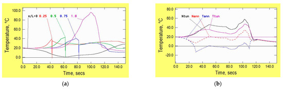
Figure 3.
Temperature histories in the tunnel and alongside the vehicle (base case), (a) tunnel, (b) vehicle. (x/L = proportional distance along tunnel. Ntun, Ttun = small distances ahead of the nose and behind the tail. Nann, Tann = in the annulus, small distances from the nose and tail).
After the vehicle has passed, there is again a loose resemblance with pressure trends, but the overall visual effect is less obvious because the strong discontinuity at the tail exists only for the static temperature, not for the stagnation temperature. Notwithstanding this distinction, it can be inferred from a comparison of Figure 2a and Figure 3a that temperature changes in each of the two main regions of flow are primarily due to pressure changes, not to thermal effects and entropy changes.
Broadly similar conclusions can be drawn from a comparison of pressures and temperatures at the chosen locations along the vehicle. Indeed, at the nose, the correlation is very close. At the tail, however, the differences between values in the annulus and behind the vehicle do not correlate with the corresponding pressure differences. Instead, they correlate quite well with the temperature differences at the nose (except for increased amplitudes). That is, the qualitative behaviour of the temperature is closely similar to that of an unchoked vehicle.
2.3. Velocity
Figure 4a shows air velocities in the tunnel and, once again, family resemblances with pressures can be seen. By inspection, however, some large velocities occur. It is obvious that this has to be the case relative to axes moving with the vehicle—because choked conditions imply air velocities equal to sonic velocities. However, it is somewhat less obvious relative to tunnel-based axes, although it is nevertheless easily understood. Indeed, even in main line railways, air velocities at some locations in tunnel systems can be as much as, say, 25% of the train speed despite the blockage ratios being considerably smaller than the 50% value in this base case.
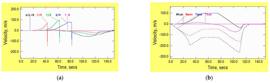
Figure 4.
Velocity histories in the tunnel and alongside the vehicle (base case), (a) tunnel, (b) vehicle. (x/L = proportional distance along tunnel. Ntun, Ttun = small distances ahead of the nose and behind the tail. Nann, Tann = in the annulus, small distances from the nose and tail).
The velocities shown in Figure 4b for the vehicle exhibit a number of revealing characteristics in addition to quantifying the venturi effect of the constriction caused by the vehicle. As a preliminary, however, it is emphasised that the graphs show velocities relative to the tunnel, not velocities relative to the vehicle. This is important information because it explains why the flow at the rear of the vehicle chokes when the depicted velocity is only about 200 m/s, but unchokes when it is closer to 300 m/s. At the first of these instants (about 30 s), the vehicle speed exceeds 100 m/s, so the relative velocity of flow approaching the geometrical discontinuity is well in excess of 300 m/s. In contrast, its speed at the instant of unchoking is only about 65 m/s. The velocity just behind the vehicle also merits attention. During the first 50 s or so, it is consistently positive, indicating that the mass of air in the expanding region behind the vehicle continually reduces in comparison with the ambient mass in the same region. This is consistent with the reducing pressure shown in this region in Figure 2a. For the remainder of the journey, the opposite behaviour exists. That is, the deficit is continually replenished, and the pressure increases for an extended period. It is informative to notice, however, that the pressure and temperature in this region remain greater than their ambient values long after the vehicle has stopped, and the air has become almost stationary. This indicates that some effect that has not been described above must exist and, in practice, this is a simple effect, namely an increase in specific entropy caused by (i) skin friction on the tunnel and vehicle surfaces, (ii) the choking at the tail of the vehicle and (iii) the reduction in stagnation pressure in the expansion of flow behind the vehicle. Another informative feature at the tail is the abrupt changes in sign of rates of change in velocity when the flow chokes and unchokes. For example, after choking occurs, the backflow relative to the vehicle cannot increase strongly and so the subsequent increase in vehicle speed until 50 s has elapsed necessarily causes the air along the annulus to accelerate in the same direction as the vehicle.
2.4. Mach Number
For completeness, Figure 5 shows Mach numbers relative to the vehicle. The key location is at the tail of the annulus, where the Mach number rises rapidly to one, remains in this choked condition for most of the journey and then falls rapidly to zero as the vehicle decelerates. The corresponding value just behind the nose has a broadly similar shape except that its maximum value is smaller. The dominant cause of these different maxima is the strong density gradient along the annulus, associated with the pressure gradient required to overcome frictional resistance. Since the mass flow rate varies only gradually along the annulus, the upstream velocity (relative to the vehicle) is smaller than the downstream value, whereas the sound speed is greater than the downstream value. Both of these contribute to the need for the Mach number to increase from the nose to the tail. Its value just ahead of the nose is less than half of the value at the front of the annulus, primarily because of the halving of flow area, but also because the upstream density is greater.

Figure 5.
Mach number relative to the vehicle.
- (Ntun, Ttun = small distances ahead of the nose and behind the tail.
- Nann, Tann = in the annulus, small distances from the nose and tail).
The shape of the history just behind the tail differs strongly from that at the other three locations. However, the difference is strong only during the period when the flow at the rear of the annulus is choked. Before and after that period, the histories ahead of and behind the vehicle are closely similar. The evident lack of a correlation of conditions across the tail is clear evidence of the partial de-coupling of the two regions of flow. Prior to (and after) the period of choked flow, waves travelling along the tunnel in either direction can cross the discontinuity. In the intervening period, however, waves travelling in the same direction as the vehicle cannot do so. Instead, they effectively see the discontinuity as a barrier at which, consequently, they will reflect almost totally. During this period, the mass flow rate relative to the vehicle is determined solely by the upstream conditions.
2.5. Drag and Power
Figure 6a shows the forces required to balance inertial (continuous line) and aerodynamic (broken line) resistance and Figure 6b shows the corresponding powers. In the chosen base case, the magnitudes of the aerodynamic component are almost negligible in comparison with the inertial component so, in the Figure, they are amplified by a factor of 50 to enable meaningful deductions to be made. However, care needs to be taken in the interpretation of the disparity in magnitudes because the net energy consumption for acceleration and deceleration is zero whereas that for the aerodynamic component is positive. If it is assumed that the power supply and regenerative braking are 100% efficient, then the only release of energy to the tunnel air will be due to the aerodynamic resistance. Indeed, this could still be the case even if the powers for propulsion and braking are not 100% efficient provided that the resulting waste energy is discharged outside the tunnel. In both cases, the residual increases in pressure and temperature after the vehicle has stopped will be due to the aerodynamic component.

Figure 6.
Power demand for inertial forces and aerodynamic drag (base case), (a) inertial and drag forces, (b) power demand. (K.E. = inertial component; Dg.50 = Drag component × 50).
Particular attention is drawn to the gradual increase in the drag force during the period when the vehicle is travelling at constant (and maximum) speed. This is a consequence of the continuously increasing difference between pressures ahead of and behind the vehicle during this period. It has important consequences for analysts using 3-D methodology with local boundary conditions that implicitly assume the existence of steady-flow conditions ahead of and behind the vehicle. The resulting analyses can be excellent predictors of instantaneous quasi-steady conditions, but the outcomes do not, by themselves, give information about which stages of the journey are most accurately represented. This ambiguity is encountered in Section 3.1.1, in which drag coefficients inferred from the present simulations are compared with published values from a 3-D CFD analysis.
For completeness, it is noted that no account is taken herein of heat sources such as
- Inefficiencies in the propulsion and braking systems;
- Sensible heat from passengers;
- On-board systems such as lighting and air management.
The potential of these to impact the conditions in the tunnel air will depend on the methods used to handle them. Nevertheless, it is likely that they will have only a small influence on vehicle temperatures and consequently on air temperatures too. A possible exception is mechanical braking in the event that this ever becomes necessary, but rare events such as this are out of the scope of this paper.
2.6. Numerical Accuracy
All predictions obtained using any numerical method of solution are approximate to some degree. Typical causes of error include (i) the applicability of the underlying equations, (ii) the numerical representation of the equations, (iii) numerical discretisation, and (iv) iteration convergence criteria. Each of these is considered in this Section.
2.6.1. Analytical Equations
The principal limitations of the governing equations are (i) the representation of flows using cross-sectional mean values and (ii) the use of empirical expressions to represent phenomena causing non-inertial changes in stagnation pressure, stagnation temperature and hence specific entropy. The first of these precludes detailed modelling of flows in locations where 3-D behaviour is significant—e.g., close to the noses of vehicles—and where the flow is greatly disturbed—e.g., in long-wake flows behind vehicles. Herein, as in most 1-D simulations, local changes in geometry are represented as abrupt discontinuities across which the flow satisfies quasi-steady expressions. Similarly, the chosen empirical expressions used to model skin friction and local pressure losses are strictly applicable only to quasi-steady flow conditions even though the author has devoted a significant part of his career to studying the limitations of such methods.
The equations are formulated using temperature, specific entropy and Mach number as the primary variables. Analytically, it would be equally suitable to use other combinations—e.g., pressure, temperature and velocity. However, for reasons presented by Vardy (2023) [13], the chosen combination is more suitable for use with the desired numerical methodology. In a nutshell, it enables a partial numerical de-coupling of phenomena propagating at particle speeds from phenomena propagating at wave speeds.
When the flow at the vehicle tail is choked, the change in stagnation pressure cannot be modelled by the empirical method described above. Instead, the conditions in the annulus just upstream of the tail are determined using (i) an MoC wave equation, (ii) an MoC path equation and (iii) the stipulation Ma = 1. This enables the determination of the mass flow rate and the stagnation temperature, both of which are assumed to be unchanged by the discontinuity. Conditions downstream of the tail region are obtained using these two parameters together with an MoC wave equation. This is considered adequate for the relatively long, uniform area vehicles considered herein, even though it might not be justified for short, longitudinally streamlined pods when supersonic flows exist.
2.6.2. Numerical Equations
The method used to represent the analytical equations numerically is the Method of Characteristics (MoC), which is widely used in studies of 1-D wave propagation. However, the most common applications are in low Mach number flows and/or in flows where the amplitudes of pressure changes are only a small proportion of the absolute pressures. As a consequence, it would not be safe to regard the excellent performance of the method in such applications as sufficient evidence to justify its use herein. Instead, as described in Appendix A, detailed comparisons made previously with a completely different method (finite volume) are cited for this purpose. The latter method has the advantage of avoiding a well-known limitation of MoC, but the disadvantage of not being targeted specifically at wave propagation.
2.6.3. Numerical Discretisation (Grid Size)
Two independent factors influence the most suitable grid size. The more obvious of them is the need to reduce differences between the numerical solution and the (unknown) analytical solution that the simulations are intended to replicate. In practice, the best that can be achieved in this respect is to obtain solutions for successively smaller grid sizes until differences between them are considered to be acceptably small. This is a necessary condition, although it does not, by itself, guarantee that the converged numerical solution is equivalent to the desired solution of the analytical equations. When practicable, independent comparisons with physical measurements or other methods of solution can reduce this uncertainty.
A second, less widely discussed issue relating to grid size is the detail in which the physical significance of converged solutions should be interpreted. Anyone using a 1-D method implicitly accepts that variations within flow cross-sections will be disregarded, even in the analytical equations. Likewise, they accept that simulated disturbances at geometrical “discontinuities” such as vehicle noses will be artificially foreshortened. It would be illogical to interpret the overall predictions in greater detail than is justified in the light of such approximations in the representation of the simulated phenomena.
As well as choosing the spatial grid size appropriately. Attention has to be paid to the temporal grid size. The chosen software automatically ensures that the integrations respect the Courant–Friedrichs–Lewy (CFL) stability criterion. Further, it includes algorithms that seek to minimize the consequences of interpolations that are inevitable when using the Method of Characteristics (MoC) for flows in which the speed of propagation of waves cannot reasonably be regarded as constant. A detailed discussion of the application of MoC to high Mach numbers is given by Vardy (2023) [13].
The graphs presented above have been obtained using a numerical grid length of 5 m, which corresponds to approximately 1½ tunnel diameters. This grid size has also been used for all subsequent simulations for the 15 km tunnel even though, with only one exception, only tiny differences exist from corresponding predictions using a grid length of 10 m. The single exception is a simulation with a vehicle length of 25 m. For this case, only two complete grid lengths of 10 m exist along the vehicle, and small, but clearly noticeable, differences exist from the presented solution using a 5 m grid length. In all other simulations, the vehicle length is equal to (or greater than) five 10 m grid lengths and hence ten 5 m grid lengths.
2.6.4. Convergence Tolerances
The underlying equations used herein are highly non-linear and it is necessary to solve several of them simultaneously. As a consequence, the use of iterative methods of solution is unavoidable and so convergence tolerances must be chosen. For simulations herein, the chosen tolerance for velocity is UOK = 10−4 and all other tolerances depend on this in internally prescribed manners. For completeness, it is declared that no differences have been detected from Figure obtained using tolerances of 10−3 and 10−5.
3. Sensitivity to Key Parameters
The detailed focus on a single case given in the preceding Section is supplemented in this Section by exploring the sensitivity to assumed values of various parameters whose values are necessarily system dependent. Consideration is given first to parameters that primarily dictate the overall force balance, then to parameters that primarily influence thermal phenomena, and finally to operational parameters. Of course, changes in pressure are inevitably accompanied by changes in temperature—and vice versa—and both cause changes in density and velocity. Nevertheless, the above distinctions are useful for understanding the governing mechanisms.
Throughout this Section, the specification of the tunnel remains as stated in Table 1. A much onger tunnel is considered in Section 4. It is emphasised that this is a sensitivity study, not a full parametric study. Each case in this Section varies in only one respect from the base case. Full design studies need to assess multiple combinations of values, but the trends to be expected can be inferred from sensitivity studies such as this, provided that the chosen base case is appropriate for the particular project.
3.1. Vehicle Parameters
3.1.1. Cross-Sectional Area
Figure 7a,b shows pressures along vehicles with cross-sectional areas of 2.5 m2 and 7.5 m2, respectively. By inspection, this has a huge influence on the pressures, especially on the maximum values ahead of the vehicle. There are two key reasons for this. The more obvious of the two is simply that increases in vehicle area correspond to decreases in the area available for flow along the annulus. This reduces the rate of backflow and hence increases the rate of flow driven ahead of the vehicle, thereby increasing the rate of compression in that region. The less obvious of the two key reasons is that the period during which choked flow exists increases with increasing vehicle area. For the three cases presented (areas of 2.5, 5.0 and 7.5 m2) the durations are approximately 37, 80 and 104 s, respectively. During these periods, the backflow along a vehicle scales approximately with density.
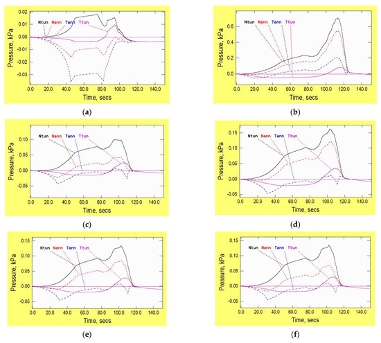
Figure 7.
Influence of vehicle parameters on pressures along it, (a) vehicle area = 2.5 m2, (b) vehicle area = 7.5 m2, (c) vehicle length = 25 m, (d) vehicle length = 150 m, (e) vehicle friction coefficient, fveh = 0.004, (f) vehicle nose coefficient = 0.2. (Ntun, Ttun = small distances ahead of the nose and behind the tail. Nann, Tann = in the annulus, small distances from the nose and tail).
In this description, changes in the vehicle:tunnel blockage ratio correspond to differing vehicle areas in a given tunnel. They could alternatively arise for a given vehicle in tunnels with differing areas. From such comparisons, it has been found that the correlations with blockage ratio are close, but not exact. Small differences exist as a consequence of Reynolds number effects that depend upon size as well as shape. Nevertheless, for initial design purposes in any study, it will be sufficient to focus on blockage ratios instead of assessing the vehicle and tunnel areas independently.
It is possible to compare data from these simulations with specific predictions from published 3-D CFD analyses when the latter are presented in aggregate forms devoid of 3-D details. Table 2 compares drag coefficients given by Bizzozero et al. (2021) [3] with corresponding values obtained from a series of simulations such as those presented in the base case and in the above figure. The chosen blockage ratios are those listed by Bizzozero et al., but the comparisons require interpolation from their data to give the vehicle Mach number used herein, namely 0.5825. This is the ratio of the vehicle speed (200 m/s) and the speed of sound in the ambient conditions (343.3 m/s). Table 2 by Bizzozero et al. includes data for vehicle Mach numbers of 0.5 and 0.6 so errors due to the interpolation will be quite small. For this purpose, the drag coefficient is evaluated as
where the suffices “amb” and “z” denote ambient conditions and the vehicle, respectively.
Table 2.
Vehicle drag coefficients: Instantaneous 1-D v. steady-flow 3-D.
Some warnings are necessary regarding any conclusions drawn from these data. First, although the comparisons are based on vehicles with the same maximum cross-sectional areas, their longitudinal profiles differ strongly, and this will necessarily influence conditions in the wakes behind them. It is to be expected that drag forces obtained by 3-D CFD for a vehicle of uniform cross-section would also differ from those for the shaped vehicle reported in Table 2. Second, data from Bizzozero et al. [3] are presented for an asymptotic state, whereas the 1-D data correspond to conditions that are evolving in time. The importance of this can be inferred from the proportional difference between conditions at the beginning and end of the period of constant speed. This proportion increases with the blockage ratio, thereby implying that the time required to approach asymptotic conditions also increases. As a consequence of these differences, it is not safe to make quantitative comparisons between the two sets of data. Nevertheless, they both confirm that the drag coefficient defined in Equation (1) itself increases strongly with the blockage ratio. Even when the ratio is as small as 0.2, the coefficient is significantly greater than unity. Further information about the influence of the evolving flow conditions is seen in the simulation of a longer tunnel in Section 4.
3.1.2. Length
Figure 7c,d show pressures along vehicles with lengths of 25 m and 150 m, respectively, namely half and three times the length in the base case. This causes only minor differences at the tail, but it strongly influences pressure changes along the annulus that are necessary to overcome skin friction resistance to backflows. This, in turn, causes larger pressures ahead of long vehicles than shorter ones, although the influence is far smaller than that of the blockage ratio. The maximum aerodynamic drag for the 150 m long vehicle is only about 50% greater than that for the 25 m vehicle and 33% greater than that for the 50 m vehicle (the base case). This is because form drag dominates skin friction drag along short vehicles (e.g., Oh et al. 2019 [14]. The implication is that, for a given passenger capacity, longer vehicles may be more power-efficient than shorter ones. It is shown later that this deduction remains valid even when several short vehicles travel in a convoy.
3.1.3. Skin Friction
Figure 7e shows pressures based on a doubling of the assumed vehicle skin friction coefficient of the base case vehicle to fveh = 0.004 (λveh = 0.016). This value is implausibly high for vehicles intended for use in evacuated tunnels, but it is useful for illustrating the influence of skin friction. For comparison, at the other extreme, implying a totally smooth vehicle surface, the coefficient would be approximately fveh = 0.0015 (λveh = 0.006). The doubling of the coefficient causes the pressure difference along the annulus to increase by approximately a third, but the peak pressure ahead of the nose increases less than half as much. Taken together with the above dependences on vehicle area and length, it may be concluded that, although the frictional resistance along the vehicle has a marked influence, it is much less important than the blockage ratio.
Although it is reasonable in principle to use quasi-steady approximations to model skin friction on vehicle surfaces, the use of coefficients such as those cited above is markedly less reasonable. The empirical formulae in which they are used are intended only for the case of regions of steady, fully developed, uniform flow—i.e., that are sufficiently long for the influence of disturbed inlet conditions to be neglected. However, errors arising from this cause are unlikely to be important, partly because they decrease with increasing vehicle length. Furthermore, detailed 3-D analyses such as those described by Braun et al. (2017) [7] and Opgenoord & Caplan (2018) [9] show that the skin friction component of drag on actual vehicles will be less strong than the pressure (form) drag component. Indeed, the transition from laminar to turbulent flow on the vehicle surfaces is likely to be induced prematurely for this very reason.
3.1.4. Nose Loss Coefficient
The influence of stagnation pressure losses at the vehicle nose is considered in a similar manner. That is, Figure 7f shows pressures based on an implausibly large value, namely 0.2, and a comparison with the base case shows that the consequences along the annulus are relatively minor. Even with such a large value, little influence is seen in conditions along the annulus or behind the tail. That is, the reduction in the rate of backflow caused by the nose loss has the counter consequence of slightly reducing the subsequent pressure gradient along the annulus. The maximum pressure ahead of the vehicle increases by about 20%. A realistic value of this coefficient for a reasonably designed vehicle would be much closer to the base case than to 0.2.
3.1.5. Tail Loss Coefficient
No figure is presented for the only remaining vehicle parameter in Table 1, namely the pressure loss coefficient at the tail. This is primarily because stagnation pressure losses due to this cause are dwarfed by the change caused by the choking of the flow. However, even in the periods before and after choking, the influence is weak over a wide range of plausible values (namely zero to 2βz2). The lower end of this range would imply perfect streamlining enabling the flow behind the tail to expand without causing a wake. The upper end is twice the value that would pertain to a blunt-ended train on a conventional railway. This doubling would be implausible during sub-sonic periods of flow, although it may be possible in principle when the flow is choked because the expansion could then involve a succession of oblique shocks that reflect at the walls of the tunnel and form a diamond-shaped pattern wake region.
It is assumed herein that the vehicle designers will ensure sufficient streamlining to avoid tail losses as large as the upper end of the stated range in subsonic flows. For completeness, however, it is noted that, in principle, losses at the tail could have a decisive influence if they were much greater than the assumed range. With unusually strong losses, the critical location for flow control could pass from the rear of the annulus to behind the tail and the whole flow pattern would then change. That is, the flow in the annulus would remain subsonic and choking would occur instead in the tunnel behind the vehicle. This has the potential to increase the aerodynamic drag strongly, so it is unlikely to be an acceptable operating condition unless the ambient pressure is very low.
3.2. Thermodynamic Influences
The vehicle parameters considered in the preceding Section primarily influence forces. Attention now turns to parameters that primarily influence temperatures. In all cases, changes in either of these induce changes in the other, but the drivers are nevertheless fundamentally different. More importantly, however, the most suitable values of all of the parameters considered in this Section are strongly system dependent and some of their inferred influences can vary strongly with the time scales over which they are assessed. These can range from seconds or minutes to years or decades. Herein, only the shorter time scales are considered.
3.2.1. Heat Transfers at Tunnel and Vehicle Surfaces
Perhaps the most important item in this category is heat transfer with the surfaces of the vehicle and tunnel. Two phenomena contribute, namely (i) convective heat transfer between the air and the surfaces and (ii) heat conduction within the surrounding material. The evolving surface temperatures are determined by a balance between these two. This is achieved in the software by solving equations for the two phenomena simultaneously. At both surfaces, convection coefficients are estimated using the Reynolds analogy for quasi-steady flows. The methods used to represent conduction within the tunnel and vehicle walls are different. Transient heat conduction equations are solved in the tunnel walls, assuming uniform wall properties, but a lumped thermal mass approximation is used to represent the vehicle. The principal reason for using different approaches is that the numerical grids in the air and the wall are fixed relative to the tunnel. Accordingly, no interpolation is required in communication between them. In contrast, this is not possible on the surfaces of vehicles that are moving along the tunnel. This is a decisive matter because the evaluation of information at fixed locations along a vehicle would necessarily involve interpolations. Errors due to this cause would interact with time-dependent quantities and, at best, make the solutions unreliable.
It is far from certain that significantly better predictions would be obtained from typical 3-D software even though the use of sliding grids would be likely to reduce interpolation issues by moving the location of interpolations away from the surface. However, the detailed determination of convection coefficients depends on the choice of turbulence models and this challenge has not been fully mastered even for skin friction coefficients, let alone heat transfer coefficients (see Gorji et al. 2014 [15], for instance). Relatively few turbulence models make satisfactory allowance for rapidly accelerating flows and even fewer can do so when the same simulation also includes extensive regions of slowly varying flows.
In practice, in the time scales of single journeys that are the focus herein, the expected rates of heat transfer will induce only small changes in surface temperatures of either the tunnel or the vehicles. This is because (i) the air density is small so the associated heat transfer coefficients are small and (ii) the thermal capacitances of the tunnel and vehicle are much larger than that of the air. Accordingly, it will normally be acceptable to regard the surface temperatures as constant. In contrast, however, the small density also implies small thermal capacitance and so the small heat transfers can potentially cause large changes in air temperature, albeit over larger time scales than those associated with the dominant pressure changes. This is illustrated in Figure 8, which compares the base case with alternative simulations in which at least one of the surfaces is treated as adiabatic. By inspection, this has a strong influence on the shapes of the temperature histories as well as on the maximum values. The differences increase with increasing time because (i) the time available for heat transfers to occur with the tunnel wall before the vehicle arrives increases with increasing time, (ii) the influence of heat transfers is cumulative, and (iii) the dominant direction of heat transfer is from the air to the surfaces.

Figure 8.
Influence of convective heat transfer on temperatures along vehicle, (a) tunnel temperatures: Qtun = 0; Qveh = 0, (b) vehicle temperatures: Qtun = 0; Qveh = 0, (c) tunnel temperatures: Qtun > 0; Qveh = 0, (d) vehicle temperatures: Qtun > 0; Qveh = 0, (e) tunnel temperatures: Qtun = 0; Qveh > 0, (f) vehicle temperatures: Qtun = 0; Qveh > 0, (g) tunnel temperatures: Qtun > 0; Qveh > 0, (h) vehicle temperatures: Qtun > 0; Qveh > 0. (Ntun, Ttun = small distances ahead of the nose and behind the tail. Nann, Tann = in the annulus, small distances from the nose and tail).
The top row of the figure shows conditions when heat transfers are suppressed at both surfaces. In this idealised condition, the maximum temperature just ahead of the train is in excess of 100 °C and those further along the tunnel are even larger. In contrast, when heat transfers with the tunnel wall are modelled (Figure 8c,d), the corresponding values are much smaller. The contrast between Figure 7b,d is especially strong in the vehicle because of the time available at any particular location for heat transfers to occur before the arrival of the vehicle. The influence of heat transfers at the vehicle surface is much weaker than that of heat transfers at the tunnel wall. This can be inferred from comparisons of either the first and third rows of the figure or the second and fourth rows. A direct consequence is an increase in the temperature difference along the annulus (compare the two broken lines between about 90 and 100 s). An indirect consequence arises from the density increase that is associated with the reduced temperature. This increases the rate of backflow along the annulus and hence reduces the pressures and temperatures ahead of the vehicle. The net effect is small, but it is helpful, nonetheless.
3.2.2. Other Causes of Heat Transfers
Inefficiencies in propulsion and braking systems can induce significant heat transfers in tunnels on conventional railways. In the case of high-speed passenger trains, however, the consequential temperature variations over short time scales are typically quite small because the relative air velocities are large, and the specific thermal capacity of the air is a thousand times greater than that in the evacuated tunnel under consideration herein.
In the present case, the strong pressurisation of air ahead of a vehicle causes the temperature of the air entering the annulus around it to be high and so heat transfers with the vehicle will normally be from the air to the vehicle. Even if transfers in the opposite direction were to occur, quite small heat releases from the vehicles could rapidly cause temperatures of the low-density air to approach those of the vehicle surface, thereby suppressing subsequent transfers. It follows that waste energy from propulsion and braking processes cannot normally be discharged passively into the tunnel (although braking in the event of power failure will need to be considered). As a consequence of this line of reasoning, another parameter that does not need to be considered in relation to energy transfers with the air is the vehicle mass, even though this has a dominant influence on power flows during acceleration and deceleration.
Similar arguments apply to the equivalent of what is known in conventional railways as rolling resistance. In the case of levitated vehicles, the equivalent phenomenon will be enhanced skin friction in the neighbourhood of the guiding surfaces. For the purposes of the present paper, it is not possible to distinguish these meaningfully from the overall skin friction considered in Section 3.1.3. However, since the focus in this Section is on energy rather than on forces, it is perhaps worth pointing out that friction is essentially a force and that its consequences for energy transfers arise from considerations of work, not heat. Such reminders are commonly regarded as pedantic, but they are important for overall understanding, and they are especially pertinent in cases such as evacuated tunnels where the opportunity for temperature-driven energy release into the air may not exist.
3.3. Operational Considerations
Consideration is now given to three parameters that, at least in principle, could be varied in an operational system, namely (i) the ambient pressure, (ii) the vehicle speed history and (iii) the number of vehicles travelling simultaneously. Each of these could have a major influence.
3.3.1. Ambient Pressure
In Figure 9a, the ambient pressure is 1 kPa—i.e., ten times greater than in the base case. This is still only 1% of the atmosphere, so it is a plausible option. The resulting temperatures and velocities differ relatively little from the base case, but (i) pressure-changes and (ii) the air density increase by factors of approximately ten—i.e., broadly in proportion to the increase in ambient pressure. Perhaps the most significant change is a ten-fold increase in the power required to overcome aerodynamic resistance (Figure 9b). The maximum value is about 20% of the maximum needed for the prescribed vehicle acceleration. The graph is amplified by a factor of 5, whereas the corresponding graph in Figure 6b is amplified by a factor of 50.

Figure 9.
Influence of ambient pressure on vehicle pressures and power, (a) inertial and drag forces, (b) power demand. (Ntun, Ttun = small distances ahead of the nose and behind the tail. Nann, Tann = In the annulus, small distances from the nose and tail. K.E. = inertial component. Dg.5 = drag component × 5).
3.3.2. Vehicle Speed History
Figure 10a illustrates consequences of a possible alternative speed history in which the maximum speed is unchanged, but the acceleration and deceleration are increased from 4 m/s2 to 5 m/s2. This increases the magnitudes of inertial drag and power flows, although the net energy consumption for this purpose is still zero (on the assumption of 100% efficiency). The energy consumed to overcome air resistance (friction and inertia) increases, but by only a few percent. The practical benefit of the increased acceleration is a small reduction in journey time. This reduction is independent of the tunnel length so its operational value will decrease with increasing length.
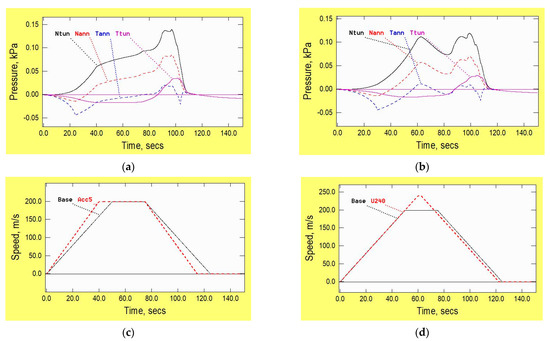
Figure 10.
Influence of vehicle speed history on pressures along it, (a) acceleration = 5 m/s2, (b) maximum speed = 240 m/s, (c) speed history, (d) speed history. (Ntun, Ttun = small distances ahead of the nose and behind the tail. Nann, Tann = in the annulus, small distances from the nose and tail).
In longer tunnels, a more significant reduction in travel time can be obtained with the original accelerations, but an increased maximum speed (Figure 10b). This is effective for all tunnel lengths in which the increased speed is reached before deceleration commences. The consequential reduction in journey time increases with increasing tunnel length, but so does the energy required to overcome flow resistance. Although the latter is unimportant in short tunnels, it could be a relevant consideration in much longer tunnels. Naturally, however, the maximum power requirement during acceleration and deceleration is increased, as is the power required to overcome aerodynamic resistance. Likewise, the overall energy consumption to overcome the flow resistance increases. In the base case tunnel, an increase in maximum speed to 240 m/s at 0.4 m/s is only just achievable. The durations of acceleration and deceleration are 60 s and the duration at maximum speed is only 2.5 s. The two alternative speed histories are shown in Figure 10c,d together with the corresponding base case history and the influence of vehicle speed is reconsidered in Section 4 for a longer tunnel.
3.3.3. Number of Vehicles
In tunnels of sufficient length, it will be common for more than one vehicle to be travelling at any given time. The actual number and the intervals between vehicles will vary according to demand, and many combinations will need to be assessed during practical design studies. Herein, just one case is considered. At time zero, there are three stationary vehicles, separated by gaps of 25 m. Their noses are, respectively, 250, 175 and 100 m from one end of the tunnel. The second and third vehicles begin their journeys 10 s and 20 s after the first.
Although a detailed investigation of the interactions between each vehicle would not be practicable, useful information can be deduced from comparisons of the pressures and velocities along the individual vehicles. In Figure 11, the upper, middle and lower rows relate to the first, second and third vehicles, respectively. The equivalent histories for a single vehicle are in Figure 2b and Figure 4b. These Figures can be used to assess the significance of a vehicle’s location within a group.
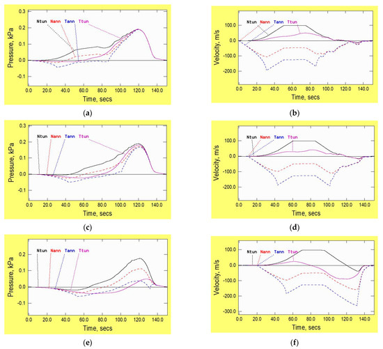
Figure 11.
Influence of position in convoy on flow conditions (single tunnel), (a) pressures along leading vehicle, (b) velocities along leading vehicle, (c) pressures along middle vehicle, (d) velocities along middle vehicle, (e) pressures along trailing vehicle, (f) velocities along trailing vehicle. (Ntun, Ttun = small distances ahead of the nose and behind the tail. Nann, Tann = in the annulus, small distances from the nose and tail).
Interactions between the three vehicles are especially pronounced in the velocity histories. In common with the single-vehicle case, the velocity behind the tail (Tann) of the third vehicle shows strongly increasing backflow during, and after, the period of choking. This contrasts sharply with the histories behind the first two vehicles. It is a consequence of the fact that the first two vehicles are helped by following vehicles during the later stages of their journeys whereas the third is not. The influence of mutual help is also seen in the much-reduced durations of periods of choked flow along the first and second vehicles in comparison with the third.
The different consequences of mutual help are also seen in the pressure histories. Alongside the first vehicle, for instance, the pressures are initially similar to those for a single vehicle, whereas, in later stages of the journey, they are very different—because this vehicle is in the region of high pressure induced ahead of the following vehicles. In contrast, for the third vehicle, strong differences exist in the early stages, whereas those in the later stages are much less pronounced.
Informative comparisons can be made between the aerodynamic drag forces on the three vehicles with the corresponding force for a single vehicle with the same overall length of 150 m (pressures for the latter are presented in Figure 8d above). Table 3 shows the peak values of drag force and power demand for each vehicle together with the total energy consumption during the simulated period. Perhaps the most striking single result is the fact that the maximum drag force on the trailing 50 m vehicle exceeds that on the single 150 m vehicle. However, this has a simple explanation. The leading two vehicles cause a strong accumulation of mass ahead of them whilst their tails are choked. The release of this mass when the second vehicle unchokes exposes the trailing vehicle to a strong headwind. This exists only during the later stages of the journey after the trailing vehicle has begun to decelerate and after the time of maximum power demand. The maximum forces and power demands on the leading two vehicles are much smaller than on the trailing vehicle, and so are their total energy consumptions. In this short tunnel, the combined energy consumption for the three shorter vehicles is almost 75% greater than that for the single longer vehicle, and this has obvious implications for overall system running costs.
Table 3.
Energy consumption to overcome aerodynamic resistance.
For completeness, it is pointed out that the relative importance of the early and late periods is a function of the tunnel length. In all examples discussed so far, the vehicles spend far more time accelerating and decelerating than they spend at maximum speed—e.g., 50 s, 25 s and 50 s in the base case. In a tunnel that is twice as long, the corresponding values would be 50 s, 100 s and 50 s. Of course, the number of vehicles in motion at any one time may also vary with the tunnel length.
4. Longer Tunnels
The base case tunnel is shorter than the lengths commonly envisaged in studies of high-speed vehicles in evacuated tunnels. To assess the importance of this, Figure 12 compares the vehicle pressures, temperatures and power requirements in the base case tunnel and in a tunnel that is four times as long. The only other change from the base case is the duration of travel at maximum speed. In the longer tunnel, the vehicle accelerates for 5 km, travels at constant speed for 50 km and then decelerates for 5 km. The additional 45 km at 200 m/s increase the journey time by 225 s to a total of 350 s.
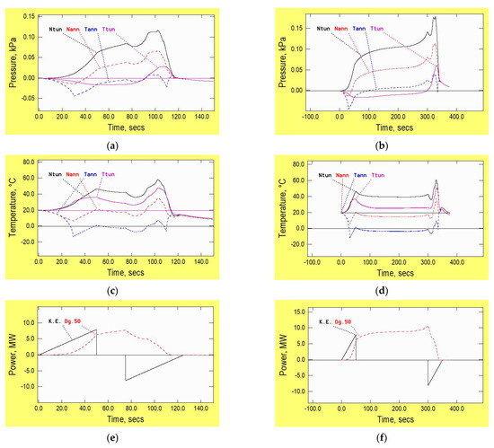
Figure 12.
Influence of length of tunnel, (a) pressure along vehicle: 15.4 km tunnel, (b) pressure along vehicle: 60.4 km tunnel, (c) temperature along vehicle: 15.4 km tunnel, (d) temperature along vehicle: 60.4 km tunnel, (e) vehicle tractive power: 15.4 km tunnel, (f) vehicle tractive power: 60.4 km tunnel. (Ntun, Ttun = small distances ahead of the nose and behind the tail. Nann, Tann = in the annulus, small distances from the nose and tail).
The conditions in the two tunnels during the early stages of the journey are identical. No difference is possible until reflections begin to arrive at the vehicle from the distant end of the tunnel, namely at approximately 30 s in the case of the 15.4 km tunnel. Likewise, conditions in tunnels longer than 60 km would be identical to those in the 60.4 km tunnel throughout the first two minutes of the journey. After the arrival of the first reflections, the rate of increase in pressure ahead of the vehicle nose increases and, during the period of constant vehicle speed, the rate is greater in the shorter tunnel than in the longer one. Thereafter, the pressure ahead of the vehicle in the longer tunnel continues to increase and the eventual maximum value exceeds that in the shorter tunnel by about 50%.
In both tunnels, the vehicle temperatures vary relatively slowly during the period of constant vehicle speed. They then decrease for a short period before increasing strongly as the vehicle approaches the closed end of the tunnel. Short-term changes in temperature approximately mirror those for pressure, although sustained heat transfers at the tunnel wall gradually counter the changes over long periods.
The aerodynamic drag force and consequential tractive power requirement depend strongly on the difference between pressures ahead of and behind the vehicle. In both tunnels, these values increase slowly, but continually, throughout the period at constant vehicle speed and the maximum value in the longer tunnel is about 35% greater than that in the base case tunnel.
Influence of Vehicle Speed
In sufficiently long tunnels, it is possible to assess the dependence on vehicle speed more fully than was possible with the shorter tunnel considered in the base case. Figure 13 shows pressures and temperatures in a 30.4 km tunnel for vehicles travelling at 150, 200 and 250 m/s between periods of uniform acceleration and deceleration of 4 m/s2. The overall journey times for these cases are 237.5, 200.0 and 182.5 s, respectively. During most of the periods of steady speed, the pressures scale approximately with the square of the vehicle speed. In the later stages of the journey, however, the behaviour differs strongly from this. Indeed, the maximum pressures are almost the same in all three cases. During this period, therefore, the influence of the vehicle speed is secondary to the influence of choking and its consequences for the achievable rates of backflow along the vehicles. A broadly similar outcome is also seen for temperatures provided that attention focuses on differences from ambient conditions, not on absolute values.
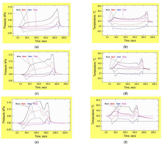
Figure 13.
Influence of vehicle speed (30 km tunnel), (a) vehicle pressures: 150 m/s, (b) vehicle temperatures: 150 m/s, (c) vehicle pressures: 200 m/s, (d) vehicle temperatures: 200 m/s, (e) vehicle pressures: 250 m/s, (f) vehicle temperatures: 250 m/s. (Ntun, Ttun = small distances ahead of the nose and behind the tail. Nann, Tann = in the annulus, small distances from the nose and tail).
5. Alternative Tunnel Configuration
In practical systems, there will commonly be two tunnels—one for each direction of travel. In this case, designers will need to decide whether these should be aerodynamically separate or should be connected in some manner. One obvious possibility is to link the tunnels at their ends, thereby causing them to act aerodynamically as a single continuous loop (Figure 14). In this case, all vehicles will tend to cause the air to circulate in a common direction. This has the twin advantages of (a) increasing the number of vehicles that provide mutual help and (b) removing the closed-end effect that is responsible for the strong pressurisation at the end of a single tube.

Figure 14.
Aerodynamically linked tunnels for two-way operation.
Figure 15 shows pressure and air velocity histories for a twin tunnel system that is connected in this way. For simplicity, the connections are at the extreme ends of the tunnels, and they have the same cross-sectional area as the tunnels. The actual geometry in any real system will be less simple, partly because of the need to make provision for embarking and disembarking, but also for many other reasons. However, the aerodynamic consequences are unlikely to depend strongly on the particular geometry. Indeed, it will be a design requirement to prevent significant divergence from the ideal behaviour.
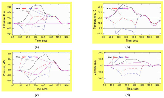
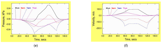
Figure 15.
Influence of position in convoy on flow conditions (linked tunnels), (a) pressures along leading vehicles, (b) velocities along leading vehicles, (c) pressures along middle vehicles, (d) velocities along middle vehicles, (e) pressures along trailing vehicles, (f) velocities along trailing vehicles. (Ntun, Ttun = small distances ahead of the nose and behind the tail. Nann, Tann = in the annulus, small distances from the nose and tail).
In the case considered in Figure 15, there are three vehicles in each direction, and, in each tube, the specified journeys are identical to those considered in Figure 11 for a single tube. When the vehicles begin to move, they generate pressure disturbances in both directions. In the single-tube cases, the influence of waves propagating in the same direction as the vehicles is dominant. In the twin-tube system, however, waves propagating in the opposite direction can have a stronger influence on the outcomes. This is a consequence of the time taken for waves to travel. First, consider a wave propagating ahead of the first vehicle to begin its journey. This will reach the remote end of the tunnel after about 45 s and it will then begin to travel along the second tube. By that time, however, the vehicles in the second tunnel will already have moved several kilometres and will be accelerating rapidly. As a consequence, an additional period of more than 5 s will elapse before the wave reaches the tail of the trailing vehicle. Furthermore, these times relate only to the tip of the wavefront. Much greater times will elapse before the arrival of the strongest parts of the wavefront. By that time, the leading vehicles will already be decelerating.
Now consider a wave travelling in the opposite direction to the vehicles. The leading tip of the wave initiated when the first vehicle begins to move will reach all three vehicles in the second tube before it reaches the remote end of that tube. Thus, it will begin to “assist” these vehicles before waves travelling in the same direction as the vehicles can do so. Of course, it is the overall influence of all waves that matters, not the contributions of individual waves, but this discussion illustrates the importance of taking account of waves circulating in both directions around the overall tunnel loop. Also, since the overall phenomenon is not fundamentally dependent on the number of vehicles, it may be concluded that the overall energy consumption can be reduced by coordinating the scheduling of journeys in the two tubes. This may be of relatively low importance in highly evacuated systems, but it will influence the selection of the most suitable ambient pressures.
The maximum pressures in Figure 15 ahead of the vehicle noses are only about a third of the corresponding values in an isolated tunnel (Figure 11). However, the reduction in the overall aerodynamic drag is much smaller than this. For the first and second vehicles, the overall energy consumption has reduced by about 20% and for the trailing vehicles it has reduced by about 40%. An important part of the reason for this can be inferred from the velocity histories along the vehicles and, in particular, from the durations of the periods of choked flow. By inspection, the reduction in the duration for the trailing vehicle is much greater than the reduction for the preceding vehicles.
6. Other Aerodynamic Considerations
Although this paper focuses almost exclusively on airflows generated by vehicle movements, many other factors will need to be considered in practical designs and some of these could be far more important than more obvious aerodynamic considerations. For completeness, a brief mention of a selection of such factors follows.
6.1. Response to System Power Failure
In the event of total loss of propulsive power, vehicles could become stranded and, if the situation were to persist for too long, the need could arise for re-pressurisation of a tunnel. The system will have been designed to ensure that the probability of such action becoming necessary is extremely small, but account nevertheless needs to be taken of the potential risk. Perhaps unexpectedly, this can be a reason for favouring very low ambient pressures. To illustrate this, suppose that the initial pressure is 5% of an atmosphere and that a safety issue requires this to be increased rapidly to one atmosphere. Further, suppose that the pressurisation will be undertaken longitudinally. In this case, the process will result in two regions of flow, namely (i) more than 5% containing primarily the original air and (ii) the remainder containing the newly supplied air. Thermodynamic considerations show that the temperature of the newly supplied air would be approximately the same as that of its source, but that the temperature of the original air would be hugely greater. In the limiting case of reversible, adiabatic compression, its absolute temperature would increase by a factor of about 2.3. The lower the ambient pressure, the smaller the mass of air to be re-pressurised and the smaller the region that it will occupy after re-pressurisation, but the greater the potential increase in temperature. It would be essential to plan procedures so that either (i) this air is constrained to a location where the effect can be tolerated or (ii) the re-pressurisation process is designed to mitigate its consequences.
6.2. Loss of Vehicle Sealing
In principle, the consequences of a loss of sealing of a vehicle could also escalate until re-pressurisation becomes necessary, leading to the effect just described. Once again, this risk can be made very small by proper vehicle design and airline-like initial responses, but it is nevertheless prudent to be aware of potential consequences in the event of such a situation developing.
6.3. Tunnel Wall Temperatures
The lower the ambient air pressure in the tunnel, the lower the capacity of the air to absorb energy. Even with large air velocities along the tunnel, convective heat exchanges with the tunnel wall are likely to be relatively small. The greatest values would probably be heat transfers into the wall during periods of especially high internal pressure, but even these rates will be small. It follows that the wall temperature is likely to depend much more strongly on external conditions than on internal ones. In the case of overland tubes in countries with hot climates and extensive periods of direct exposure to hot sun, the ambient air temperatures in the tunnels could be much greater than those assumed in the above simulations. In such cases, subsequent increases in temperature as a consequence of increased pressures would also be significantly higher.
6.4. Open Connections between Tunnels
In common with conventional railways, the advantages of any open connections between adjacent tunnels need to be weighed against other factors such as the need for total separation in the immediate aftermath of certain types of incidents. To achieve this, it might be necessary to ensure that the openings can be closed rapidly—possibly within less than a minute. In the event of this being necessary during an event that triggers re-pressurisation, it should be completed as early as possible because forces on closing doors could become excessive during later stages of closing.
6.5. Stations
Many different configurations of stations are possible. In some, the vehicles could remain in the main tunnel whereas, in others—especially stations at intermediate locations along a route—branched tunnels will be necessary to avoid disruption to non-stopping vehicles. In all cases, a key design objective will be to minimise the risk of significant amounts of air escaping into the tunnels. This will be important because of the high cost of evacuating tunnels. For the purposes of the present paper, however, it is the potential need for branching that matters because this has not been considered. The need can arise because of the large times required for deceleration and acceleration into and out of a station. These could have major consequences for vehicle schedules if stopping vehicles were in the same tube as non-stopping vehicles. In systems where a need for intermediate stations exists, this topic will merit dedicated studies of alternative geometrical configurations. However, the purposes of the present paper are best served by focussing on a single tunnel (or twin-tunnel loop) connecting just two stations. In this case, the need for parallel tunnel configurations for vehicles travelling in the same direction does not arise.
6.6. Other Factors
The above examples are far from exhaustive. Their purpose is simply to indicate that airflows caused by vehicle movements are only one consideration, albeit a potentially important one. Designers will also need to address many other factors such as, for instance, the cooling of vehicles that do not cool themselves in manners that are common in conventional railways (e.g., by convection to external air). Even though convection from tunnel air to vehicles will be small, the need for cooling will arise from sensible heat from passengers and from onboard equipment and lighting, etc.
7. Summary and Conclusions
The influence of a wide range of parameters on aerodynamic conditions in an evacuated tunnel conveying extra-high-speed vehicles has been studied. To avoid unnecessary complexity, the tunnel used in most of the study has been a single tube that is closed at both ends. Likewise, most of the comparisons have been based on the travel of a single vehicle. This simple combination has been sufficient to demonstrate the dominant role that can be played by the choking of flow at the rear of the annulus alongside a vehicle. For any particular ambient pressure in the tunnel, this is a strong determinant of the mass flow rate along the tunnel. The vehicle gradually compresses the air ahead of it to much larger proportional pressure changes than those in conventional railway tunnels. For instance, with a vehicle:tunnel blockage ratio of 0.5 travelling at 200 m/s, the maximum pressure ahead of the vehicle is more than double the ambient pressure.
Because the process is rapid, the increased pressures are accompanied by strong increases in temperature. For the same blockage ratio and vehicle speed, sustained temperatures just ahead of the vehicle can be around 60 °C and peak temperatures at the end of a closed tunnel can reach around 100 °C. However, these decay strongly because of heat transfers with the tunnel walls, albeit much more slowly than the initial increases caused by pressure waves.
It has been shown that the vehicle:tunnel area blockage ratio has a much stronger influence on pressures and temperatures than factors such as skin friction at the vehicle and tunnel surfaces or stagnation pressure losses at the vehicle nose.
The power required to overcome aerodynamic drag for a long vehicle is much smaller than for multiple shorter vehicles of the same overall length. Nevertheless, if multiple short vehicles are chosen (for operational reasons, say), there will be an advantage in operating them in discrete convoys—to maximise the periods of travel when they provide mutual assistance. For similar reasons, if adjacent tubes exist—e.g., for opposite directions of travel—it is beneficial to link them aerodynamically. This increases the number of vehicles providing mutual assistance and thereby reduces both the maximum power demand and the overall energy consumption. Furthermore, it greatly reduces the maximum pressure ahead of vehicles stopping at the end of a tunnel.
A brief mention has been made of various aerodynamic phenomena that have not been assessed quantifiably in this paper. In particular, attention has been drawn to the potential for the development of short regions of extremely large temperatures in the event of a need to re-pressurise an evacuated system rapidly.
Funding
This research received no external funding.
Data Availability Statement
Not applicable.
Conflicts of Interest
The author declares no conflict of interest.
Appendix A. Theoretical Basis
All simulations have been undertaken using the 1-D software package ThermoTun/8.1 (2022) [12], which is used in many countries for the assessment of railway tunnel aerodynamics, especially for high-speed railways. For such tunnels, it has had extensive validation, including comparisons with detailed measurements at full-scale and at model-scale. Even more important for the present author, all critical components of the software have been validated by comparisons with analytical solutions for idealised geometries. The equations of 1-D wave propagation in ducts have been known for more than two centuries and have been reported extensively. Accordingly, no useful purpose would be served by presenting them here. Any reader who is not already familiar with them could usefully consult a definitive book on compressible flow by Shapiro (1953) [16]. Likewise, Wylie and Streeter (1993) [17] give an excellent introduction to the basis of the Method of Characteristics and its use for simulating unsteady flows in pipes. The particular formulation of the underlying equations that are used in the software is based on the method recommended and explained by Vardy (2023) [13].
In common with most uses of 1-D methods (whether analytical or numerical), the software takes no account of the consequences of velocity variations within flow cross-sections. Also, it relies on user-specified coefficients to model phenomena such as skin friction and local losses of stagnation pressure. Furthermore, these coefficients are used in empirical expressions that are more suitable for some types of flow than others. For instance, in the simulations presented herein, the expressions used to model skin friction are based on quasi-steady flows. For completeness, it is worth pointing out that similar issues arise in relation to turbulence models in 3-D software and this can limit their reliability in studies of unsteady flows, especially in long ducts.
ThermoTun has three, wholly independent calculation modules with successively greater scope. The simplest is suitable at moderate Mach numbers provided that the relationships between changes in pressure and density approximate adequately to isentropic—as is the case in most tunnel designs. The second module takes account of heat transfers. It is suitable for greater Mach numbers than the first, but it loses accuracy when these exceed about 0.6. The third module, which is the one used herein, is a recent development. It is suitable for Mach numbers up to unity, but it is significantly more expensive in terms of CPU time (albeit still hugely less so than 3-D methods).
As declared in the main body of the paper, other 1-D software could be used. A particular example is NUMSTA (2019) [18] which was originally developed with funding from the Swissmetro project and was used extensively in that context. Its numerical algorithms are based on control volume analysis, whereas ThermoTun uses the Method of Characteristics. Advantage was taken of this fundamental difference in a paper that illustrated the influence of different aspects of compressibility in the context of railway tunnels (Vardy et al., 2009 [19]). The fact that the two complementary methods gave closely similar results up to Mach numbers of about 0.8 was taken as strong support for the predictions presented in that paper. At greater Mach numbers, both methods exhibited instabilities, and this subsequently became a motive for developing the third calculation method in ThermoTun. It remains stable up to a Mach number of unity and, thereafter assumes choked flow conditions.
For completeness, it is emphasised that nothing herein should be taken as formal validation of any particular methodology. Nevertheless, detailed (but unpublished) comparisons with analytical predictions give the author confidence in both of the stated software packages. They provide meaningful circumstantial evidence that the predictions in this paper will, at the very least, be reliable indicators of the relative importance of the many variables considered.
References
- Niu, J.; Sui, Y.; Yu, Q.; Cao, X.; Yuan, Y. Aerodynamics of railway train/tunnel system: A review of recent research. Energy Built Environ. 2020, 1, 351–375. [Google Scholar] [CrossRef]
- Kauzinyte, G.; Vezza, M.; Alizadeh, S.; Eckford, D. Hyperloop: Simulation and assessment of high-speed vehicle transport in evacuated tubes. In Proceedings of the 18th International Symposium on the Aerodynamics, Ventilation and fire in Vehicle Tunnels, Athens, Greece, 25–27 September 2019; Aini, E., Ed.; BHR Group: Bedfordshire, UK, 2019; pp. 61–76. [Google Scholar]
- Bizzozero, M.; Sato, Y.; Sayed, M.A. Aerodynamic study of a Hyperloop pod equipped with compressor to overcome the Kantrowitz limit. J Wind. Eng. Ind. Aero. 2021, 218, 104784. [Google Scholar] [CrossRef]
- Museros, P.; Lázaro, C.; Pinazo, B.; Monleόn, S. Key aspects in the analysis and design of Hyperloop infrastructure under static, dynamic and thermal loads. Engrg. Struct. 2021, 239, 112177. [Google Scholar] [CrossRef]
- Nick, N.; Sato, Y. Computational fluid dynamics simulation of Hyperloop pod predicting laminar-turbulent transition. Rail. Eng. Sci. 2020, 28, 97–111. [Google Scholar] [CrossRef]
- Tudor, D.; Paolone, M. Operational-driven optimal-design of a hyperloop system. Transp. Eng. 2021, 5, 100079. [Google Scholar] [CrossRef]
- Braun, J.; Sousa, J.; Pekardan, C. Aerodynamic Design and Analysis of the Hyperloop. AIAA J. 2017, 55, 4053–4060. [Google Scholar] [CrossRef]
- Chen, X.; Zhao, L.; Ma, J.; Liu, Y. Aerodynamic simulation of evacuated tube maglev trains with different streamlined designs. J. Mod. Transp. 2012, 20, 115–120. [Google Scholar] [CrossRef]
- Opgenoord, M.M.J.; Caplan, P.C. Aerodynamic design of the hyperloop concept. AIAA J. 2018, 56, 4261–4270. [Google Scholar] [CrossRef]
- Zhang, Y. Numerical simulation and analysis of aerodynamic drag on a subsonic train in evacuated tube transportation. J. Mod. Transp. 2012, 20, 44–48. [Google Scholar] [CrossRef]
- Swissmetro. Swissmetro Main-Study-1994–1998. 1999. Available online: https://swissmetro-ng.org/wp-content/uploads/Swissmetro-Main-Study-1994-1998-Level-A.pdf (accessed on 9 June 2023).
- ThermoTun. 2022. Available online: www.ThermoTun.com (accessed on 9 June 2023).
- Vardy, A.E. On the method of characteristics in highly compressible flows. In Proceedings of the 14th International Conference on Pressure Surges, Eindhoven, The Netherlands, 12–14 April 2023; Jones, S., Ed.; Tech Univ Eindhoven: Eindhoven, The Netherlands, 2023; pp. 443–457. [Google Scholar]
- Oh, J.-S.; Kang, T.; Ham, S.; Lee, K.-S.; Jang, Y.J.; Ryou, H.-S.; Ryu, J. Numerical analysis of aerodynamic characteristics of hyperloop system. Energies 2019, 12, 518. [Google Scholar] [CrossRef]
- Gorji, S.; Seddighi, M.; Ariyaratne, C.; Vardy, A.E.; O’Donoghue, T.; Pokrajac, D.; He, S. A Comparative Study of Turbulence Models in a Transient Channel Flow. Comput. Fluids 2014, 89, 111–123. [Google Scholar] [CrossRef]
- Shapiro, A.H. The Dynamics and Thermodynamics of Compressible Fluid Flow; Wiley: Hoboken, NJ, USA, 1953. [Google Scholar]
- Wylie, E.B.; Streeter, V.L. Fluid Transients in Systems; Prentice Hall: Hoboken, NJ, USA, 1993. [Google Scholar]
- NUMSTA. 2019. Available online: https://www.alexander-rudolf.de/NUMSTA/ (accessed on 9 June 2023).
- Vardy, A.E.; Rudolf, A.; Gloth, O. Thermal, Mach-number and inertial compressibility in railway tunnels. In Proceedings of the 13th International Symposium on the Aerodynamics and Ventilation of Vehicle Tunnels, New Brunswick, NJ, USA, 13–15 May 2009; Sweetland, I.A., Ed.; BHR Group: Bedfordshire, UK, 2009; pp. 505–520. [Google Scholar]

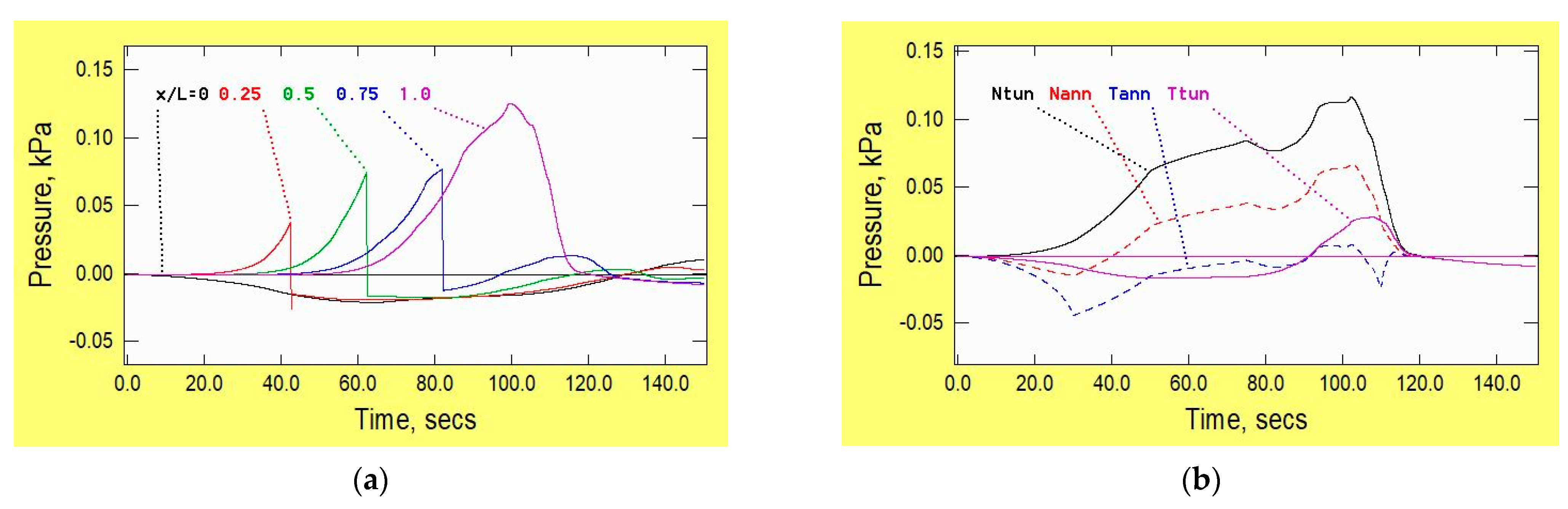
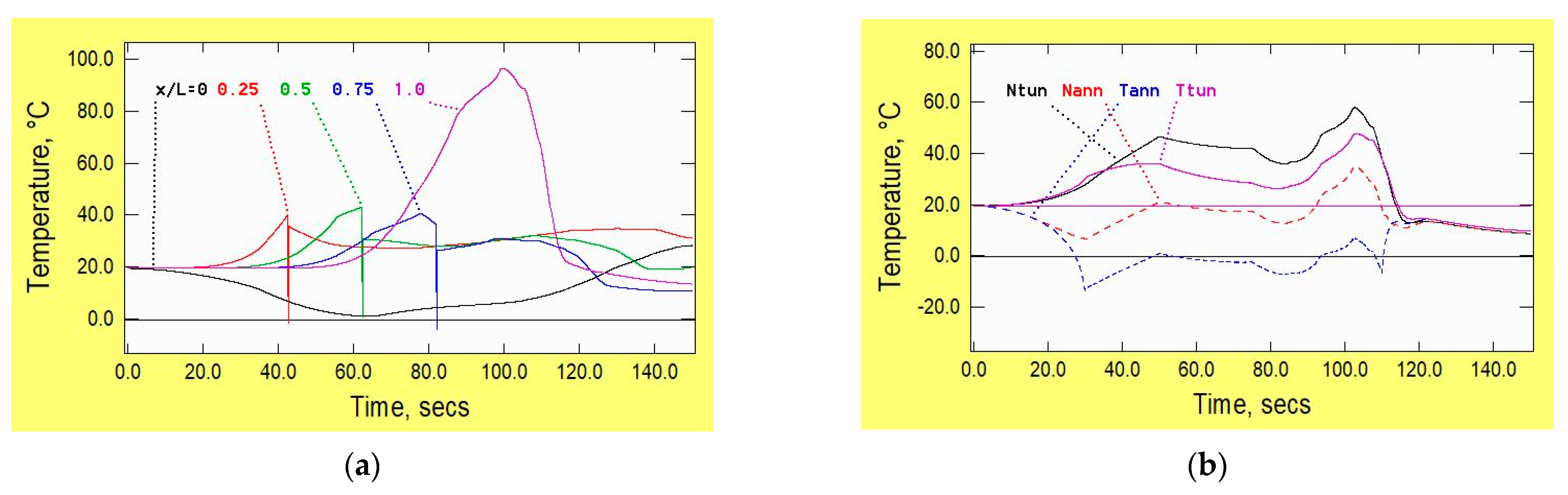

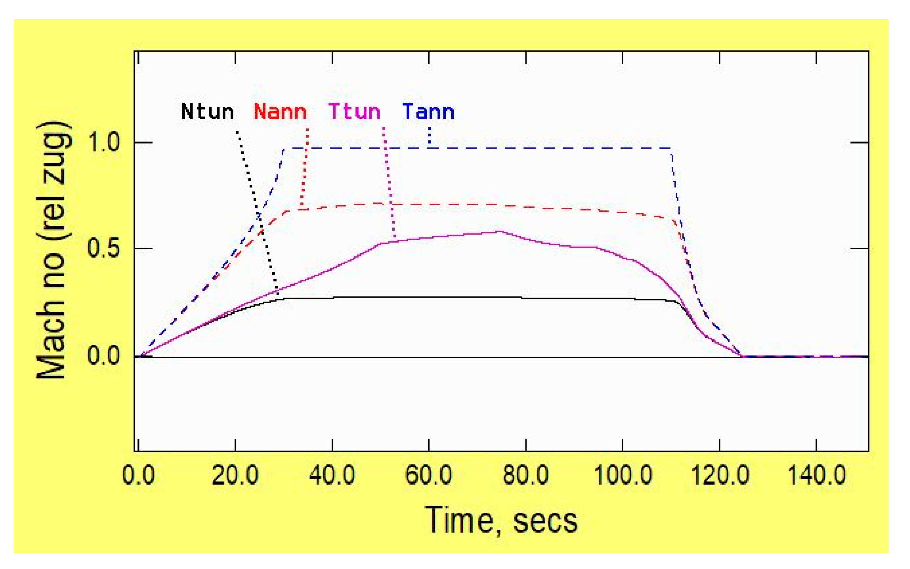
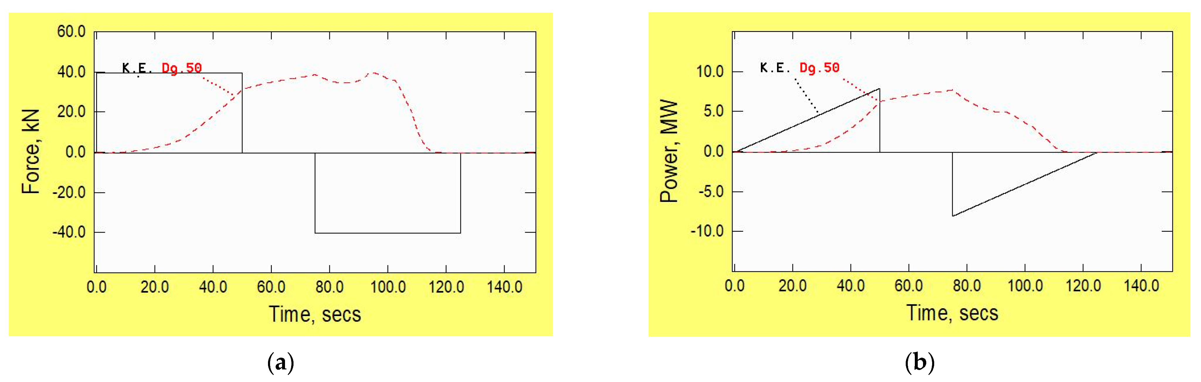
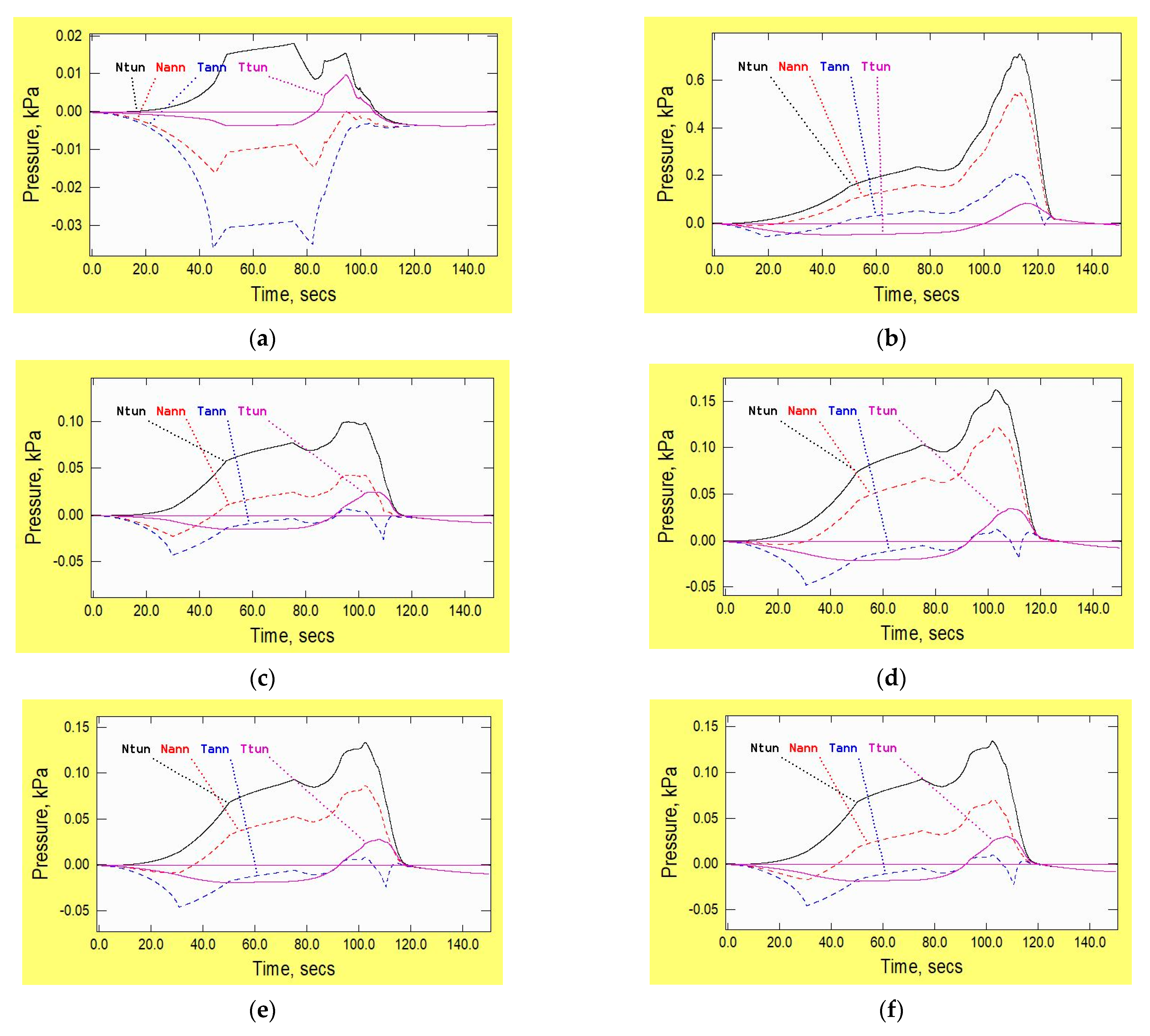
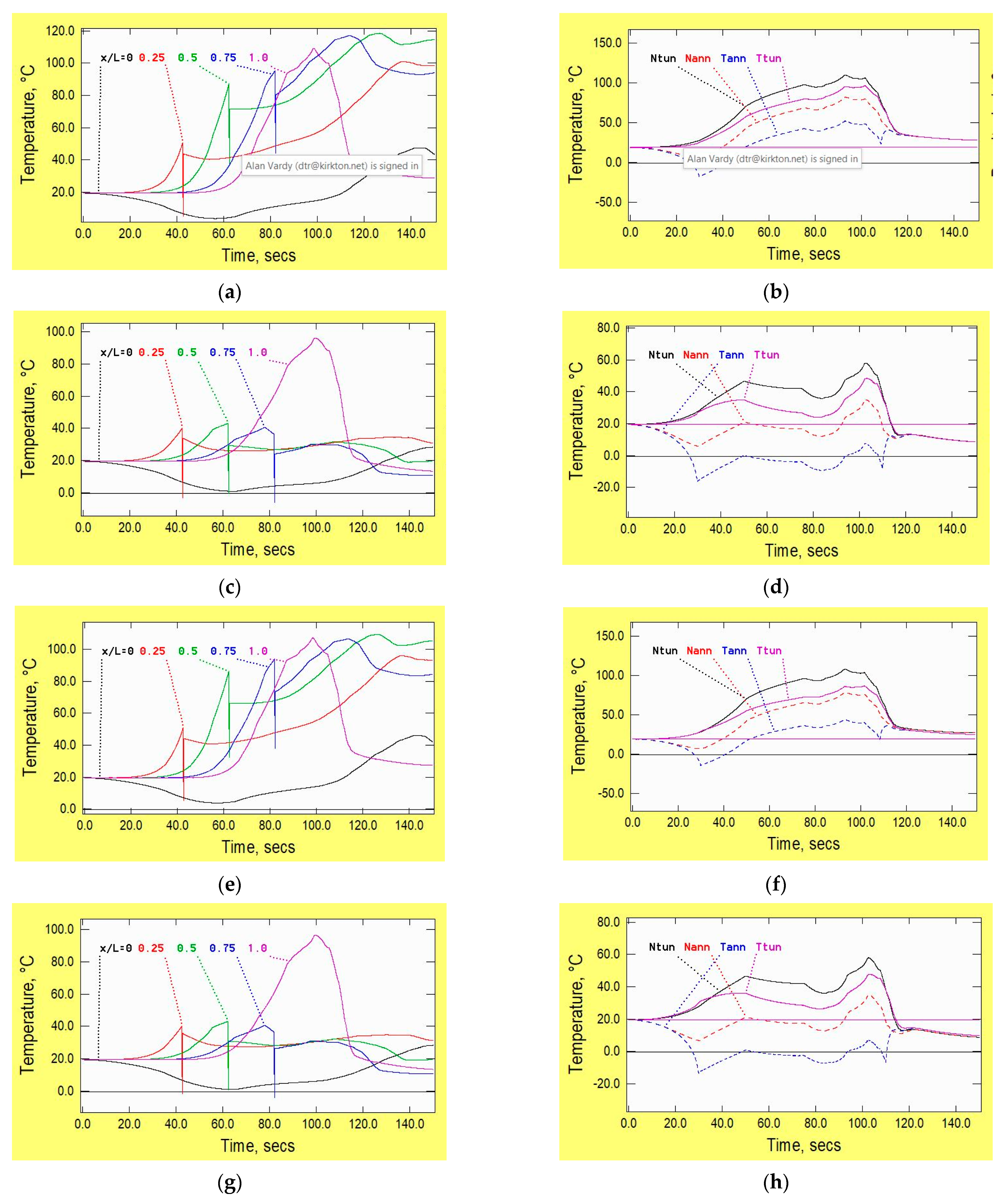
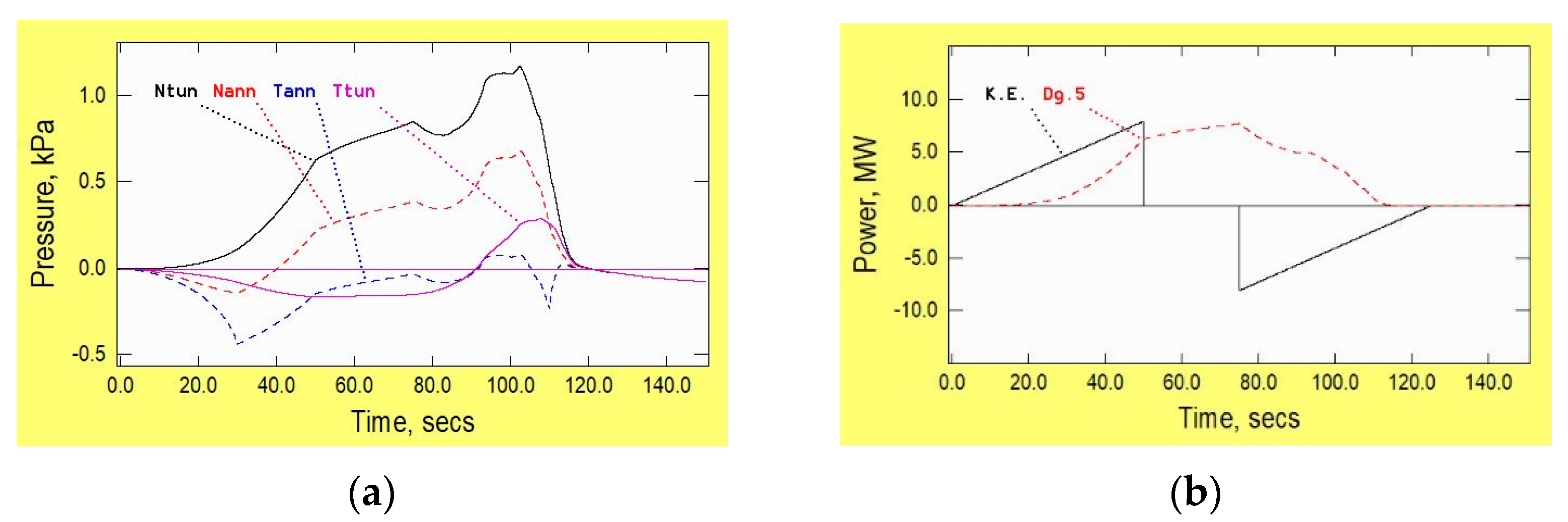

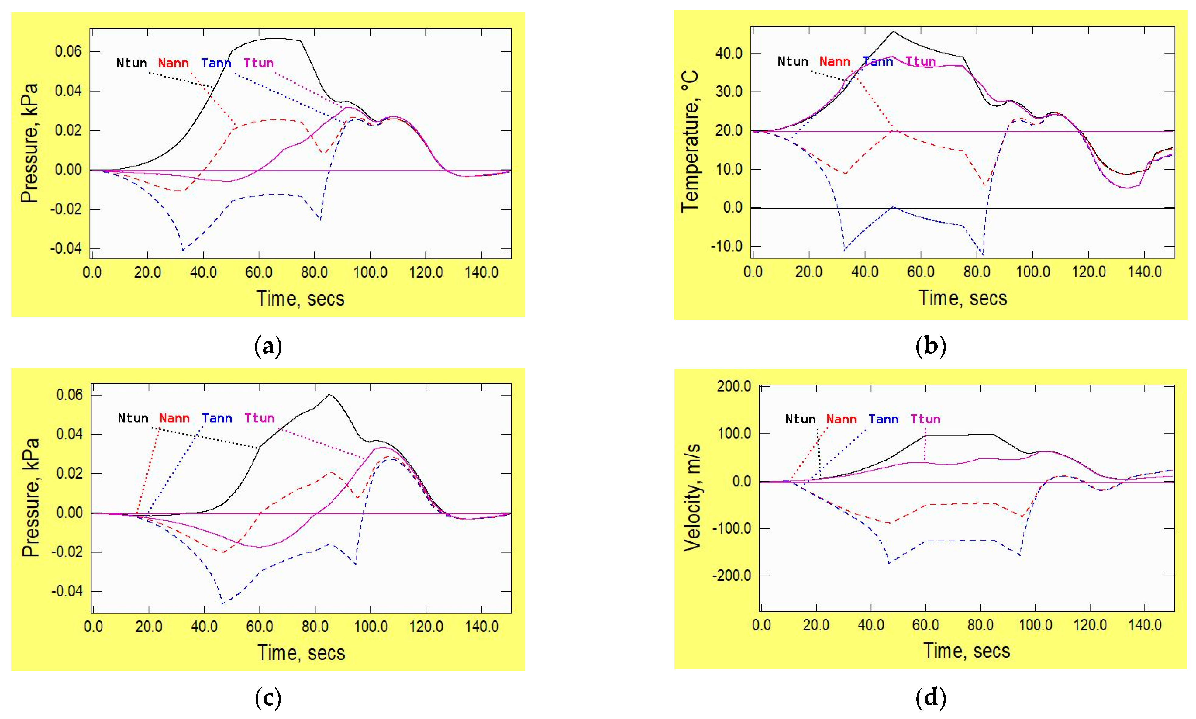

Disclaimer/Publisher’s Note: The statements, opinions and data contained in all publications are solely those of the individual author(s) and contributor(s) and not of MDPI and/or the editor(s). MDPI and/or the editor(s) disclaim responsibility for any injury to people or property resulting from any ideas, methods, instructions or products referred to in the content. |
© 2023 by the author. Licensee MDPI, Basel, Switzerland. This article is an open access article distributed under the terms and conditions of the Creative Commons Attribution (CC BY) license (https://creativecommons.org/licenses/by/4.0/).