Developing a Generalized Regression Forecasting Network for the Prediction of Human Body Dimensions

Abstract

With the increasing demand for intelligent custom clothing, the development of highly accurate human body dimension prediction tools using artificial neural network technology has become essential to ensuring high-quality, fashionable, and personalized clothing. Although support vector regression (SVR) networks have demonstrated state-of-the-art (SOTA) performances, they still fall short on prediction accuracy and computation efficiency. We propose a novel generalized regression forecasting network (GRFN) that incorporates kernel ridge regression (KRR) within a multi-strategy multi-subswarm particle swarm optimizer (MMPSO)-SVR nonlinear regression model that applies a residual correction prediction mechanism to enhance prediction accuracy for body dimensions. Importantly, the predictions are generated using only a few basic body size parameters from small-batch samples. The KRR regression model is employed for preliminary residual sequence prediction, and the MMPSO component optimizes the SVR parameters to ensure superior correction of nonlinear relations and noise data, thereby yielding more accurate residual correction value predictions. The GRFN hybrid model is superior to SOTA SVR models and increases the root mean square performance by 91.73–97.12% with a remarkably low mean square error of 0.0054 ± 0.07. This outstanding advancement sets the stage for marketable intelligent apparel design tools for the fast fashion industry.

1. Introduction

With the many recent improvements in global living standards, human clothing requirements now prioritize diversity and personalization with small-batch, made-to-measure fashion solutions. As such, body dimension and posture measurement prediction supported by artificial neural networks (ANNs) has become a crucial human–machine engineering field. From these tools, new computer-aided ergonomic garment design tools can be paired with three-dimensional (3D) non-contact body scanning and virtual fitting techniques that avoid the use of various calipers, tape measures, and Martin-style anthropometric measuring tools [1]. These anthropometric methods utilize stature percentiles for body segments, which can lead to large errors in practice. Hence, the fashion industry demands more cost-effective, accurate, and efficient non-percentile anthropometric methods that cater to clothing and human-centered product designs [2].

In recent years, research on predicting human body dimensions and shapes using artificial intelligence technologies has been widely conducted, mainly including various prediction methods such as multiple linear regression (MLR) [3,4,5], back-propagation (BP) ANN [6,7,8,9], radial basis function (RBF) ANN [2,10,11], and support vector regression (SVR) methods [12,13,14]. Su et al. [3] used an MLR model that incorporates easily measurable features, including the thickness/width parameters of cross-sections, with the objective of constructing additional lower-body characteristics. Galada and Baytar [4] used the U.S. size database to train a new lasso regression method that establishes relationships between key predictor variables related to crotch length to improve the fit of bifurcated garments. Chan et al. [5] utilized 3D anthropometric data to forecast the relevant parameters in shirt pattern design by deploying an ANN with a linear regression model to reveal the relationship between patterns and body measurements. However, the nonlinearity in the relationships between different body parts becomes more pronounced, and the MLR model struggles to accurately capture this characteristic. Liu et al. [6] provided a back-propagation (BP) ANN that uses anthropometric data to predict human body dimensions, providing robust support for custom clothing. Furthermore, Liu et al. [7] introduced digital clothing pressure from virtual try-ons as input parameters and employed a BPNN model to predict the fit of clothing, including tight, well-fitted, or loose. This research has expanded the potential applications of BPNN methods in the field of clothing design. However, due to the random selection of initial weights and thresholds in BPNN, the network may become stuck in local minima, thereby diminishing its fitting performance. To overcome this challenge, Cheng et al. [8] employed a genetic algorithm to implement a GA-BP-K-means model to cluster data and enhance body shape prediction. This method involves using a genetic algorithm to optimize the initial parameters of the BPNN. Similarly, Cheng et al. [9] addressed the issue of predicting underwear pressure using an improved GA algorithm combined with a BPNN model. The improved GA algorithm accelerated the BP neural network’s convergence speed and enhanced underwear pressure prediction accuracy. In addition to BPNN, other ANN models, such as the radial basis function neural network (RBF-NN) are also often used to estimate body sizes. For example, Liu et al. [10] trained a model on clothing knowledge to extract key human body feature parameters using factor analysis with a combined RBF-NN and linear regression method. This enabled the prediction of detailed human body dimensions with a small number of feature parameters. Wang et al. [11] employed an RBF-NN to estimate complex parameters to improve the comfort and adaptability needed for sportswear. The generalized regression neural network, of Wang et al. [2], utilizes a particular RBF-NN, and demonstrated a high degree of accuracy in predicting 76 specific human body parameters, without the need for manual measurements or 3D body scanning. This model has shown remarkable predictive capabilities, in line with the growing trend of predicting human body dimensions rather than relying on direct measurements.

Support vector regression (SVR) networks comprise state-of-the-art (SOTA) ANN models, but they still fall short in prediction accuracy and computation efficiency. However, SVR models are the most suitable for nonlinear regression problems in which only small-batch samples are available, and they are robust to outliers. Li and Jing [12] used an SVR network to construct a regression model for two-dimensional width and depth features and the corresponding circumference sizes of three important measurement parts (i.e., bust, waist, and hip) of young female samples. However, the establishment of this method relied on cross-sectional data of the human body and cannot avoid the need for 3D scanning. Rativa et al. [13] demonstrated the possibility of superior performance over traditional linear regression methods by employing an SVR model with a Gaussian kernel for the estimation of height and weight using anthropometric data alone. While the results of this method were said to be insensitive to race and gender, in practical application, there may be other unaccounted factors that challenge the model’s robustness. Li et al. [14] introduced a data-driven model based on particle swarm optimization (PSO) to optimize the least-squares support vector machine (LSSVM) algorithm. This model was applied to solve the problems of garment style recognition and size prediction for pattern making. Tailoring experience was used as the training basis to improve prediction accuracy. However, the ambiguity of the relationship between the variables made the aforementioned single direct prediction model unsuitable for the fashion industry, due to the diversity of body shapes and precise body dimensions. Although the prediction results exhibit a certain level of accuracy, there is ample room for improvement.

Furthermore, anthropometry found extensive applications in the field of intelligent clothing design. For instance, Wang et al. [15] employed fuzzy logic and genetic algorithms to generate initial clothing patterns. They utilized SVR to learn about the quantitative relationships between clothing structural lines, control points, and pattern parameters. These relationships were then used to predict and adjust the pattern parameters, achieving pattern adaptability. Liu et al. [16] proposed a machine learning framework that combines hybrid feature selection and a Bayesian search to estimate missing 3D body measurements, addressing the challenge of incomplete data in 3D body scanning. The study found that this approach leverages hybrid feature selection and the Bayesian search to enhance the performance of random forest (RF) and XGBoost 0.72, particularly in filling in missing data, where RF outperforms XGBoost. Wang et al. [17] introduced an approach that utilizes multiple machine learning frameworks, including RBF-NN, GA, PNN (probabilistic neural network), and SVR, for interactive personalized clothing design. This method enhanced the capability of personalized clothing design by estimating body dimensions, generating customized design solutions, quantifying consumer preferences, predicting clothing fit, and self-adjusting design parameters.

The global optimization of parameters can improve prediction accuracy and generalizability, and modernized meta-heuristic swarm intelligence optimization algorithms can simulate individual and group behaviors that are suitable for complex optimization problems. They also rapidly converge with fewer parameters, and are easily implemented [18]. However, multimodal swarm intelligence algorithms cannot conquer optimization problems caused by global exploration and local exploitation imbalances that deprive late iterations of their required data diversity [19]. The literature provides a wealth of PSO improvements related to this via parameter weight adjustments (e.g., linear decay [20], chaotic dynamism [21], and S-shaped decay [22]), population topologies (e.g., static neighborhood [23], dynamic neighborhood [24], and hierarchical structure particle subswarms [25]), and evolutionary learning strategies (e.g., comprehensive learning strategy [26], generalized opposition-based learning strategy [27], orthogonal learning strategy [28], and dimensional learning strategy [29]). As stated by the no-free-lunch theorem [30], the identification of a singular method that can be universally regarded as superior to all others for every task is not feasible. However, owing to discrepancies between the two aspects of global exploration and local exploitation, multi-swarm techniques can be used to maintain the population diversity needed to facilitate information flows within subpopulations. Hence, heterogeneous multi-subpopulation techniques have become effective in enhancing PSO algorithms [31].

In this study, we propose a novel generalized regression forecasting network (GRFN), that combines kernel ridge regression (KRR) prediction with a new multi-strategy, multi-subswarm PSO (MMPSO)-SVR model to considerably reduce large errors in human body dimension prediction. The resulting highly accurate small-batch, data-driven human body dimension prediction scheme does not require stature percentile anthropometric measurements and 3D body reconstruction. Our hybrid model only needs a few basic body size parameters to obtain detailed body dimensions. For our experiment, we used the processes of Liu et al. [6] to collect lower-body data from 106 women and applied principal factor analysis so that the KRR-based regression model can establish a multi-variate nonlinear correlation map of parameters. This generates preliminary prediction results as a residual sequence that can be used to fit the data linearly. To deal with nonlinear and noisy data, our model takes the residual of the predicted KRR output as input. A residual correction prediction mechanism is employed to improve the fit and predictive performance of our hybrid model, addressing the following aspects: improving prediction accuracy, accounting for unmodeled factors and making adjustments, correcting model bias, and enhancing model robustness. For further optimization, we apply teaching and co-optimization to the MMPSO algorithm, which divides the population into three role-based subgroups: teachers, students, and independent learners. The ability of the MMPSO model to search for the global optimum primarily depends on the diversity of the population. The SVR then balances exploration and exploitation using a diversity-focused multi-strategy search to avoid local optima. Finally, the estimated values of the predicted body parameters are obtained by combining the KRR results with the corrected MMPSO-SVR residuals. Thus, our hybrid model provides verifiable human body dimension predictions that can work with small-batch samples.

In summary, this study makes the following contributions:

(1)

Our GRFN utilizes a novel KRR-based MMPSO-SVR nonlinear regression network to achieve residual correction prediction. The proposed hybrid model applies a direct approach that utilizes a few basic body measurements to predict other, more detailed human body dimensions from small-batch samples. The results clearly validate the proposed model, as it outperforms state-of-the-art (SOTA) SVR models in terms of both prediction accuracy and reliability.

(2)

Our MMPSO model adopts a teaching–learning co-optimization scheme in which a teacher subgroup performs enhanced self-learning searching and a student subgroup constructs learning exemplars under the guidance of the teacher group via sub-swarm. The independent subgroup performs self-perceptive search behaviors, and the MMPSO algorithm enhances population diversity while preventing subswarms from becoming trapped in local optima. Competitive results are achieved in terms of optimization convergence and stability in terms of most classical benchmarks.

(3)

Our GRFN network utilizes just a few basic body size parameters as input and obtains detailed human body dimensions and establishes correlations between key body size parameters and clothing pattern sample sizes. This model eliminates the need for anthropometric measurements and 3D body reconstructions, making it more accurate and easily implemented than existing regression models. Consequently, it offers a novel and efficient solution for clothing and human-centered product design.

The rest of this paper is arranged as follows: In Section 2, the research methods are elaborated. Section 3 further describes the GRFN model design alongside the MMPSO algorithm. The effective performance of the proposed hybrid KRR-based MMPSO-SVR model is then reported in Section 4, and a discussion and conclusions for the paper are presented in Section 5, along with directions for future research.

2. Research Methods

2.1. KRR

The KRR regression model employs a kernel function to nonlinearly transform the original sample data and map it to a high-dimensional space [32,33]. By weighting the regularization terms and the $L_2$ norm with these parameters, the model effectively prevents overfitting and enhances its generalizability. For the training set, ${\left\{\left(x_i,y_i\right)\right\}}_{i=1}^n$, $x_i\in {ℝ}^p$, and $y_i\in ℝ$ are the i-th observation and response variables, respectively. The count of observations is denoted as $n$, whereas the count of independent variables is denoted as $p$. The loss function is expressed as follows:

$$\underset{f\in \mathcal{H}}{f=\arg \min }\left\{\frac{1}{n}{\displaystyle \sum _{i=1}^n{‖f(x_i)-y_i‖}_2^2+\lambda {‖f‖}_{\mathcal{H}}^2}\right\},\lambda >0,$$

(1)

$$f(x_i)={\displaystyle {\sum }_{j=1}^n{\widehat{\alpha }}_j}\kappa (x_j,x_i),$$

(2)

where ${‖\cdot ‖}_{\mathcal{H}}^2$ is the $L_2$ norm form in the function space, $\lambda$ is the regularization parameter, and $\kappa (\cdot ,\cdot )$ is the kernel function. Given an $n\times n$ kernel matrix, $K_N$, the KRR estimate is given as follows:

$$\widehat{\alpha }={\left(K_N+\lambda nI\right)}^{-1}y,$$

(3)

$$\widehat{y}={\displaystyle {\sum }_{i=1}^n{\widehat{\alpha }}_i}\kappa (x_j,x_i),$$

(4)

where $x$ represents the provided sample, and $\widehat{y}$ stands for the predicted value. We use cross-validation to calculate the minimum value of the Bayesian information criterion (BIC) for the training set to select the best model’s $\lambda$ value.

2.2. PSO

Particles can be divided into whole or nearest neighbor types, which can be further divided into global and local versions (i.e., GPSO and LPSO, respectively). The GPSO [20] algorithm takes the position and velocity, ${\mathrm{X}}_i={(x_{i1},x_{i2},\dots ,x_{id})}_{i=1}^N$ and ${\mathrm{V}}_i={(v_{i1},v_{i2},\dots ,v_{id})}_{i=1}^N$, respectively. In this context, variable $D$ denotes the number of dimensions, $d\in \left[1,2,\dots ,D\right]$, the search zone consists of a population size of $N$, and the formulas for updating velocity and position are implemented as follows:

$$v_{id}^{(t+1)}=w{v}_{id}^{(t)}+c_1{r}_1(p{b}_{id}^{(t)}-x_{id}^{(t)})+c_2{r}_2(p{b}_{gb,d}^{(t)}-x_{id}^{(t)}),$$

(5)

$$x_{id}^{(t+1)}=x_{id}^{(t)}+v_{id}^{(t)},$$

(6)

where $v_{id}^{}$ represents the velocity of the particle located at i-th index in the d-th dimension, and t and t + 1 represent the iteration numbers of the previous and current rounds, respectively. Symbol $w$ denotes the inertial weight associated with the memory part of the particle, $c_1$ represents the cognitive acceleration factor, while $c_2$ corresponds to the social acceleration factor. Given matrix $r_1,r_2\in {[0,1]}^D$, $p{b}_i=[p{b}_{i1},p{b}_{i2},\dots ,p{b}_{iD}]$ signifies the historical best position of particle $p_i$, and $p{b}_{gb}=[p{b}_{g{b}_1},p{b}_{g{b}_2},\dots ,p{b}_{g{b}_D}]$ represents the optimal position of the entire population. If the dimensional bounds of $\left|v_{id}\right|$ exceed the maximum velocity, ${\mathrm{V}}_{\max }$, then $v_{id}=\mathrm{sgn}(v_{id}){\mathrm{V}}_{\max }$.

For LPSO, speed $v_{id}$ is updated as shown in Equation (7), where the historically best position of the nearest-neighbor particle is $p_{sb}=[p_{s{b}_1},p_{s{b}_2},\dots ,p_{s{b}_D}]$:

$$v_{id}^{(t+1)}=w{v}_{id}^{(t)}+c_1{r}_1(p{b}_{id}^{(t)}-x_{id}^{(t)})+c_2{r}_2(p_{sb,d}^{(t)}-x_{id}^{(t)}).$$

(7)

2.3. SVR

An SVM uses few-shot learning to support structural risk minimization and solve classification and regression problems [34]. An SVM can be divided into classification and regression operations, where SVR is widely used to handle few-shot and nonlinear regression problems. Within a provided training set, $S=\left\{{\left.\left(x_i,y_i\right)\right|}_{i=1}^N\right\}$, $x_i\in ℝ$ denotes the input vector, and $y_i\in ℝ$ is the corresponding output. The SVR builds an optimally separated hyper-plane in a high-dimensional (sometimes infinite) feature space, maximizing the margin among the nearest training data points. Symbol $\phi (x_i)$ represents the eigenvector of $x_i$ within the decision function, and empirical risk can be calculated using the $\epsilon$-insensitive loss function. A regularization term is used to enhance the optimization of structural risk and achieve comprehensive regression:

$${\mathcal{L}}_{\epsilon }=\max (0,\left|y_i-{\mathit{w}}^T\cdot \phi (x_i)-b\right|-\epsilon ).$$

(8)

When sample data are found in the $\epsilon$-insensitive interval band, its loss is zero. Variables ${\xi }_i$ and ${\xi }_i^{\ast }$ are considered slack variables in this context. Specifically, ${\xi }_i$ is used to represent the training error exceeding a certain threshold of $+\epsilon$, whereas ${\xi }_i^{\ast }$ is used to represent a training error below a threshold of $-\epsilon$. Finding hyper-planes $\mathit{w}$ and $b$ are convex quadratic programming problems.

$$\underset{\omega ,b,\xi ,{\xi }^{*}}{\min }\frac{1}{2}{‖\mathit{w}‖}^2+C{\displaystyle \sum _{i=1}^m({\xi }_i}+{\xi }_i^{*}),$$

(9)

$$s.t.\left\{\begin{array}{l}{\mathit{w}}^T\cdot \phi (x_i)+b-y_i\le \epsilon +{\xi }_i\hfill \\ y_i-{\mathit{w}}^T\cdot \phi (x_i)-b\le \epsilon +{\xi }_i^{*}\hfill \\ {\xi }_i,{\xi }_i^{*}\ge 0,i=1,2,\dots ,m\hfill \end{array}\right.,$$

(10)

where $\epsilon$ denotes the maximum deviation, and C is the trade-off factor of model complexity and error. By incorporating Lagrange multipliers ${\alpha }_i$ and ${\alpha }_i^{\ast }$, the optimization problem of Equations (9) and (10) is transformed into a dual optimization problem, and an optimal hyper-plane regression decision function is obtained using the KKT condition.

$$\left\{\begin{array}{l}f(x)={\displaystyle {\sum }_{i=1}^m({\alpha }_i^{\ast }-{\alpha }_i)\cdot \kappa (x_i,x)}+b^{\ast }\hfill \\ \kappa (x_i,x_j)=\exp \left(-\frac{{‖x_i-x_j‖}^2}{2\sigma }\right)=\exp (-g{‖x_i-x_j‖}^2)\hfill \end{array}\right.,$$

(11)

where $\kappa (\cdot ,\cdot )$ is the Gaussian kernel function, and $g$ stands for the kernel coefficient.

3. Methodology of the GRFN

3.1. General Scheme

The architecture of the generalized regression forecasting network (GRFN) is visualized in Figure 1. To improve accuracy and efficiency, we establish a non-linear correlation between easily measured body parameters and other detailed dimensions that are normally difficult to integrate for customized clothing design. First, we extract the principal factors by preprocessing Liu et al.’s human body dimension dataset consisting of the data of 106 young women [6]. To prepare the model, the anthropometric dataset is preprocessed, and normalized for input to the KRR regression model. An appropriate $\lambda$ value is selected by 10-fold cross-validation, multivariate regression is constructed, and the residual sequence between predicted and ground-truth data is calculated. These residual and measured sequences are input to the SVR model, where rough $C$ and $g$ hyperparameters are obtained using the grid search method, and the best pair $(C_{best},g_{best})$ are obtained using the MMPSO-SVR model. The KRR-based regression estimations are combined with predicted residual correction values to obtain the dimensional parameters of the human body. Finally, detailed body dimensions are obtained by using a few basic body size parameters input to our GRFN model. An interactive intelligent pattern-making system is employed to generate 2D patterns, and garments are simulated on a virtual 3D avatar for clothing display.

3.2. Hybrid Prediction Process

The hybrid prediction process is illustrated in Figure 2. The details are more concisely elaborated in the following subsections.

3.2.1. Step 1: Data PreProcessing

The data are subjected to min-max normalization, resulting in a range of $[0,1]$:

$$x_i^{\prime }=\frac{x_i-x_{\min }}{x_{\max }-x_{\min }},$$

(12)

where variable $x_i$ denotes the original data, and $x_i^{\prime }$ represents the normalized data, whose sequences are bounded by location boundaries of $x_{\max }$ and $x_{\min }$. Then, the length and perimeter factors with large contribution rates (i.e., height, waist circumference, hip circumference, waist circumference height, and hip circumference height) are used as key feature inputs, and randomly assigned to the training and testing sets.

3.2.2. Step 2: KRR Regression Modeling

The minimum BIC value is calculated from the training data to select the best $\lambda$ value [35]. The ridge regression model is then used to obtain the predicted ${\widehat{y}}_i^{\prime }$ value of the training sequence data, and the residual value is provided:

$$e_i=y_i-{\widehat{y}}_i^{\prime },$$

(13)

where the i-th residual value is represented by $e_i$, and $y_i$ corresponds to measured value. The residual sequence data pair $\{(y_i,e_i)\}$ is then constructed as input to the MMPSO-SVR residual prediction model.

3.2.3. Step 3: Calculation of the SVR Kernel Function

The parameters of the SVR kernel function are estimated to obtain approximate values. Subsequently, the fitness function is then defined as follows:

$$fit(e_i)=\sqrt{\frac{1}{n}{\displaystyle {\sum }_{i=1}^n{({\widehat{e}}_i-e_i)}^2}},$$

(14)

where $n$ is the quantity of samples, and ${\widehat{e}}_i$ is the predicted residual values after applying the grid search method on the i-th sample. The grid search method searches a large range that is enlarged and reduced twice to obtain the optimized penalty factor and RBF kernel function parameter pair $(C,g)$.

3.2.4. Step 4: MMPSO-SVR Residual Correction

Population position and velocity are initialized, where population is divided into three subgroups, each representing a feasible solution hyperparameter pair $(C,g)$. In the search zone, the fitness function of each particle is computed to ascertain its individual extreme value, represented as $pb$, and its group extreme value, represented as $p{b}_{gb}$. The MMPSO co-optimization algorithm uses teaching and learning to find $p{b}_{gb}$ and locate the global optimum. The termination condition is iteratively determined, and 10-fold cross-validation is utilized to determine the optimal combination of SVR kernel function parameters, $\{(y_i,e_i)\}$, as input. Variable $e_i$ represents the supervisory information used for training, which gives us the residual prediction value, ${\widehat{e}}_i$.

3.2.5. Step 5: Residual Correction Combination Prediction

By combining ${\widehat{y}}_i^{\prime }$ and ${\widehat{e}}_i$, the estimated body size parameter is obtained:

$${\widehat{y}}_i={\widehat{y}}_i^{\prime }+{\widehat{e}}_i.$$

(15)

Thus, body dimensions for pattern making can be predicted with an accuracy sufficient for garment production.

3.3. Construction of MMPSO Algorithm for Body Dimension Prediction

3.3.1. Sine Chaotic Opposite-Based Learning Population Initializations

Initial population diversity is crucial to improving the search zone, optimization precision, and convergence speed. The chaotic parameters are characterized by their randomness, ergodicity, and regularity. Currently, the most common chaotic mappings [36] include tent, logistic, and sine types. Sine chaos is a self-mapping mode characterized by infinite folding. During optimization, opposite-based learning (OBL) can quickly find an approximate reverse solution. Accordingly, an elitist greedy strategy is adopted to select the optimal population, effectively improving the quality of solutions in the search zone. Therefore, sine chaos is employed to generate an initial population with the greatest diversity. The one-dimensional mapping of the sine chaos is expressed as follows:

$$\left\{\begin{array}{l}{Z}_{i+1}=\sin (2/Z_i),i=0,1,\dots ,N\hfill \\ -1\le Z_i\le 1,Z_i\ne 0\hfill \end{array}\right..$$

(16)

To avoid the generation of fixed and zero points in the closed interval $[-1,1]$, the initial value should not be set to zero. The sine chaos sequence is converted into a set of $D$ pseudo-random numbers, $Z_{i,j}$, and is inversely mapped into variables $x_{i,j}$:

$$x_{i,j}=l{b}_j+(u{b}_j-l{b}_j)\cdot abs(z_{i,j}),$$

(17)

where $[l{b}_j,u{b}_j]$ is the dynamic search zone boundary along dimension j, and $z_{i,j}$ represents the j-th dimensional component of the i-th pseudo-random number. Next, the OBL strategy [27] is utilized to generate an opposite-based population, ${\mathrm{X}}^{\prime }=\{{\mathrm{X}}_i^{\prime },i=1,2,\dots ,N\}$, and the individual term, $x_{i,j}^{\prime }$, can be defined as

$$x_{i,j}^{\prime }=k\cdot (l{b}_j+u{b}_j)-x_{i,j},$$

(18)

where the generalized coefficient, denoted as $k\in \mathrm{U}(0,1)$, is sampled from a uniform distribution. Finally, employing the elitist greedy strategy, the reversed population, ${\mathrm{X}}^{\prime }$, and initial population after sine-mapping, $\mathrm{X}$, are merged into a new population, ${\mathrm{X}}_{new}=\{{\mathrm{X}}^{\prime }\cup \mathrm{X}\}$. From this, the initial $N$ particles with the most suitable fitness score are chosen as $\mathrm{X}$. In an initialization learning environment, the heterogeneous search behavior of multi-subpopulation diversities is utilized. According to a fitness value difference, $D_f$, ascending sort, the population particles are grouped into elite (i.e., teacher subgroup ${\mathrm{X}}_{ST}$), ordinary (i.e., independent learner subgroup ${\mathrm{X}}_{SI}$), and poor (i.e., student subgroup ${\mathrm{X}}_{SS}$) categories. The classification method is as follows:

$${\mathrm{X}}_i\in \left\{\begin{array}{l}\begin{array}{l}{\mathrm{X}}_{ST}, if D_f\le {\lambda }_r\hfill \\ {\mathrm{X}}_{SI}, if {\lambda }_r\le D_f\le (1-{\lambda }_r)\hfill \end{array}\hfill \\ {\mathrm{X}}_{SS}, if D_f\ge (1-{\lambda }_r)\hfill \end{array}\right.,$$

(19)

where swarm ratio ${\lambda }_r=30\%$, and $1-{\lambda }_r=70\%$.

3.3.2. Teaching and Learning Co-Optimization Strategy

Inspired by the literature [31], the teaching and learning co-optimization strategy for the teacher and student subpopulations includes two stages: global and local tuning. With global tuning, the teacher subpopulation uses a ring-topological comprehensive learning strategy to search based on self-cognition and social learning behaviors to obtain information from neighbors, enhance search efficiency and stability, and accelerate convergence. Social learning consists of group induction guidance and ring neighborhood particle learning:

$$v_{id}^{(t+1)}=w_1{v}_{id}^{(t)}+c_1{r}_1(p{b}_{fi(d)}^{(t)}-x_{id}^{(t)})+c_2{r}_2{\beta }^{ST}(p{b}_{gb,d}^{(t)}-x_{id}^{(t)})+c_3{r}_3(r{b}_{id}^{(t)}-x_{id}^{(t)}),$$

(20)

where the linear decreasing inertia weight is expressed as $w_1:0.9~0.4$, and the first acceleration factor is $c_1:2.5~2.0$, which is linearly decreasing. The second acceleration factor is $c_2:0.5~2.0$, which is linearly increasing, and the third acceleration factor is $c_3:2.0~0.0$, which is linearly decreasing. Function $f_i(d)=[f_i(1),f_i(2),\dots ,f_i(D)]$ represents $pb$ of the i-th particle and must conform to requirements in the d-th dimension, $r{b}_i=[r{b}_{i1},r{b}_{i2},\dots ,r{b}_{iD}]$ is the i-th particle’s closest neighbor in the ring topology, and ${\beta }^{ST}=0.5$ is the social learning tendency coefficient. These items are used to improve the performance of particles and enhance their self-search. To strike a balance between exploring and exploiting particles across different dimensions, the CLS is used to define the individual learning probability, $pc$, of each particle, which generates a $[0,1]$-interval random number for each dimension. A random number performs better than learning probability in solving the multipeak function. CLS adopts an aging strategy to regenerate the historical optimal solution, $p{b}_{fi(d)}$, of individual nearest neighbors when the number of stagnant neighbors exceeds the threshold of seven. During global tuning, a subgroup stagnation state-checking mechanism is employed to detect whether the subpopulations of teachers and students are stagnant. Then, the fitness deviation of the optimal solution is calculated for generations t and t − 1 subgroups to judge whether any are stagnant.

$$\delta sbest(t+1)=fit(p{b}_{sb}^{(t+1)})-fit(p{b}_{sb}^{(t)})\le 0,$$

(21)

where the fitness function is $fit(\cdot )$, and $p{b}_{sb}$ represents the locally optimal solution within the subgroup. When $\delta sbest(t+1)<0$, the capacity for global search of the subgroup is normal, and the stagnant state counter, $Sta{g}_s$, is zero. When $\delta sbest(t+1)=0$, the capacity for global search of the subpopulation weakens and $Sta{g}_s=Sta{g}_s+1$. If $Sta{g}_s\ge C_{t1}$, where $C_{t1}$ is the stagnation threshold [37] selected as $T_{\max }/10$, where $T_{\max }$ denotes the fixed number of iterations, the subgroup is identified as having entered stagnation. Then, the local tuning operation is employed to reinvigorate the search capability and counteract stagnation.

During local tuning, particle disturbance update and refresh compensation operations are used. Inspired by the literature [38], during the particle disturbance update, a search operator guided by the historical extremum of the induction group is used to remove bias from the search and improve population diversity as follows:

$$\mathrm{new}{\mathrm{X}}_i={\mathrm{X}}_i+{\zeta }_1({\mathrm{X}}_i-{\mathrm{X}}_k)+{\zeta }_2(p{b}_{gb}-{\mathrm{X}}_i),$$

(22)

where ${\zeta }_1$, ${\zeta }_2$ are random numbers in the range of $[-1,1]$ and $[0,1.5]$, respectively. $k$ is a random index in $[1,N]$, and $k\ne i$. The new search operator guides particle-balanced exploration and exploitation by inducing historical extrema in the group. During the particle disturbance update operation, an individual particle adopts an optimal greedy strategy. Thus, if the new position’s fitness value, ${\mathrm{X}}_i^{(t+1)}$, surpasses the initial fitness value, ${\mathrm{X}}_i^{(t)}$ is activated with ${\mathrm{X}}_i^{(t+1)}$, and the state counter is activated as $Sta{g}_i=0$; otherwise, the particles will not be activated, and $Sta{g}_i=Sta{g}_i+1$ is performed. If $Sta{g}_i>C_{t2}$, where $C_{t2}$ is $0.8(D\times N)/2$ after many iterations, the position of the new particles may still not meet the requirements of optimization. Hence, the subgroup is vulnerable to the potential of converging towards a local optimum. Therefore, a refresh compensation operation is used to reverse the subgroup stagnation and improve quality. Two particle historical extrema are used for an arithmetic crossover operation to generate the new position:

$$\mathrm{new}{\mathrm{X}}_i^{\prime }={\mathrm{X}}_i+{\vartheta }_1(p{b}_{k1}-p{b}_{k2}),$$

(23)

where ${\vartheta }_1$ is a random number in $[-1,1]$, $k_1,k_2\in [1,N_1]$ is a random number, and $p{b}_{k1}$ and $p{b}_{k2}$ are individual historical optima of the randomly selected particles, $k_1$ and $k_2$, respectively. The refresh compensation operation performs a random search and shares individual historical extrema. The advantages of individual candidate solutions are related to the selected particle vector, ${\mathrm{X}}_i^{(t)}$, and the difference vector, $p{b}_{k1}-p{b}_{k2}$, which are chemotaxis operations. During the early progress of our algorithm, the step size of the difference vector is usually larger than it will be later, which is beneficial for initially expanding the search zone. The vector then reduces over time to improve the local development ability. Generally, the step size of the difference vector is continuously adjusted to accommodate various stages and attain superior optimization.

To enhance the search efficiency of the student group, its particles are generally initially far from the optimal area and must be studied under the guidance of the teacher subgroup. During global tuning, the student subgroup employs a search behavior based on social self-cognition; its velocity update equations are as follows:

$$v_{id}^{(t+1)}={\omega }_1{v}_{id}^{(t)}+c_1{r}_1{\beta }_i^{CT}(p{b}_{id}^{(t)}-x_{id}^{(t)})+c_2{r}_2{\beta }_i^{ST}(p{b}_{gb,d}^{(t)}-x_{id}^{(t)}),$$

(24)

$${\beta }_i^{CT}=\left\{\begin{array}{l}1, \mathrm{if} {\alpha }_i>0.5\hfill \\ 0, \mathrm{otherwise}\hfill \end{array}\right.,$$

(25)

$${\beta }_i^{ST}=\left\{\begin{array}{l}1, \mathrm{if} {\beta }_i^{CT}>0.5\hfill \\ 0, \mathrm{otherwise}\hfill \end{array}\right.,$$

(26)

where ${\beta }_{}^{CT}$ is the self-cognition tendency coefficient, ${\beta }_{}^{ST}$ is the social learning tendency coefficient, and variable ${\alpha }_i~\mathrm{U}(0,1)$ represents a random number that is drawn from a uniform distribution over the closed interval $[0,1]$. The student subgroup adopts two-stage tuning to enhance its local optimization ability, with which both the teacher and student subgroups can fully exploit their advantages and jointly promote the exploitation and convergence accuracy of the large algorithm. Simultaneously, to hasten student subgroup convergence, the students generate new learning examples under the guidance of the teacher, and they are sorted based on the fitness function [39]. If the fitness value of a student, $y_j$, surpasses that of the teacher group, $x_i$, the velocity update of $y_j$ is distributed and updated around its original position. The velocity calculation formula for the student subgroup particles following the instruction is as follows:

$$v_{jd}^{(t+1)}=w_c{v}_{jd}^{(t)}+{\gamma }_2(x_{id}-y_{jd})\cdot \exp (-\mu \cdot dis(x_i,y_j)),$$

(27)

$$dis(x_i,y_j)={\displaystyle {\sum }_{d=1}^D{(x_{id}-y_{jd})}^T}(x_{id}-y_{jd}),$$

(28)

where $w_c=0.8$ is the adjustment coefficient, symbol $x_i$ denotes the spatial position of the i-th individual within the teacher subgroup, whereas symbol $y_j$ denotes the spatial position of the j-th individual within the student subgroup, and the function $dis(x_i,y_j)$ represents the Euclidean distance between particles $x_i$ and $y_j$, where ${\gamma }_2=1.2$ and $\mu =2.0$.

3.3.3. Multi-Swarm Dynamic Regroup Strategy

The independent learner group employs a dynamic regrouping strategy for multiple subswarms to generate learning exemplars. First, the dynamic regroup learning strategy of multiple subswarms is used to maintain population diversity. In each iteration, the velocity of particles i within each dynamic subgroup is updated using Equations (29) and (30) to enhance the global exploration performance:

$$v_{id}^{(t+1)}=w_2{v}_{id}^{(t)}+c_4{r}_4(p{b}_{id}^{(t)}-x_{id}^{(t)})+c_5{r}_5{\beta }_i^{ST}(p{b}_{sb,d}^{(t)}-x_{id}^{(t)}),$$

(29)

$${\beta }_i^{ST}=\left\{\begin{array}{l}1, \mathrm{if} {\alpha }_i>0.5\hfill \\ 0, \mathrm{otherwise}\hfill \end{array}\right.,$$

(30)

where ${\omega }_2$ is a self-adjusting inertial weight that controls the search range and improves the global search capability. $c_4$, $c_5$ are constants of 1.49445, and ${\beta }_i^{ST}$ represents the coefficient of the social learning tendency of the independent learner group subpopulation as perceived by particle $p_i$. When ${\alpha }_i>0.5$, ${\beta }_i^{ST}=1$ represents the social cognitive ability perceived by $p_i$; otherwise, there is no social ability. Simultaneously, a nonuniform Gaussian mutation operator is applied as an update perturbation to augment the subpopulation’s global search performance of the independent learner group during early iterations and improve the local exploitation ability in later iterations.

$${\tilde{\mathrm{X}}}_{id}^{(t)}=\left\{\begin{array}{l}{\mathrm{X}}_{id}^{(t)}+\mathrm{\Delta }(t,N((u{b}_d-{\mathrm{X}}_{id}^{(t)}),{\sigma }^2(t)), \mathrm{rand} < 0.5\hfill \\ {\mathrm{X}}_{id}^{(t)}-\mathrm{\Delta }(t,N(({\mathrm{X}}_{id}^{(t)}-l{b}_d),{\sigma }^2(t)), \mathrm{rand}\ge 0.5\hfill \end{array}\right.,$$

(31)

$$\mathrm{\Delta }(t,y)=y\cdot (1-{\mathrm{rand}}^{{(1-t/T_{\max })}^2}),$$

(32)

$${\sigma }^2(t)={\sigma }_0^2\cdot \exp (-(t/T_{\max })),$$

(33)

where $\mathrm{\Delta }(t,y)$ adaptively adjust the step length. ${\sigma }_0^2$ is the initial variance and the symbol ${\sigma }^2(t)$ denotes the particle’s mutation amplitude in the t-th iteration.

3.3.4. Refined Search Strategy for the Global Optimal Solution

The teacher, independent learner, and student group subpopulations exchange information among subpopulations based on the global optimal solution, $p{b}_{gb}$, to improve performance and convergence. When the number of stagnant updates for $p{b}_{gb}$ surpasses the predefined threshold, $m=5$, a fine search is implemented based on the t-distribution mutation and reverse learning using a beetle antennae search (BAS) [40]. In the refined search phase, if a globally optimal particle becomes trapped in a local optimum, we employ the opposite learning method to obtain a reverse solution, thus broadening the search range of the globally optimal particle. This OBL strategy is integrated into the MMPSO algorithm; its mathematical description is as follows:

$$p{b^{\prime }}_{{}_{gb}}^{(t)}=ub+r_6(lb-p{b}_{{}_{gb}}^{(t)}),$$

(34)

$$p{b}_{{}_{gb}}^{(t+1)}=p{b^{\prime }}_{{}_{gb}}^{(t)}+b_1(p{b}_{{}_{gb}}^{(t)}-p{b^{\prime }}_{{}_{gb}}^{(t)}),$$

(35)

where $p{b^{\prime }}_{{}_{gb}}^{(t)}$ represents the reverse of the global optimum solution at iteration t, and the global optimal solution of the t + 1 iteration is denoted as $p{b}_{{}_{gb}}^{(t+1)}$. Items $ub$ and $lb$ represent the spatial boundaries of the search region, $r_6$ denotes a random number that follows a uniformly distributed random number within interval $\left[0,1\right]$, and $b_1$ denotes the coefficient for controlling information exchange [41], which is mathematically expressed by the following formula:

$$b_1={\left(\frac{T_{\max }-t}{T_{\max }}\right)}^t.$$

(36)

The t-distribution is a continuous probability distribution that amalgamates features from both Gaussian and Cauchy distributions. A degree-of-freedom parameter governs its behavior, enabling a balance between global and local searches. This parameter enables the shape of the distribution to be adjusted so that larger values have higher peaks, such as a Gaussian shape, which has improved local search capability. Smaller values result in flatter shapes, such as those of the Cauchy distribution, which results in the improvement of global development capabilities. During the fine search, the global optimal solution is further optimized by introducing a t-distribution mutation operator. The mathematical expression is as follows:

$$p{b}_{gb,d}^{(t+1)}=p{b}_{gb,d}^{(t)}+\eta \cdot \mathrm{dir}\cdot (x_{\max ,d}-x_{\min ,d})\cdot TD(t),$$

(37)

$$\mathrm{dir}=\mathrm{rands}(1,D),\mathrm{dir}=\mathrm{dir}/\mathrm{norm}(\mathrm{dir}),$$

(38)

where $p{b}_{gb,d}^{}$ represents the global optimal solution for the d-th dimension, the region within the d-dimensional search zone is $[x_{\min ,d},x_{\max ,d}]$, $\eta$ represents the particle rotation direction with a value of +1/−1, symbol $\mathrm{dir}$ is the normalized direction vector, and $TD(t)$ is the degree of freedom of the t-distribution mutation operator. Like the BAS method, which simulates a beetle using its two antennae to sense the direction of the most intense food smell and thereby decide whether to move left or right, the current globally optimal particle determines its distance to the optimal solution based on its left or right orientation. The particle rotation direction, $\eta$, is calculated in the following manner:

$$\left\{\begin{array}{l}p{b}_{gb}^{left}(t)=p{b}_{gb}^{}(t)+d_r(t)\cdot \mathrm{dir}/2\hfill \\ p{b}_{gb}^{right}(t)=p{b}_{gb}^{}(t)-d_r(t)\cdot \mathrm{dir}/2\hfill \end{array}\right.,$$

(39)

$$d_r(0)=step, d_r(t+1)=d_r(t)\times 0.95,$$

(40)

$$\eta =\mathrm{sgn}(fit(p{b}_{gb}^{right})-fit(p{b}_{gb}^{left})),$$

(41)

where $p{b}_{gb}^{left}(t)$ denotes the t-th iteration’s global optimum after the search process in the left direction, $p{b}_{gb}^{right}(t)$ denotes the t-th iteration’s global optimum after the search process in the right direction, $d_r(t)$ represents the sensing range diameter of the t-th iteration’s global optimal particle, the initial value assigned to variable “step” is 10, and function $\mathrm{sgn}(\cdot )$ denotes the sign function used to determine the direction of the individual’s next search.

By integrating the t-distribution mutation strategy with the BAS algorithm and the OBL strategy, the perturbation of the global optimal solution updates; these steps are alternately executed based on the calculated selection probability, $\mathrm{Pr}$.

$$\mathrm{Pr}=-\exp {\left(1-\frac{t}{T_{\max }}\right)}^{20}+0.05.$$

(42)

If $\mathrm{rand}<\mathrm{Pr}$, the OBL strategy is employed to introduce disturbances into the update process of the global optimal solution; otherwise, the process of choosing the t-distribution mutation strategy is employed, which incorporates the BAS, to update the target position. Additionally, an elitist greed-based approach is employed to determine whether the target position should be updated.

3.3.5. The Full Process of the MMPSO

Based on the improvements discussed in Section 3.3.1, Section 3.3.2, Section 3.3.3 and Section 3.3.4, the full MMPSO process is described with Algorithm 1.

Algorithm 1: The full MMPSO process

Input: $\mathrm{Swarm} \mathrm{size} N, \mathrm{inertial} \mathrm{weights} w_1$$, w_2$$, w_c$$, \mathrm{Swarm} \mathrm{ratio} {\lambda }_r$$, \mathrm{acceleration} \mathrm{factor} c_1,c_2,c_3$$, \mathrm{maximum} \mathrm{iterations} T_{\max }$$, Const=0.15$$, m=5$$, \mathrm{location} \mathrm{boundary} [x_{\min }^d,x_{\max }^d]$$, \mathrm{velocity} \mathrm{boundary} [v_{\min }^d,v_{\max }^d]$$, \mathrm{and} d=1,2,\dots ,D$;

Output: $\mathrm{Global} \mathrm{optimal} \mathrm{solution} p{b}_{gb}$;

Initialize initial position $x_i^d$ and velocity $v_i^d$ of particles; Compute the fitness value of each particle $p_i$; while $t=1,2,\dots ,T_{\max }$ do   if $Sta{g}_s\le C_{t1}$ then     for  $i\leftarrow 1:N_1$ do  /* teacher subgroup global tuning */       Update ${\mathrm{X}}_{ST}$ subgroup ${\mathrm{V}}_i$ and ${\mathrm{X}}_i$ using Equations (6) and (20);     end for     Check ${\mathrm{X}}_{ST}$ subgroup stagnation using Equation (21);   else  /* teacher subgroup local tuning */      ${\mathrm{X}}_i$ perform particle disturbance update operation using Equation (22);      if $Sta{g}_i>C_{t2}$ then        ${\mathrm{X}}_i$ perform refresh compensation operation using Equation (23);      end if   end if   if $fit({\mathrm{X}}_i)>fit\_avg$ then     $w_2=w_2(t)+Const;$ if $w_2>0.99$, $w_2=0.99$ end;   else     $w_2=w_2(t)-Const;$ if $w_2<0.2$, $w_2=0.2$ end;   end if   for $i\leftarrow 1:N_2$ do  /* independent learner subgroup */     Update $\mathrm{the} \mathrm{velocity} \mathrm{of} {\mathrm{X}}_{SI}$ subgroup using Equations (29) and (30);     ${\mathrm{X}}_i$ perform nonuniform Gaussian mutation using Equations (31)–(33);   end for   if $Sta{g}_s\le C_{t1}$ then     for$i\leftarrow 1:N_3$ do   /* student subgroup global tuning */       Update ${\mathrm{X}}_{SS}$ subgroup ${\mathrm{V}}_i$ and ${\mathrm{X}}_i$ using Equations (6) and (24);     end for     Check for ${\mathrm{X}}_{SS}$ subgroup stagnation using Equation (21);   else   /* student subgroup local tuning */     ${\mathrm{X}}_i$ perform particle disturbance update operation using Equation (22);     if $Sta{g}_i>C_{t2}$ then       ${\mathrm{X}}_i$ perform refresh compensation operation using Equation (23);     end if   end if   Update particle of student subgroup using Equations (27) and (28);   Calculate all particles $p{b}_i$ and $p{b}_{gb}$ of the population;   if $\mathrm{rand}<\mathrm{Pr}$ then     Update $p{b}_{gb}$ with OBL strategy using Equations (34) and (35);   else     Update $p{b}_{gb}$ with t-distribution mutation using Equations (37)–(41);   end if   Update ${\mathrm{X}}_{ST}$ subgroup with aging strategy the CLPSO-like algorithm;   Update ${\mathrm{X}}_{SI}$  subgroup with multi-swarm dynamic regrouping strategy; end while return $p{b}_{gb}$, $gbestval$;

3.3.6. Time Computational Complexity Analysis

MMPSO’s time complexity is analyzed according to Algorithm 1. In MMPSO, we assume that the parameters are initialized, where the swarm size of the input is denoted as N, the spatial dimension is denoted by D, and the fixed number of iterations is indicated as T. The time computational complexity formula for the basic PSO is $\mathcal{O}(T\cdot N\cdot D)$. In MMPSO, we assume that the time complexity needed to initialize the population phase of the parameter is $\mathcal{O}(N\cdot D)$. During global tuning, we determine whether the stagnant state counter, $Sta{g}_s$, is greater than threshold $C_{t1}$ and activate state detector $Sta{g}_i>C_{t2}$. Then, the particle disturbance update and refresh compensation operations in the local tuning phase are performed, and the time computational complexity of the worst-case scenario is represented as $\mathcal{O}(2N_1)$. The independent learner subgroups alternately execute dynamic multi-swarm reorganization learning strategies, and their time computational complexity is $\mathcal{O}(N_2\cdot D)$. The student subgroup learns under the supervision of the teacher subgroup, and the global tuning phase performs a self-cognitive or social cognitive search. The local tuning phase then performs a particle disturbance update and refreshes the compensation operations. In the event of the most unfavorable circumstances, the time computational complexity becomes $\mathcal{O}(N_3\cdot D+2N_3)$. During the fine-search phase of the global optimal solution, the time computational complexity associated with the selection of the dimensional vector for updating the global optimal solution is $\mathcal{O}(D)$. Consequently, when the stopping criterion for the MMPSO algorithm is characterized by a fixed number of Iterations, denoted as $T$, the total time computational complexity of the MMPSO algorithm can be expressed as $\mathcal{O}(T\cdot N\cdot D)$.

4. Experimental Results and Discussion

Within this section, model human body dimensions were evaluated using two experiments to assess model performance. Experiment 1 entailed the classical CEC2005 test suite for MMPSO task validation, and Experiment 2 validated the model’s human body size prediction based on real-world small-batch samples. All experiments were implemented on a 64-bit operating system, a Core i7-6500U CPU with a main frequency of 2.5 GHz, 16-GB memory, and a MATLAB 2018b programming/runtime environment.

4.1. Experimental Setup

4.1.1. Description of Experimental Data

Following Ref. [6], Liu et al. utilized the Vitus Smart 3D body scanning device to create a dataset comprising measurements from 106 female undergraduate students, never pregnant, aged 20 to 25 years, in the northeastern region of China. The participants’ heights ranged from 151.5 to 173.2 cm, and their weights ranged from 40 to 71 kg based on intermediate sizes provided by the Chinese National Standard, GB/T 1335.2-2008: [42] Standard Sizing Systems for Garments–Women. Prior to commencement of this study, we addressed ethical compliance issues and made relevant disclosures. Notably, all participants provided informed consent, allowing their measurement data to be obtained using a 3D body scanner in an automated manner. The final measurement dataset exclusively provided our measurement testing data, and we completely anonymized the data items. Hence, no personally identifiable participant information was retained. Furthermore, our reference few-shot anthropometric database is publicly available, as explained in appendix 1 in reference [43]. To this end, we utilized this open-source anthropometric database to validate the efficacy of our hybrid model.

Table 1. Descriptive statistics on dimension measurements.

Measurements	Abbr.	Min	Max	Mean	Median	SM	SD	CV (%)
Stature	ST	151.5	173.2	161.9	160.9	161.4	5.21	3.22
Waist Height	WH	93.4	111.0	101.2	100.5	100.8	3.97	3.92
Abdomen Height	AH	86.2	103.3	94.5	94.1	94.2	3.80	4.02
Hip Height	HH	75.2	91.1	82.9	82.4	82.7	3.76	4.54
Crotch Height	CH	64.8	80.7	71.7	71.2	71.5	3.29	4.59
Knee Height	KH	39.0	48.1	43.5	43.3	43.3	2.04	4.70
Waist Height	WH	58.3	81.3	69.1	68.8	69.0	4.94	7.14
Hip Circumference	HC	78.0	101.8	92.2	92.5	92.4	4.75	5.15
Thigh Circumference	TC	42.4	60.8	52.9	52.6	52.7	3.75	7.09
Knee Circumference	KC	31.6	43.9	37.4	37.3	37.3	2.26	6.05
Abdomen Circumference	AC	65.0	91.2	79.2	79.2	79.2	5.35	6.75
Total Crotch Length	TCL	64.5	93.9	73.2	72.8	73.1	4.10	5.61
Crotch Width	CW	17.2	22.2	19.7	19.8	19.7	1.04	5.28

Notes: Measurements are in centimeters (cm). Height (ST), waist circumference (WC), hip circumference (HC), crotch height (CH), waist height (WH), abdominal height (AH), hip height (HH), knee height (KH), total crotch length (TCL), thigh circumference (TC), abdomen circumference (AC), knee circumference (KC), and crotch width (CW). The sum mean (SM) is the average of the sums of the upper quartile, lower quartile, and overall mean. Standard deviation (SD) and the coefficient of variation (CV) are also listed.

displays the descriptive statistics of the body dimensions and relevant measures, such as mean, median, and central tendency.

4.1.2. Factor Analysis

We used maximum orthogonal factor analysis variance to extract two principal factors from 13 observation items and eliminate multicollinearity among variables. The rotated component matrix is represented in

Table 2. Rotated component matrix.

No.	Measurements	Abbr.	Component 1	Component 2
1	Stature	ST	0.970	0.209
2	Waist Height	WH	0.964	0.215
3	Abdomen Height	AH	0.958	0.223
4	Hip Height	HH	0.960	0.198
5	Crotch Height	CH	0.890	−0.021
6	Knee Height	KH	0.909	0.273
7	Waist Circumference	WC	0.047	0.915
8	Hip Circumference	HC	0.258	0.918
9	Thigh Circumference	TC	0.163	0.927
10	Knee Circumference	KC	0.232	0.794
11	Abdomen Circumference	AC	0.220	0.920
12	Total Crotch Length	TCL	0.445	0.553
13	Crotch Width	CW	0.045	0.852

, which lists the scores of each sample and factor. Based on the total variance explanation provided in

Table 3. Sum of squares of rotated loadings.

Component	Factor	Eigenvalues	% of Variance	Cumulative %
Factor 1	Height Factor	5.725	44.040	44.040
Factor 2	Circumference Factor	5.302	40.787	84.827

, the height factor and perimeter (circumference) coefficient were found to represent most of the information on lower body size.

To avoid large prediction errors caused by large differences in input data, both easy- and difficult-to-measure key human body parameters were normalized. To mitigate interference resulting from varying body shapes, the dataset was divided into distinct training and testing sets, with divisions based on variables, such as stature and waist girth. The training set underwent cross-verification k times to evaluate the results.

4.1.3. Performance Metrics

To quantitatively compare the predictive accuracies of the models, this study employed the root mean square error ($e_{RMSE}$), mean absolute error ($e_{MAE}$), and coefficient of determination ($R^2$). The corresponding equations are presented as follows:

$$e_{RMSE}({\mathrm{Y}}_{obs},{\mathrm{Y}}_{pred})=\sqrt{\frac{1}{n}{\displaystyle \sum _{i=1}^n{(y_i-{\widehat{y}}_i)}^2}},$$

(43)

$$e_{MAE}({\mathrm{Y}}_{obs},{\mathrm{Y}}_{pred})=\frac{1}{n}{\displaystyle \sum _{i=1}^n\left|y_i-{\widehat{y}}_i\right|},$$

(44)

$$R^2({\mathrm{Y}}_{obs},{\mathrm{Y}}_{pred})=1-{{\displaystyle {\sum }_{i=1}^n{(y_i-{\widehat{y}}_i)}^2/{\displaystyle {\sum }_{i=1}^n(y_i-\overline{\widehat{y}})}}}^2,$$

(45)

where $y_i$ and ${\widehat{y}}_i$ represent observed and predicted values, respectively, and the variable $\overline{\widehat{y}}$ denotes the average of the predicted values derived from a collection of $n$ samples.

4.2. Comparison of PSO Variant Algorithms for Benchmark Functions

4.2.1. Benchmark Functions and Parameter Settings for PSO Variants

To evaluate the optimization performance of the proposed MMPSO, the classical CEC 2005 test suite [44] was selected as the experimental benchmark. The test set consisted of four types of functions: F01–F05 (unimodal (UN)), F06–F12 (multimodal (MN)), F10 and F11 (rotation), F13 and F14 (expanded (EF)), and F15–F25 (hybrid composition (CF)). The test suite can comprehensively and objectively reflect the optimization performance of an algorithm. For a more comprehensive evaluation and analysis, we compared the MMPSO algorithm with seven well-known PSO variants: HIDMSPSO, HCLPSO, HCLDMSPSO, CLPSO, DMSPOS, EPSO, and FDRPSO. The PSO variants’ parameter settings were established as indicated in

Table 4. Parameters settings for PSO variants.

Algorithms	Year	Parameter Settings	Reference
FDRPSO	2003	$w:0.9\sim 0.4,c_1=c_2=1.0,c=2.0$	Peram et al. [45]
DMSPSO	2005	$w=0.729,c_1=c_2=1.49445$	Liang et al. [24]
CLPSO	2006	$w:0.9\sim 0.4,c_1=c_2=1.49445,m=7$	Liang et al. [26]
HCLPSO	2015	$w:0.99\sim 0.2,c_1:2.5\sim 0.5,c_2:0.5\sim 2.5$	Lynn et al. [46]
EPSO	2017	$w:0.9\sim 0.4,c_1=c_2=2.0$	Lynn et al. [47]
HCLDMSPSO	2020	$w_1:0.99\sim 0.29,w_2,c_1:2.5\sim 0.5,c_2:0.5\sim 2.5,P_m=0.1$	Wang et al. [48]
HIDMSPSO	2020	$w_1:0.99\sim 0.2,w_2,c_1:2.5\sim 0.5,c_2:0.5\sim 2.5$	Varna et al. [49]
MMPSO	–	$w_1:0.9\sim 0.4,w_2:0.99\sim 0.2,w_c=0.8,c_1:2.5\sim 0.5,$ $c_2:0.5\sim 2.5,c_3:2.0\sim 0,c_4=c_5=1.49445$	–

.

4.2.2. Numerical Experimental Results

The performance of the MMPSO and several well-known PSO variants was evaluated using a benchmark test suite. Following the acquisition of the results from 30 independent runs of each algorithm, the evaluation metrics were determined based on the average value (mean) and standard deviation (Std) of each benchmark function. The mean reflects the overall trend of convergence and optimization ability, whereas the Std indicates the stability of the algorithm and its capacity to evade local optima.

The dimensions needed to solve the problem were 30, the upper limit for the total number of fitness evaluations was 300,000, the population size was set to 40, and the sizes of the three heterogeneous subgroups (i.e., teacher, independent learner, and student) were 12, 16, and 12, respectively. The MMPSO algorithm in F04, F06, F08, F10, F11, F14, F17–F20, and F22–F25 benchmark functions were compared with the alternative PSO variants, revealing clearly improved solution accuracy, as demonstrated in

Table 5. Solution accuracy of benchmark functions (30-dim).

Function	MMPSO (Ours)		HIDMSPSO		HCLPSO		CLPSO
	Mean	Std	Mean	Std	Mean	Std	Mean	Std
F01	5.11 × 10−14	1.79 × 10−14	7.96 × 10−14	3.11 × 10−14	8.43 × 10−14	2.87 × 10−14	5.49 × 10−14	1.13 × 10−14
F02	2.96 × 10−12	4.59 × 10−12	1.79 × 10−10	1.31 × 10−10	8.23 × 10−5	1.10 × 10−4	1.09 × 103	2.81 × 102
F03	3.97 × 105	2.24 × 105	4.77 × 105	2.38 × 105	9.41 × 105	5.40 × 105	1.28 × 107	4.05 × 106
F04	21.98	24.53	67.49	54.41	6.65 × 102	3.40 × 102	8.59 × 103	1.85 × 103
F05	2.12 × 103	4.98 × 102	5.89 × 102	4.69 × 102	3.28 × 103	6.14 × 102	4.41 × 103	3.99 × 102
F06	0.42	1.25	64.56	51.18	2.48	2.06	1.04	1.64
F07	9.61 × 10−3	8.87 × 10−3	1.33 × 10−2	1.50 × 10−2	1.91 × 10−2	1.51 × 10−2	0.75	0.12
F08	20.52	6.99 × 10−2	20.61	0.12	20.80	6.70 × 10−2	20.89	7.08 × 10−2
F09	18.39	7.43	40.62	9.34	1.10 × 10−13	3.30 × 10−14	5.68 × 10−14	0
F10	27.95	5.65	45.79	14.15	56.19	14.22	1.13 × 102	16.75
F11	8.48	2.65	15.89	5.18	20.69	2.94	24.57	1.64
F12	8.16 × 103	4.38 × 103	6.61 × 103	6.99 × 103	4.78 × 103	4.57 × 103	1.35 × 104	4.09 × 103
F13	1.95	0.27	3.68	0.98	1.48	0.22	1.82	0.19
F14	11.09	0.50	11.74	0.49	12.36	0.88	12.64	0.21
F15	3.44 × 102	1.38 × 102	3.66 × 102	84.25	89.39	87.76	37.57	20.42
F16	96.69	40.84	1.51 × 102	1.66 × 102	1.08 × 102	37.83	1.57 × 102	22.33
F17	1.13 × 102	1.06 × 102	1.16 × 102	1.02 × 102	1.28 × 102	49.22	2.31 × 102	33.91
F18	8.88 × 102	16.82	9.05 × 102	3.32	8.96 × 102	43.79	9.10 × 102	20.59
F19	8.81 × 102	12.52	9.04 × 102	0.49	9.10 × 102	20.95	9.15 × 102	1.32
F20	8.66 × 102	30.63	9.05 × 102	0.67	8.98 × 102	39.44	9.13 × 102	20.61
F21	5.00 × 102	2.27 × 10−12	5.00 × 102	2.88 × 10−13	4.99 × 102	3.62	5.00 × 102	3.51 × 10−13
F22	7.51 × 102	48.62	8.38 × 102	20.67	9.06 × 102	16.39	9.75 × 102	15.37
F23	5.34 × 102	1.77 × 10−4	5.34 × 102	4.28 × 10−4	5.34 × 102	4.03 × 10−4	5.34 × 102	3.16 × 10−4
F24	2.00 × 102	1.12 × 10−13	2.00 × 102	1.54 × 10−12	2.00 × 102	1.62 × 10−12	2.00 × 102	3.09 × 10−12
F25	2.00 × 102	2.13 × 10−13	2.00 × 102	1.36 × 10−12	2.00 × 102	1.56 × 10−12	2.00 × 102	4.46 × 10−10
Function	DMSPSO		EPSO		FDRPSO		HCLDMSPSO
	mean	Std	mean	Std	mean	Std	mean	Std
F01	1.89 × 10−15	1.13 × 10−14	5.49 × 10−14	1.03 × 10−14	1.15 × 10−13	3.49 × 10−14	5.87 × 10−14	1.03 × 10−14
F02	21.54	13.82	8.90 × 10−13	2.88 × 10−13	2.24 × 10−11	6.33 × 10−11	3.00 × 10−2	3.56 × 10−2
F03	5.89 × 106	2.59 × 106	3.23 × 105	1.41 × 105	3.75 × 105	1.75 × 105	1.13 × 106	3.95 × 105
F04	1.33 × 103	5.42 × 102	1.11 × 102	1.13 × 102	3.10 × 102	1.71 × 102	43.79	45.38
F05	2.43 × 103	5.03 × 102	4.26 × 103	8.31 × 102	3.45 × 103	6.82 × 102	2.29 × 103	3.70 × 102
F06	52.31	38.36	1.33	1.56	9.29	22.72	26.64	21.56
F07	1.74 × 10−2	1.11 × 10−2	2.20 × 10−02	2.11 × 10−2	1.51 × 10−2	1.25 × 10−2	6.66 × 10−3	9.80 × 10−3
F08	20.53	4.64 × 10−2	20.89	8.25 × 10−2	20.87	7.81 × 10−2	20.68	0.12
F09	13.77	10.22	0.33	0.65	30.89	7.94	29.71	5.28
F10	55.15	6.94	57.71	14.98	59.22	14.85	28.55	5.99
F11	28.84	1.45	23.06	3.39	19.23	4.71	10.34	3.54
F12	6.80 × 103	5.47 × 103	4.87 × 103	4.45 × 103	7.05 × 103	8.83 × 103	3.97 × 103	3.70 × 103
F13	3.93	0.51	2.20	0.40	3.00	0.68	2.59	0.52
F14	12.48	0.27	11.83	0.62	11.89	0.67	11.09	0.64
F15	3.55 × 102	83.72	1.09 × 102	97.06	3.13 × 102	1.13 × 102	3.23 × 102	78.42
F16	2.62 × 102	1.95 × 102	1.14 × 102	51.86	2.46 × 102	1.87 × 102	63.18	36.36
F17	1.78 × 102	1.26 × 102	1.34 × 102	76.35	2.95 × 102	1.99 × 102	1.23 × 102	1.38 × 102
F18	9.09 × 102	1.74	9.01 × 102	46.79	9.16 × 102	4.10	8.91 × 102	41.82
F19	9.08 × 102	2.43	9.00 × 102	45.62	9.16 × 102	4.33	8.88 × 102	44.98
F20	9.08 × 102	2.41	9.11 × 102	30.62	9.16 × 102	4.09	9.06 × 102	20.21
F21	5.00 × 102	2.48 × 10−13	4.97 × 102	14.30	5.80 × 102	1.63 × 102	5.00 × 102	1.85 × 10−13
F22	9.09 × 102	12.10	9.23 × 102	20.78	9.26 × 102	16.80	9.05 × 102	10.41
F23	5.34 × 102	2.38 × 10−4	5.34 × 102	4.15 × 10−4	6.70 × 102	2.19 × 102	5.34 × 102	1.89 × 10−4
F24	2.00 × 102	7.97 × 10−13	2.00 × 102	1.39 × 10−12	2.00 × 102	1.46 × 10−12	2.00 × 102	1.32 × 10−13
F25	2.00 × 102	5.77 × 10−13	2.00 × 102	8.09 × 10−13	2.00 × 102	1.10 × 10−12	2.00 × 102	2.95 × 10−13

Notes: Values in bold font indicate the optimal results.

. Figure 3A illustrates how the MMPSO algorithm demonstrated excellent performance in terms of finding the global optimum using unimodal functions. Furthermore, the MMPSO algorithm performed well when solving multimodal functions and expanded functions, as illustrated in Figure 3B. In terms of algorithm stability, the standard deviations of the F04, F05, F06–F08, F10, F17–F18, and F23–F25 benchmark functions exhibited superior performance over the alternative PSO variants. The final ranking algorithms are arranged based on overall averages in the following order: MMPSO, HCLDMSPSO, EPSO, HCLPSO, HIDMSPSO, DMS-PSO, FDRPSO, and CLPSO. This study’s experimental findings provide evidence that the proposed algorithm exhibits effective global convergence capability, particularly when dealing with multimodal and compound test functions. In summary, the MMPSO algorithm shows a superior optimization effect, and experimental results clearly validate that the presence of diverse populations aids in the avoidance of local optima within the model (i.e., locating the global optimum).

4.2.3. Analysis using Friedman Statistical Test

To verify the statistical differences of the full algorithm, a nonparametric Friedman test and a Nemenyi test were used [50,51].

Table 6. Mean values of the benchmark under the Friedman test (30-dim).

Final Rank	Algorithm	Avg Rank	UN Functions		MN, EF Functions		CF Functions
			Algorithm	Rank	Algorithm Rank		Algorithm	Rank
1	MMPSO	2.2	MMPSO	2.0	MMPSO	2.4	MMPSO	2.1
2	HCLDMSPSO	3.2	EPSO	3.2	HCLDMSPSO	3.2	HCLDMSPSO	2.6
3	EPSO	4.2	HIDMSPSO	3.6	HCLPSO	4.0	HCLPSO	4.1
4	HCLPSO	4.4	HCLDMSPSO	4.4	HIDMSPSO	4.7	EPSO	4.2
5	HIDMSPSO	4.5	FDRPSO	4.8	EPSO	4.9	HIDMSPSO	4.8
6	DMSPSO	5.2	DMSPSO	5.2	DMSPSO	5.6	DMSPSO	5.0
7	FDRPSO	6.0	HCLPSO	5.6	FDRPSO	5.6	CLPSO	6.3
8	CLPSO	6.2	CLPSO	7.2	CLPSO	5.7	FDRPSO	6.9
chi-value	47.160		14.250		14.872		30.964
p-value	0.000		0.046		0.037		0.000

presents the Friedman test results for the eight algorithms using a significance level of $\alpha =5\%$. Prior to the analysis, an average ranking of the algorithm was performed so that $r_n^m$ would represent the average ranking of the m-th algorithm with the n-th benchmark function, which is expressed as follows:

$$R_m=\frac{1}{N_K}{\displaystyle {\sum }_{n=1}^{N_K}{r}_n^m},$$

(46)

where $N_K=25$ represents the number of benchmark functions. The results demonstrate that the MMPSO algorithm ranks the highest on the benchmark test set and significantly outperforms other algorithms with unimodal, multimodal, and hybrid composition functions. In this experiment, there were 25 benchmark functions, eight algorithms, and seven degrees of freedom. The square value of the 30-dimensional Friedman test card was 47.160, and the p-value was less than 0.05. According to the critical table of the chi-square distribution, the critical value was 14.07, and the actual chi-square value was larger than the critical value, indicating that there were obvious differences in the overall performance of each algorithm.

The Nemenyi rank sum test was used to achieve pairwise comparisons among multiple samples. Figure 4 presents the final rank in 30 dimensions, visually indicating the Friedman statistical test’s critical difference (CD). If the discrepancy between the mean rank of the two algorithms exceeds the value domain’s CD, the null hypothesis is rejected at the designated level of confidence. The CD calculation formula is built as follows:

$$CD=q_{\alpha }\sqrt{\frac{K(K+1)}{6N_K}},$$

(47)

where $q_{\alpha }$ = 3.031, and $K=8$ represents the number of the algorithm’s critical value range $CD=1.863687$.

There were obvious differences among the performances of MMPSO, EPSO, HCLPSO, HIDMSPSO, DMSPSO, FDRPSO, and CLPSO, as shown in Figure 4. In our qualitative analysis, there were no significant differences between the proposed algorithm and the HCLDMSPSO algorithm; however, the proposed algorithm showed superior performance according to the overall average rank.

4.3. Parameters Selection of SVR

In the context of SVR, the estimation and generalization performances were impacted by the hyperparameter pair $(C,g)$, where the penalty factor is denoted by $C$, and the RBF kernel function is represented by $g$. The higher the trade-off factor $C$, the more prone to overfitting the model becomes. The larger the $g$, the fewer the support vectors, and vice versa, noting that this number significantly influences the speed of training and prediction processes. The fitness function is an effective measure for optimizing the SVR parameter settings to achieve the best prediction accuracy and generalization ability. First, we employed 10-fold cross-validation to train the model parameters and comprehensively assess the model’s performance. Then, the grid search method was used to search a twice enlarged/reduced range to obtain the optimized kernel function parameter range $(C,g)$. Finally, the MMPSO algorithm was used to optimize $(C,g)$, where the actual measured values were obtained for each body dimension, and the residual sequence was constructed based on the KRR of the RBF kernel, based on input information. To evaluate the effectiveness of the MMPSO method of enhancing the hyper-parameters of the SVR model, we selected the maximum number of iterations for the MMPSO-SVR (i.e., 1000), a population size of 50, two dimensions, and initial ranges of the variables $C$ and $g$ as $\left[10,1000\right]$ and $[1\times {10}^{-4},1]$, respectively.

To analyze the influences of different training proportions, we performed another comparative test taking crotch height and knee circumference parameters as examples, as depicted in Figure 5A,B. When the size of the training sample exceeded 40, the $e_{RMSE}$ and $e_{MAE}$ values of the GRFN hybrid model were stable, demonstrating that it had satisfactory generalizability and performed better than SOTA models on small-batch sample prediction tasks.

4.4. Model Prediction Performance and Garment Pattern Making

Figure 6A,B depict the results of our qualitative analysis for verifying the effectiveness of our method, which seeks to demonstrate the efficacy of GRFN training on the prediction of crotch height and knee circumference. By correcting the residual errors in the training data, the best results pair $(C_{best},g_{best})$ of the SVR hyperparameter optimization method were (12.1940, 0.3538) and (12.5767, 0.1852), respectively. Notably, the GRFN model had a good fit between the measured and estimated values, according to the datasets used for training and testing.

Table 7. Error between calculated and measured values.

Criteria	CH	KH	TC	TCL	AC	KC	CW	AH
$e_{RMSE}$ (cm)	0.1225	0.0254	0.0409	0.1289	0.0776	0.0395	0.0161	0.0405
$e_{MAE}$ (cm)	0.0641	0.0228	0.0317	0.1182	0.0706	0.0383	0.0119	0.0319
$R^2$	0.9995	0.9999	0.9999	0.9998	0.9999	0.9997	0.9996	0.9999
Mean Error/cm	0.0641	0.0228	0.0017	0.1182	0.0706	0.0383	0.0118	0.0319
Maximum Error/cm	0.3720	0.0381	0.0054	0.2037	0.1018	0.0598	0.0419	0.0910

displays the error between the estimated and ground-truth values. Among these results, the extreme of the maximum error in the testing set was 0.3720 cm, and that of the average error was 0.1182 cm, aligning with the GB/T 23698-2009 standard [52]. Compared with the results of Liu et al. [6], who used a BPNN-based model, the mean square error (MSE) and standard error (SE) were 2.06 ± 0.2. Using the PSO-LSSVM model, Li et al. [14] could only predict the sleeve sizes at MSE and SE measures of 1.057 ± 0.06. As shown in Table 7, our proposed hybrid model predicts eight difficult-to-measure lower body sizes, where the total MSE and SE were 0.0054 ± 0.07. Moreover, compared with the research conducted by Wang et al. [2], which utilized a generalized RBF-NN regression model and yielded an average $R^2$ value of 0.971 and an average $e_{RMSE}$ of 5.823 mm, ours achieved significantly improved results of 0.9997 and 0.6142 mm. The prediction effects from the incremental increase in the number of components/parts are displayed in Figure 7A–D. In summary, the hybrid model clearly improved prediction accuracy and generalizability.

A subject’s stature, waist circumference, hip circumference, waist height, and hip height vectors were 161.7, 68.9, 93.7, 100.3, and 83.5, respectively, as inputs, and the ground-truth outputs were 69.55, 43.7, 53.85, 77.4, 79.2, 37.4, 20.4, and 96.6 for crotch height, knee height, thigh circumference, total crotch length, abdomen circumference, knee circumference, crotch width, and abdomen height, respectively. The outputs predicted by the GRFN hybrid model were 69.559, 43.718, 53.804, 77.501, 79.101, 37.357, 20.397, and 96.310. These predictions are exceptionally accurate and can be used to design patterns for women’s sports trousers and other lower-body garments.

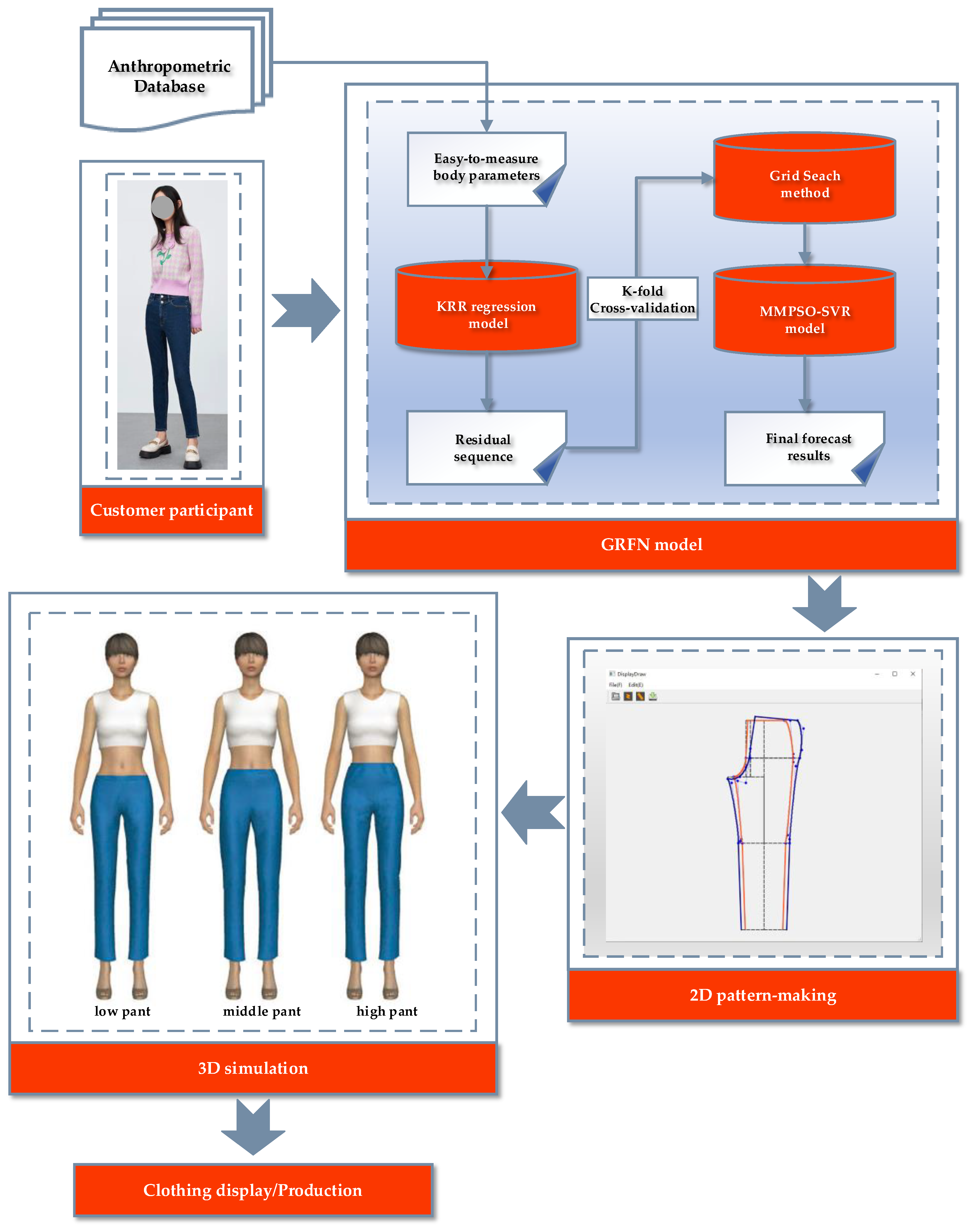
As shown in Figure 8A, a customer participant can input a few basic body parameters and accurately predict the relevant dimensions for pattern making via the GRFN. We also provide an interactive automatic pattern generation prototype, built using Microsoft Visual Studio 2013 and the Qt 5 integrated C++ development environment. Figure 8B depicts a screenshot of this system. During the pattern making process, a point-numbering method [53] is used to draw the structural lines of clothing patterns. The pattern for three-quarter, seven-quarter, and long pants are shown in Figure 8C. Utilizing the parameter settings of CLO Standalone virtual design software, a customer can effectively identify the precise measurement landmarks required based on the Chinese National Standard, namely GB 3975-1983 [54] and GB 16160-2017 [55], to construct an accurate human body model. Figure 8D illustrates the effect of this 3D simulation using an avatar.

4.5. Performance Comparison with Other Single Optimization SVR Methods

To verify the MMPSO model’s performance in optimizing the SVR hyperparameters, we select HCLDMSPSO-SVR, HCLPSO-SVR, PSO-LSSVM, and BPNN models for comparison. We set the MMPSO-SVR, HCLDMSPSO-SVR, HCLPSO-SVR, and PSO-LSSVM models to the maximum iteration limit of 1000, with a population size of 50. We selected the HCLDMSPSO [48] and HCLPSO [46] models as representative SOTA swarm-intelligence algorithms. We built a BPNN with an input layer consisting of five nodes. The hidden layer consisted of 13 nodes, and the output layer consisted of 8 nodes. The objective function was set to the minimum fitness value, and the best optimization result was preserved during the training process. To analyze the hyperparameter influence for an SVR small-sample human body size estimation, we compared the single MMPSO-SVR optimization model enhanced with the population’s diversity to avoid local optima in subsequent iterations, thus improving overall accuracy.

Based on our quantitative analysis, we compared each model’s prediction results, as shown in

Table 8. Comparison of estimation results of single optimization SVR models ($e_{RMSE}$ and $e_{MAE}$ in cm).

Algorithm	Item	${\mathit{e}}_{\mathit{R}\mathit{M}\mathit{S}\mathit{E}}\downarrow$	${\mathit{e}}_{\mathit{M}\mathit{A}\mathit{E}}\downarrow$	${\mathit{R}}^2\uparrow$	Item	${\mathit{e}}_{\mathit{R}\mathit{M}\mathit{S}\mathit{E}}\downarrow$	${\mathit{e}}_{\mathit{M}\mathit{A}\mathit{E}}\downarrow$	${\mathit{R}}^2\uparrow$
MMPSO-SVR	CH	1.5385	1.1225	0.8686	TCL	1.7991	1.2943	0.7794
HCLDMSPSO-SVR		1.5741	1.1335	0.8607		2.0060	1.5564	0.7243
HCLPSO-SVR		1.5709	1.1326	0.8609		2.0124	1.5222	0.7301
PSO-LSSVM		1.5915	1.1492	0.8568		2.0593	1.5325	0.7237
BPNN		2.1858	1.4342	0.7219		3.1221	2.2151	0.5894
MMPSO-SVR	KH	0.5804	0.4429	0.9774	AC	1.3579	1.0440	0.9721
HCLDMSPSO-SVR		0.6145	0.4360	0.9768		1.3936	1.0637	0.9708
HCLPSO-SVR		0.6105	0.4283	0.9765		1.3933	1.0621	0.9709
PSO-LSSVM		0.6109	0.4287	0.9765		1.4113	1.0769	0.9698
BPNN		0.6475	0.5337	0.9404		1.6073	1.2638	0.9661
MMPSO-SVR	TC	1.5479	1.3291	0.8602	KC	1.0930	0.8490	0.8212
HCLDMSPSO -SVR		1.5734	1.3450	0.8542		1.0932	0.8491	0.8210
HCLPSO-SVR		1.5666	1.3373	0.8547		1.0941	0.8635	0.8171
PSO-LSSVM		1.5732	1.3475	0.8539		1.0942	0.8512	0.8203
BPNN		1.8710	1.4267	0.7507		1.5102	1.1552	0.6559
MMPSO-SVR	CW	0.5604	0.3884	0.7428	AH	0.4899	0.3629	0.9923
HCLDMSPSO -SVR		0.5676	0.3972	0.7332		0.5016	0.4321	0.9883
HCLPSO-SVR		0.5655	0.3951	0.7356		0.5119	0.4232	0.9882
PSO-LSSVM		0.5671	0.4020	0.7309		0.5369	0.5603	0.9799
BPNN		0.5755	0.4521	0.7241		0.9344	0.6180	0.9709

Notes: $e_{RMSE}$ and $e_{MAE}$ in centimeters. Symbol $\downarrow$ represents that the smaller value, the better. Symbol $\uparrow$ represent that the larger value, the better. Values in bold font indicate the optimal results.

. By assessing the $R^2$ statistics, we concluded that the degree of fit for a single MMPSO-SVR model was the highest in all parts, and the $e_{RMSE}$ and $e_{MAE}$ measures were the smallest of all prediction methods. This again clearly demonstrates the effectiveness of our proposed single unmodified MMPSO-SVR global optimization model. Compared with other single optimization SVR hyperparameter methods, our method demonstrates superior efficacy by evading local optima and attaining the global optimum.

4.6. Ablation Experiments

To validate the accuracy and reliability of our proposed model, we conducted an ablation study by using two simplified models: our KRR regression version and our single direct MMPSO-SVR version. Figure 9A–H present the performance results on the few-shot human body dimension dataset. The comparative analysis involved assessing the predictive accuracy of the GRFN model in terms of the KRR regression and the single direct MMPSO-SVR models. Compared with the $e_{RMSE}$ values of the single direct MMPSO-SVR model, those of the combination hybrid model increased by 97.12% maximally in crotch width, and by 91.73% maximally in abdomen circumference. The $e_{RMSE}$ and $e_{MAE}$ values indicate that the hybrid model demonstrated superior predictive performance compared with every other model. The KRR regression model performed poorly in predicting $R^2$ values across all measurement items, but the single unmodified MMPSO-SVR achieved $R^2$ values above 0.9 for KH, AC, and AH predictions. However, it struggled with CW and TCL, which are particularly challenging to measure accurately, resulting in low $R^2$ values. In contrast, the regression values of our hybrid model were above 0.999 for all prediction items, indicating that our method predicts body sizes relevant to garment pattern making more accurately and efficiently, effectively avoiding the shortcomings of single body dimension prediction methods.

5. Discussion and Conclusions

With the rapid development of artificial intelligence technology, efficiently estimating the human body dimensions required for clothing patterns using ANN technology, rather than anthropometry measurement methods, has emerged as a new trend. The KRR regression model does not require feature selection and exhibits strong robustness to outliers, making it particularly suitable for handling datasets with noise or outliers. However, due to the ambiguity in the variable relationships among body dimensions, the KRR-based model may not fully capture their nonlinear features. Therefore, by enhancing the improved SVR model to compensate for the nonlinear features in the body dimension data, we have developed a nonlinear hybrid prediction approach with a high tolerance for input errors. This study employed an innovative data-driven GRFN hybrid model, based on a small-batch sample, for predicting highly accurate human body dimensions. We use the KRR regression model to fit and construct the predictive residual sequence. The MMPSO-SVR model is used to deal with nonlinear relationships and noisy data and to obtain more accurate predictive residual correction values. We then combine the estimated values from the KRR regression and the predictive residual correction values to obtain high-precision estimates of human body size parameters. Using the proposed teaching and learning co-optimization MMPSO algorithm enhances global search capabilities and population diversity [56], effectively preventing the algorithm from falling into local optima, thus leading to optimal SVR hyper-parameters. The experimental results validate the suitability of the proposed hybrid residual correction model, and compared with the performance of the single direct MMPSO-SVR model, the GRFN hybrid model exhibits astonishing improvements in RMSE of between 91.73% and 97.12%. Compared with the prediction accuracy and reliability results of other SOTA ANNs, those of our model are improved by 0.0054 ± 0.07 in terms of MSE and SE. The absolute error fluctuation range of the hybrid model is smaller than those of the other models. Hence, this remarkable advancement provides the fashion industry with intelligent garment design tools to effectively achieve the accuracy and efficiency of mass customization.

To further improve prediction accuracy and ease of implementation, we plan to overcome data limitations and improve the anthropometric dataset to cover full-body information, especially the anthropometric data of abnormal body shapes. Apart from the sample data capacity, we will also consider the impact of gender, age, ethnicity, geographical region, and body mass index on data sources. We also plan to improve the diversity of enhanced particle individuals in the MMPSO algorithm by leveraging the topological structure and communication methods of particles to improve global search stability and convergence.

References

1. Wu, G.; Liu, S.; Wu, X.; Ding, X. Research on lower body shape of late pregnant women in Shanghai area of China. Int. J. Ind. Ergon. 2015, 46, 69–75. [Google Scholar] [CrossRef]
2. Wang, L.; Lee, T.J.; Bavendiek, J.; Eckstein, L. A data-driven approach towards the full anthropometric measurements pre-diction via generalized regression neural networks. Appl. Soft Comput. 2021, 109, 107551. [Google Scholar] [CrossRef]
3. Su, J.; Ke, Y.; Kuang, C.; Gu, B.; Xu, B. Converting lower-body features from three-dimensional body images into rules for individualized pant patterns. Text. Res. J. 2019, 89, 2199–2208. [Google Scholar] [CrossRef]
4. Galada, A.; Baytar, F. Developing a prediction model for improving bifurcated garment fit for mass customization. Int. J. Cloth. Sci. Technol. 2023, 35, 397–418. [Google Scholar] [CrossRef]
5. Chan, A.P.; Fan, J.; Yu, W. Men’s shirt pattern design part II: Prediction of pattern parameters from 3D body measurements. J. Fiber Sci. Technol. 2003, 59, 328–333. [Google Scholar] [CrossRef]
6. Liu, K.; Wang, J.; Kamalha, E.; Li, V.; Zeng, X. Construction of a prediction model for body dimensions used in garment pattern making based on anthropometric data learning. J. Text. Inst. 2017, 108, 2107–2114. [Google Scholar] [CrossRef]
7. Liu, K.; Wu, H.; Zhu, C.; Wang, J.; Zeng, X.; Tao, X.; Bruniaux, P. An evaluation of garment fit to improve customer body fit of fashion design clothing. Int. J. Adv. Manuf. Technol. 2022, 120, 2685–2699. [Google Scholar] [CrossRef]
8. Cheng, P.; Chen, D.; Wang, J. Fast clustering of male lower body based on GA-BP neural network. Int. J. Cloth. Sci. Technol. 2020, 32, 163–176. [Google Scholar] [CrossRef]
9. Cheng, P.; Chen, D.; Wang, J. Research on underwear pressure prediction based on improved GA-BP algorithm. Int. J. Cloth. Sci. Technol. 2021, 33, 619–642. [Google Scholar]
10. Liu, Z.; Li, J.; Chen, G.; Lu, G. Predicting detailed body sizes by feature parameters. Int. J. Cloth. Sci. Technol. 2014, 26, 118–130. [Google Scholar] [CrossRef]
11. Wang, Z.; Wang, J.; Xing, Y.; Yang, Y.; Liu, K. Estimating human body dimensions using RBF artificial neural networks technology and its application in activewear pattern making. Appl. Sci. 2019, 9, 1140. [Google Scholar] [CrossRef]
12. Li, X.; Jing, X. The establishment of human body three vital measurements regression relationship based on SVR method. Int. J. Cloth. Sci. Technol. 2015, 27, 148–158. [Google Scholar] [CrossRef]
13. Rativa, D.; Fernandes, B.J.T.; Roque, A. Height and weight estimation from anthropometric measurements using machine learning regressions. IEEE J. Transl. Eng. Health Med. 2018, 6, 4400209. [Google Scholar] [CrossRef] [PubMed]
14. Li, T.; Lyu, Y.; Guo, Z.; Du, L.; Zou, F. Construction of the PSO-LSSVM prediction model for sleeve pattern dimensions based on garment flat recognition. Int. J. Cloth. Sci. Technol. 2023, 35, 67–87. [Google Scholar] [CrossRef]
15. Wang, Z.; Tao, X.; Zeng, X.; Xing, Y.; Xu, Y.; Xu, Z.; Bruniaux, P.; Wang, J. An interactive personalized garment design recommendation system using intelligent techniques. Appl. Sci. 2022, 12, 4654. [Google Scholar] [CrossRef]
16. Liu, X.; Wu, Y.; Wu, H. Machine learning enabled 3D body measurement estimation using hybrid feature selection and Bayesian search. Appl. Sci. 2022, 12, 7253. [Google Scholar] [CrossRef]
17. Wang, Z.; Tao, X.; Zeng, X.; Xing, Y.; Xu, Z.; Bruniaux, P. Design of customized garments towards sustainable fashion using 3D digital simulation and machine learning-supported human-product interactions. Int. J. Comput. Intell. Syst. 2023, 16, 16. [Google Scholar] [CrossRef]
18. Poli, R. Analysis of the publications on the applications of particle swarm optimisation. J. Artif. Evol. Appl. 2008, 2008, 685175. [Google Scholar] [CrossRef]
19. Liang, B.; Zhao, Y.; Li, Y. A hybrid particle swarm optimization with crisscross learning strategy. Eng. Appl. Artif. Intell. 2021, 105, 104418. [Google Scholar] [CrossRef]
20. Shi, Y.; Eberhart, R.C. Empirical study of particle swarm optimization. In Proceedings of the 1999 Congress on Evolutionary Computation-CEC99, Washington, DC, USA, 6–9 July 1999; pp. 1945–1950. [Google Scholar]
21. Chen, K.; Zhou, F.; Liu, A. Chaotic dynamic weight particle swarm optimization for numerical function optimization. Knowl.-Based Syst. 2018, 139, 23–40. [Google Scholar] [CrossRef]
22. Tian, D.; Shi, Z. MPSO: Modified particle swarm optimization and its applications. Swarm Evol. Comput. 2018, 41, 49–68. [Google Scholar] [CrossRef]
23. Mendes, R.; Kennedy, J.; Neves, J. The fully informed particle swarm: Simpler, maybe better. IEEE Trans. Evol. Comput. 2004, 8, 204–210. [Google Scholar] [CrossRef]
24. Liang, J.J.; Suganthan, P.N. Dynamic multi-swarm particle swarm optimizer. In Proceedings of the 2005 IEEE Swarm Intelligence Symposium, Pasadena, CA, USA, 8–10 June 2005; pp. 124–129. [Google Scholar]
25. Lim, W.H.; Mat Isa, N.A. An adaptive two-layer particle swarm optimization with elitist learning strategy. Inf. Sci. 2014, 273, 49–72. [Google Scholar] [CrossRef]
26. Liang, J.J.; Qin, A.K.; Suganthan, P.N.; Baskar, S. Comprehensive learning particle swarm optimizer for global optimization of multimodal functions. IEEE Trans. Evol. Comput. 2006, 10, 281–295. [Google Scholar] [CrossRef]
27. Wang, H.; Wu, Z.; Rahnamayan, S.; Liu, Y.; Ventresca, M. Enhancing particle swarm optimization using generalized opposition-based learning. Inf. Sci. 2011, 181, 4699–4714. [Google Scholar] [CrossRef]
28. Zhan, Z.; Zhang, J.; Li, Y.; Shi, Y. Orthogonal learning particle swarm optimization. IEEE Trans. Evol. Comput. 2011, 15, 832–847. [Google Scholar] [CrossRef]
29. Xu, G.; Cui, Q.; Shi, X.; Ge, H.; Zhan, Z.-H.; Lee, H.P.; Liang, Y.; Tai, R.; Wu, C. Particle swarm optimization based on dimensional learning strategy. Swarm Evol. Comput. 2019, 45, 33–51. [Google Scholar] [CrossRef]
30. Wolpert, D.H.; Macready, M.G. No free lunch theorems for optimization. IEEE Trans. Evol. Comput. 1997, 1, 67–82. [Google Scholar] [CrossRef]
31. Lu, J.; Zhang, J.; Sheng, J. Enhanced multi-swarm cooperative particle swarm optimizer. Swarm Evol. Comput. 2022, 69, 100989. [Google Scholar] [CrossRef]
32. Yin, R.; Liu, Y.; Wang, W.; Meng, D. Sketch kernel ridge regression using circulant matrix: Algorithm and theory. IEEE Trans. Neural Netw. Learn. Syst. 2020, 31, 3512–3524. [Google Scholar] [CrossRef]
33. Liu, Y.; Liao, S.; Lin, Y.; Wang, W. Infinite kernel learning: Generalization bounds and algorithms. In Proceedings of the 31st AAAI Conference on Artificial Intelligence, San Francisco, CA, USA, 4–9 February 2017; pp. 2280–2286. [Google Scholar]
34. Li, S.; Fang, H.; Liu, X. Parameter optimization of support vector regression based on sine cosine algorithm. Expert Syst. Appl. 2018, 91, 63–77. [Google Scholar] [CrossRef]
35. Gu, X.; Xiao, Z. Research on the application of ARIMA-SVR combination model in satellite telemetry parameter prediction. Chin. J. Space Sci. 2022, 42, 306–312. [Google Scholar]
36. Yu, Y.; Gao, S.; Cheng, S.; Wang, Y.; Song, S.; Yuan, F. CBSO: A memetic brain storm optimization with chaotic local search. Memetic Comput. 2018, 10, 353–367. [Google Scholar] [CrossRef]
37. Tong, X.; Choi, K.; Lai, T.; Wong, W. Stability bounds and almost sure convergence of improved particle swarm optimization methods. Res. Math. Sci. 2021, 8, 30. [Google Scholar] [CrossRef]
38. Li, Z.; Wang, W.; Yan, Y.; Li, Z. PS-ABC: A hybrid algorithm based on particle swarm and artificial bee colony for high-dimensional optimization problems. Expert Syst. Appl. 2015, 42, 8881–8895. [Google Scholar] [CrossRef]
39. Zervoudakis, K.; Tsafarakis, S. A mayfly optimization algorithm. Comput. Ind. Eng. 2020, 145, 106559. [Google Scholar] [CrossRef]
40. Wu, Q.; Lin, H.; Jin, Y.; Chen, Z.; Li, S.; Chen, D. A new fallback beetle antennae search algorithm for path planning of mobile robots with collision-free capability. Soft Comput. 2020, 24, 2369–2380. [Google Scholar] [CrossRef]
41. He, Q.; Lin, J.; Xu, H. Hybrid cauchy mutation and uniform distribution of grasshopper optimization algorithm. Control Decis. 2021, 36, 1558–1568. [Google Scholar]
42. GB/T 1335.2-2008; Standard Sizing Systems for Garment-Women. GB/T: Beijing, China, 2008.
43. Liu, K.; Zhu, C. Clothing Intelligent Design: Structural Design and Fit Evaluation; China Textile Press: Beijing, China, 2021; pp. 138–141. [Google Scholar]
44. Suganthan, P.N.; Hansen, N.; Liang, J.J.; Deb, K.; Chen, Y.; Auger, A.; Tiwari, S. Problem definitions and evaluation criteria for the CEC 2005 special session on real-parameter optimization. In Proceedings of the 2005 IEEE Congress on Evolutionary Computation, Edinburgh, UK, 2–5 September 2005; pp. 1–50. [Google Scholar]
45. Peram, K.; Veeramachaneni, K.; Mohan, C.K. Fitness-distance-ratio based particle swarm optimization. In Proceedings of the IEEE Swarm Intelligence Symposium, Indianapolis, IN, USA, 24–26 April 2003; pp. 174–181. [Google Scholar]
46. Lynn, N.; Suganthan, P.N. Heterogeneous comprehensive learning particle swarm optimization with enhanced exploration and exploitation. Swarm Evol. Comput. 2015, 24, 11–24. [Google Scholar] [CrossRef]
47. Lynn, N.; Suganthan, P.N. Ensemble particle swarm optimizer. Appl. Soft Comput. 2017, 55, 533–548. [Google Scholar] [CrossRef]
48. Wang, S.; Liu, G.; Gao, M.; Cao, S.; Guo, A.; Wang, J. Heterogeneous comprehensive learning and dynamic multi- swarm particle swarm optimizer with two mutation operators. Inf. Sci. 2020, 540, 175–201. [Google Scholar] [CrossRef]
49. Varna, F.T.; Husbands, P. HIDMS-PSO: A New Heterogeneous Improved Dynamic Multi-Swarm PSO Algorithm. In Proceedings of the IEEE Symposium Series on Computational Intelligence (IEEE SSCI), Electr Network, Canberra, Australia, 1–4 December 2020; pp. 473–480. [Google Scholar]
50. Derrac, J.; García, S.; Molina, D.; Herrera, F. A practical tutorial on the use of nonparametric statistical tests as a methodology for comparing evolutionary and swarm intelligence algorithms. Swarm Evol. Comput. 2011, 1, 3–18. [Google Scholar] [CrossRef]
51. Zhou, X.; Zhou, S.; Han, Y.; Zhu, S. Levy flight-based inverse adaptive comprehensive learning particle swarm optimization. Math. Biosci. Eng. 2022, 19, 5241–5268. [Google Scholar] [CrossRef] [PubMed]
52. GB/T 23698-2009; General Requirements for 3-D Scanning Anthropometric Methodologies. GB/T: Beijing, China, 2009.
53. Liu, D. Clothing Pattern Design, 4th ed.; China Textile Press: Beijing, China, 2019; pp. 166–170. [Google Scholar]
54. GB 3975-1983; Terminology for Human Body Measurements. GB: Beijing, China, 1983.
55. GB/T 16160-2017; Anthropometric Definitions and Methods for Garment. GB/T: Beijing, China, 2007.
56. Kadirkamanathan, V.; Selvarajah, K.; Fleming, P.J. Stability analysis of the particle dynamics in particle swarm optimizer. IEEE Trans. Evol. Comput. 2006, 10, 245–255. [Google Scholar] [CrossRef]
Figure 1. Architecture of the GRFN model for human body dimension prediction. (In the 2D pattern-making subfigure, the blue curve represents the back pattern piece of the pant; the red curve represents the frontal pattern piece of the pant; the black curve indicates an auxiliary line. Additionally, the blue dots are used to denote auxiliary frames.)
Applsci 13 10317 g001
Figure 2. Full hybrid prediction process.
Applsci 13 10317 g002
Figure 3. The average ranking of PSO variants: (A) average ranking in unimodal functions of PSO variants; (B) average rank in multimodal and expanded functions of PSO variants.
Applsci 13 10317 g003
Figure 4. Critical difference under Friedman test, statistical rank.
Applsci 13 10317 g004
Figure 5. Comparison of MAE and RMSE with different input training samples; (A) crotch-height, (B) knee circumference.
Applsci 13 10317 g005
Figure 6. Predicted results of GRFN hybrid model; (A) crotch-height, (B) knee circumference.
Applsci 13 10317 g006
Figure 7. More results for body part prediction; (A) total crotch length, (B) crotch width, (C) thigh circumference, and (D) knee height.
Applsci 13 10317 g007
Figure 8. Pattern making and virtual simulation using body dimensions predicted by the GRFN model: (A) GRFN model, (B) 2D pattern making, (C) pant pattern, and (D) 3D simulation try-on. (Notes: In subfigure (B), the blue curve represents the back pattern piece of the pant; the red curve represents the frontal pattern piece of the pant; the black dot curve indicates an auxiliary line.)
Applsci 13 10317 g008
Figure 9. Performance comparison of regression model on small-sample body dimensions datasets: (A) crotch height; (B) total crotch length; (C) knee height; (D) abdomen circumference; (E) thigh circumference; (F) knee circumference; (G) crotch width; and (H) abdomen height.
Applsci 13 10317 g009