Abstract
The Earth’s synthetic gravitational and density models can be used to validate numerical procedures applied for global (or large-scale regional) gravimetric forward and inverse modeling. Since the Earth’s lithospheric structure is better constrained by tomographic surveys than a deep mantle, most existing 3D density models describe only a lithospheric density structure, while 1D density models are typically used to describe a deep mantle density structure below the lithosphere-asthenosphere boundary. The accuracy of currently available lithospheric density models is examined in this study. The error analysis is established to assess the accuracy of modeling the sub-lithospheric mantle geoid while focusing on the largest errors (according to our estimates) that are attributed to lithospheric thickness and lithospheric mantle density uncertainties. Since a forward modeling of the sub-lithospheric mantle geoid also comprises numerical procedures of adding and subtracting gravitational contributions of similar density structures, the error propagation is derived for actual rather than random errors (that are described by the Gauss’ error propagation law). Possible systematic errors then either lessen or sum up after applying particular corrections to a geoidal geometry that are attributed to individual lithospheric density structures (such as sediments) or density interfaces (such as a Moho density contrast). The analysis indicates that errors in modeling of the sub-lithospheric mantle geoid attributed to lithospheric thickness and lithospheric mantle density uncertainties could reach several hundreds of meters, particularly at locations with the largest lithospheric thickness under cratonic formations. This numerical finding is important for the calibration and further development of synthetic density models of which mass equals the Earth’s total mass (excluding the atmosphere). Consequently, the (long-to-medium wavelength) gravitational field generated by a synthetic density model should closely agree with the Earth’s gravitational field.
1. Introduction
Gravimetric forward and inverse modeling techniques are essential numerical tools applied in physical geodesy and gravimetric geophysics. In physical geodesy applications, these methods are used to compute topographic and terrain gravity corrections in gravimetric geoid modeling [1,2,3,4,5,6,7,8,9,10,11] and compile isostatic gravity maps [12]. In gravimetric geophysics, these methods are used to compile Bouguer and mantle gravity maps [13,14,15,16,17,18]. Furthermore, numerous techniques have been developed and applied for a gravimetric interpretation of the Earth’s inner structure [19,20,21].
Whereas gravimetric inverse modeling is applied to determine an unknown density structure or density interface from observed gravity data, gravimetric forward modeling is used to compute gravitational field quantities generated by a known density structure or density interface. Several different methods have been developed for local and regional gravimetric forward modeling based on solving Newton’s volume integral in the spatial domain by applying numerical, semi-analytical, and analytical methods [2,22,23,24,25,26,27,28,29,30,31,32]. In global (and large-scale regional) applications, methods of solving Newton’s volume integral in the spectral domain utilize a spherical harmonic analysis and synthesis of gravity and density structure models [33,34,35,36,37,38,39,40,41,42].
The validation of the accuracy and numerical efficiency of newly developed methods for gravimetric forward and inverse modeling is often performed by comparing results with solutions obtained from existing (and typically well-established) numerical methods and procedures. Alternatively, simple or more refined synthetic density models (designed for various configurations of different geometrical density bodies) have been more recently used for testing and validation of spatial methods developed for local and regional gravimetric forward modeling and inversion by adopting a planar approximation. For global (or large-scale regional) applications, synthetic density models should mimic more realistically the Earth’s actual shape and inner density structure. Such synthetic density models have already been used to validate numerical techniques involved in gravimetric geoid modeling [43,44,45], studies of the sediment bedrock morphology [46], the lithospheric and mantle density structure [16,47], the crustal thickness [16,18,47,48,49,50,51,52], the dynamic and residual topography [53,54,55], or the oceanic lithosphere [56]. To construct a global synthetic density model that closely resembles the Earth’s shape and inner structure, available global topographic and density structure models could be used for this purpose, together with additional models that provide information about the Earth’s inner structure (such as crust and lithospheric thickness models). Moreover, constraints have to be applied so that the mass of the Earth’s synthetic model is equal to the total mass of the Earth (excluding the atmosphere), and the gravitational field generated by the Earth’s synthetic model closely agrees with the Earth’s gravitational field (in terms of geoidal geometry, gravity, and gravity gradient).
A number of seismic velocities and mass density models have been developed based on the analysis of tomographic data while incorporating geophysical, geochemical, and geothermal constraints [57,58,59,60,61,62,63,64]. For an overview of these models, see also Trabant [65]. A practical application of global 1D density models [58,64] is limited by the absence of lateral density information. To address this issue, existing 2D or 3D crust and lithospheric models [66,67,68,69,70,71,72,73] can be used to refine 1D reference density models.
Since many parts of the world are not yet sufficiently covered by tomographic surveys, the refinement of 1D reference density models by incorporating 2D or 3D global lithospheric and mantle density models is not simple. Moreover, the direct relation between seismic velocities and mass densities does not exist because a density distribution depends on many other factors (such as temperature, mineral composition, and pressure). In spite of these practical and theoretical limitations, the development of synthetic density models that more or less realistically approximate the Earth’s shape and inner density structure is essential for a more comprehensive assessment of gravimetric forward and inverse modeling techniques (than those based on using simplistic, typically geometric density models). Moreover, input data uncertainties should be known in order to realistically assess the accuracy of synthetic density models.
To inspect the possibilities of refining the Earth’s synthetic density model, the accuracy of published lithospheric density models is assessed based on a novel approach presented in this study. Whereas the accuracy of crustal density models has been partially inspected, a robust analysis of lithospheric mantle density models is absent. This novel approach allows us to formulate the error propagation and consequently provide rough error estimates in gravimetric forward modeling that are attributed to lithospheric density and geometry uncertainties. Gravimetric forward modeling is applied to determine a long-wavelength geoidal geometry that is corrected for the gravitational contributions of lithospheric density and thickness variations. Expressions for gravimetric forward modeling are presented in Section 2 and then used to derive the error analysis in Section 3. Numerical results are briefly presented in Section 4, and the accuracy of the results is discussed in Section 5. Major findings are concluded in Section 6.
2. Numerical Model
We applied methods for a spherical harmonic analysis and synthesis of gravitational and lithospheric density models to compute the sub-lithospheric mantle geoid. Details on theoretical aspects are given below.
2.1. Geoid
The geoid height is defined by the following [74]:
where the disturbing potential (i.e., the difference between values of the actual and normal gravity potential and , respectively; ) is stipulated at the geoid surface . The normal gravity in Equation (1) is computed at the ellipsoid surface according to Somigliana–Pizzetti’s theory [75,76] for the GRS80 [77] parameters. The 3D position in Equation (1) and thereafter is defined in the spherical coordinate system , where is the radius and denotes the spherical direction with the spherical latitude and longitude . In the context of interpreting long-wavelength features in the geoidal geometry attributed to a sub-lithospheric mantle density structure, the disturbing potential in Equation (1) can approximately (cf. Wieczorek [19,78]; Tenzer et al. [79]) be computed by using the following expression [74]:
where m3·s−2 is the geocentric gravitational constant, m is the Earth’s mean radius, are the (fully-normalized) disturbing potential coefficients, are the (fully-normalized) surface spherical functions of degree n and order m, and is the upper summation index of spherical harmonics.
2.2. Sub-Lithospheric Mantle Geoid
In the forward modeling scheme, the gravitational contribution of lithospheric density heterogeneities is subtracted from a geoidal geometry in order to enhance the gravitational signature of density structures within the mantle below the lithosphere (i.e., within the sub-lithospheric mantle). This procedure yields the sub-lithospheric mantle geoid , defined by the following:
The computation of the sub-lithospheric mantle disturbing potential in Equation (3) is realized in numerical steps, as explained next.
2.2.1. Bouguer Disturbing Potential
The Bouguer disturbing potential is obtained from the disturbing potential after subtracting the gravitational potentials of topography , bathymetry , and polar glaciers . We then write the following (cf. Tenzer et al. [48,50]):
The gravitational potentials of atmosphere [80] and lakes [81] are completely negligible when compared to values of the gravitational potentials , , and .
The topographic potential in Equation (4) is often computed individually for a uniform and anomalous topographic density. The topographic potential for a uniform topographic density reads as follows [12]:
The potential coefficients in Equation (5) are given by the following:
where kg·m−3 is the Earth’s mean mass density, and is the average (constant) topographic density. The Laplace harmonics of topographic heights are defined by the following integral convolution:
where are the topographic coefficients, is the Legendre polynomial for the argument of cosine of the spherical angle between two points and ; i.e., . The infinitesimal surface element on the unit sphere is denoted as , and is the full spatial angle. The corresponding higher-order terms {} read as follows:
The topographic potential for an anomalous lateral topographic density is computed from the following:
where
The topographic density-heights coefficients {} in Equation (10) are given by the following:
The height in Equation (11) equals the topographic height , except for areas covered by polar glaciers. In this case, the height is defined as the topographic height minus the ice thickness. The anomalous lateral topographic density in Equation (11) is taken with respect to the average topographic density , so that .
The bathymetric potential in Equation (4) is defined by the following [82,83]:
The bathymetric coefficients read as follows:
where is the nominal value of the surface seawater density contrast, and , , and denote parameters of the depth-dependent seawater density developed by Gladkikh and Tenzer [84]. The numerical coefficients , , and in Equation (13) are computed from the following:
The coefficients of global bathymetric model are defined by the following:
and their higher-order terms read (ibid.) as follows:
where denotes the bathymetric depth.
The ice potential in Equation (4) is computed from (cf. Foroughi and Tenzer [85]) as follows:
The ice coefficients in Equation (19) read as follows:
where the numerical coefficients and are given by the following:
The coefficients utilize the spherical lower-bound functions of a volumetric mass density contrast layer and their higher-order terms [82,83]:
Since the upper-bound of glaciers is identical with the topographic surface, the numerical coefficients are generated directly from the height coefficients {}. The ice density contrast in Equation (20) is taken with respect to a uniform topographic density , i.e., , where denotes the density of polar glaciers.
2.2.2. Crust-Stripped Disturbing Potential
The gravitational potential of consolidated-crust density contrast and the gravitational potential of sediment density contrast are subtracted from the Bouguer disturbing potential in order to remove the gravitational contribution of density heterogeneities within the whole crust. This procedure yields the crust-stripped disturbing potential (cf. Tenzer et al. [48]):
The potentials and in Equation (23) are computed according to a method developed by Tenzer et al. [82] that utilizes the expression for a gravitational potential generated by an arbitrary volumetric mass layer with a variable depth and thickness while having laterally distributed vertical mass density variations. It reads as follows:
The potential coefficients in Equation (24) are defined by the following
where the coefficients {} are computed from the following:
The terms and in Equation (26) define the spherical lower-bound and upper-bound laterally distributed radial density variation functions and of degree . These numerical coefficients combine information on the geometry and mass density (or density contrast) distribution within a volumetric layer. The computation of these coefficients is realized to a certain degree in spherical harmonics from discrete data of the spatial mass density distribution (typically provided by means of density, depth, and thickness data) of a particular structural component of the Earth’s interior.
The spherical functions and , including their higher-order terms {} in Equation (26), are defined by the following:
and
For a specific volumetric layer, the mass density is either constant , laterally varying , or—in the most general case—approximated by the laterally distributed radial density variation model by using the following polynomial function (for each lateral column):
The nominal value of lateral density is stipulated at the depth . This density distribution describes a radial density variation, in terms of coefficients {} and , within a volumetric mass layer at a location . Alternatively, when modeling a gravitational field of anomalous density structures (in this case, the density contrast of sediments and consolidated crust), the density contrast of volumetric mass layer relative to the reference density is defined by the following:
where is the nominal value of lateral density contrast stipulated at the depth . Here, the reference density of homogenous crust is used.
2.2.3. Mantle Disturbing Potential
To reveal a gravitational signature attributed to a mantle density structure, the Moho geometry signature has to be subtracted from the crust-stripped disturbing potential. This procedure yields the mantle disturbing potential. According to Tenzer et al. [50], the mantle disturbing potential is obtained from the crust-stripped disturbing potential after subtracting the gravitational potential of Moho geometry . We then write the following:
The potential (for the average Moho density contrast ) is defined in the following form:
where the numerical coefficients are given by the following:
The Moho depth spherical functions and their higher-order terms {} read as follows:
As seen in Equation (34), the coefficients {} are generated from values of the Moho depth . The Moho density contrast in Equation (33) is defined as the average lithospheric mantle density from which the (constant) reference crustal density is subtracted. Hence,
2.2.4. Lithosphere-Stripped Disturbing Potential
The lithosphere-stripped disturbing potential is obtained from the mantle disturbing potential after subtracting the lithospheric-mantle gravitational potential . We then write the following:
For a lateral density distribution function within the lithospheric mantle, the lithospheric-mantle gravitational potential is defined by the following:
where the Moho coefficients describe the geometry and lateral density (contrast) distribution at the Moho interface, and the LAB coefficients describe the geometry and lateral density (contrast) distribution at the LAB.
The Moho coefficients in Equation (37) are defined in the following form:
where denotes the Moho depth (see Equation (34)). The (lateral) lithospheric mantle density contrast in Equation (38) is computed as the difference between the adopted (lithospheric mantle) reference density and the lithospheric mantle density ; i.e., .
The LAB coefficients in Equation (37) read as follows:
where is the LAB depth. If we consider a current resolution of global lithospheric density models (1 × 1 arc-deg or lower) that corresponds (by means of a half wavelength) to a spectral resolution up to the degree 180 of spherical harmonics, the lithospheric-mantle gravitational potential can sufficiently be computed by using a binomial series in Equation (37) up to only the third-order term.
2.2.5. Sub-Lithospheric Mantle Disturbing Potential
The computation of the lithosphere-stripped disturbing potential in Equation (36) enhanced a signature of the LAB geometry that has to be removed in order to enhance a gravitational signature of the sub-lithospheric mantle density structure. This procedure is realized by stripping the lithosphere with respect to the density contrast between the reference (lithospheric mantle) density and the asthenosphere density in order to obtain the sub-lithospheric mantle disturbing potential. The sub-lithospheric mantle disturbing potential is then computed as follows:
where the potential of LAB geometry is defined by the following:
The coefficients in Equation (41) read as follows:
where is the LAB depth (see also Equation (39)), and the LAB density contrast is defined as the difference between the lithospheric mantle density and the asthenospheric density . We note that the computation of can again be restricted up to the third-order terms of a binomial series (as in the case of computing in Equation (37)).
3. Model Uncertainties
The numerical model presented in Section 2 was used in this section to derive the error propagation in the modeling of the sub-lithospheric mantle geoid. The gravitational contributions of the lithospheric mantle and LAB are one order of magnitude larger than the corresponding contributions of topographic and crustal density structures. We, therefore, focused only on the estimation of errors due to lithospheric mantle density and lithospheric thickness uncertainties while disregarding much smaller (in an absolute sense) modeling errors due to crustal density uncertainties.
3.1. Errors Due to Lithospheric Thickness Uncertainties
In sub-lithospheric mantle geoid modeling, the lithospheric thickness information is used to compute the lithospheric-mantle gravitational potential (in Equation (39)) and the LAB potential (in Equation (41)). We then established a relation between the error of sub-lithospheric mantle geoid and the error of lithospheric thickness in the following form:
After disregarding terms , the expression in Equation (43) simplifies to the following:
For n = 0, we have the following:
When assuming that the largest contribution to the error comes from lithospheric thickness uncertainties in the vicinity of the computation point (for which the error is estimated), the global integration domain in Equation (45) could be disregarded. Instead, we reduce a functional relation only for a position of computation point. We then write the following:
Inserting for in Equation (46), we arrive at the following:
3.2. Errors Due to Lithospheric Mantle Density Uncertainties
The lithospheric mantle density information is used to compute the Moho density contrast in Equation (35), the lithospheric mantle density variations in Equation (38), and the LAB density contrast in Equation (42). This involves the computation of the Moho potential in Equation (32), the lithospheric-mantle gravitational potential in Equation (39), and the LAB potential in Equation (41). The error propagation for the lithospheric mantle density uncertainties is then established in the following form:
where , , and denote, respectively, the errors in the Moho density contrast , the anomalous lithospheric mantle density , and the LAB density contrast .
After disregarding terms in Equation (48), we arrive at the following:
Considering that n = 0 and , we obtain the following:
By analogy with Equation (46), the expression in Equation (50) is further simplified to the following:
As seen in Equation (51), the sub-lithospheric mantle geoid error in this case depends on the accuracy of the anomalous lithospheric mantle density . In addition, the errors and in adopted values of the LAB density contrast and the Moho density contrast affect the accuracy.
4. Results
Tenzer and Chen [81] applied numerical procedures (described in Section 2) to compute the global sub-lithospheric mantle geoid globally with a spectral resolution up to degree 180 of spherical harmonics. They used the EIGEN-6C4 [86] global gravitational model, the Earth2014 topographic, bathymetric, and glacial bedrock relief datasets [72], the UNB_TopoDens global lateral topographic density model [87], the total sediment thickness data for the world’s oceans and marginal seas [88], the CRUST1.0 [69] global seismic crustal model updated for the sediment and crustal layers of the Antarctic lithosphere by Baranov et al. [89], and the LITHO1.0 [70] global seismic lithospheric model. They adopted the reference density values of 2670 kg·m−3 (cf. Hinze [90]; Artemjev et al. [91]) for the crust above the geoid, 2900 kg·m−3 for the crust below the geoid, and 3300 kg·m−3 for the lithospheric mantle. To further improve the accuracy of forward modeling, they defined the ocean density contrast for a depth-dependent seawater density function [47,84] and applied a density model of marine sediments [92] under marginal seas and oceans.
Gravitational contributions of individual lithospheric density structures are plotted in Figure 1, with the statistical summary of results in Table 1. Modifications of the geoidal geometry after subtracting the gravitational contributions of individual lithospheric density structures are presented in Figure 2, with the statistical summary in Table 2.
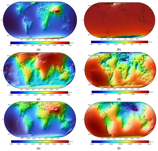
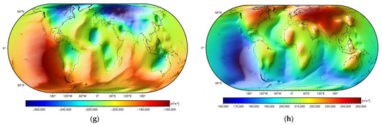
Figure 1.
Global maps of the gravitational potentials of (a) topography , (b) ice , (c) bathymetry , (d) sediments , (e) consolidated crust , (f) Moho geometry , (g) lithospheric mantle , and (h) LAB geometry .

Table 1.
Statistics of gravitational potentials used to compute the sub-lithospheric mantle gravity disturbances. For the notation used, see the legend in Figure 1.
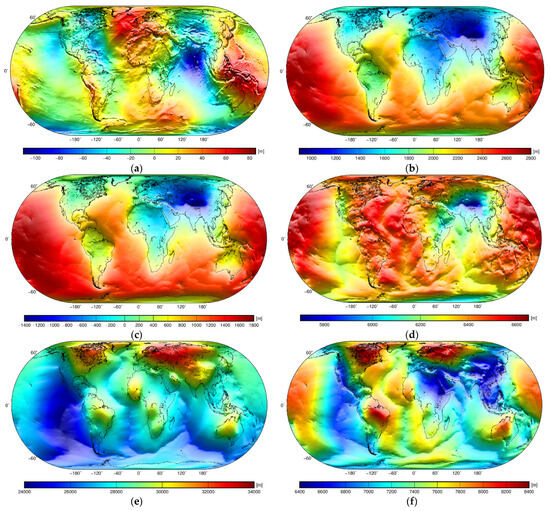
Figure 2.
Global maps of (a) the geoid , (b) the Bouguer geoid , (c) the crust-stripped geoid , (d) the mantle geoid , (e) the lithosphere-stripped geoid , and (f) the sub-lithospheric mantle geoid .
Table 2.
Statistics of geoid models. For the notation used, see the legend in Figure 2.
A long-wavelength geoidal geometry (Figure 2a) reflects mainly a mantle density structure [93,94], while a signature of crustal density and geometry variations (including a topographic surplus of large orogenic formations) is less prominent. After removing the gravitational contributions of topography and lithospheric density and geometry (i.e., LAB) variations, the resulting (sub-lithospheric mantle) geoidal geometry (see Figure 2f) should (optimally) enhance the gravitational signature of the sub-lithospheric mantle.
It is a well-known fact that a spatial pattern in dynamic topography models [54,55,95,96,97,98] mainly reflects a mantle convection flow, with maxima marking locations of the African and South Pacific superplumes that represent large-scale regions characterized by an elevated topography and shallow ocean-floor depths caused by a low-density upwelling of mantle material from the core-mantle boundary. The corresponding minima are explained by a high-density mantle downwelling flow. Tomographic studies [99] indicate that superplumes coincide with the locations of large low-shear-velocity provinces (LLSVPs) beneath Africa (called Tuzo) and the South Pacific (called Jason). Since the gravitational contributions of lithospheric density and thickness variations have been modeled and consequently removed in our forward modeling procedure, the sub-lithospheric mantle geoid should mainly reflect deep mantle density anomalies. Consequently, the spatial pattern of the sub-lithospheric mantle geoid (especially its long-wavelength spectrum up to degree five of spherical harmonics; see Figure 3) does not closely agree with the spatial pattern of dynamic topography models (cf. Tenzer and Chen [81]). A comparative study of spatial patterns in the sub-lithospheric mantle geoid and dynamic topography models is thus not meaningful for the assessment of errors in our gravimetric forward modeling.
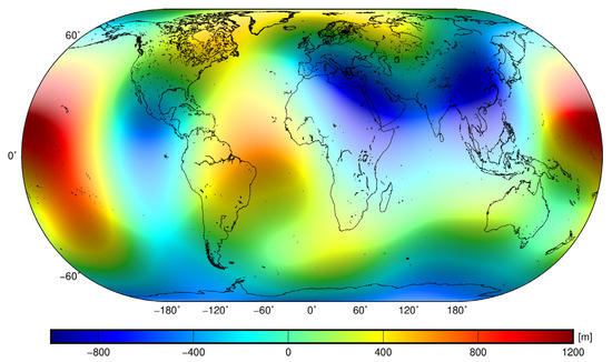
Figure 3.
The sub-lithospheric mantle geoid is computed up to degree 5 of spherical harmonics (and calibrated so its mean value equals zero).
As seen in Figure 3, the long-wavelength pattern in the sub-lithospheric mantle geoid is characterized by a large positive anomaly in the Central Pacific and a less pronounced anomaly in the Central Atlantic, with a prolonged shape across the Atlantic Ocean and further extending across the South Indian Ocean towards West Australia. These two positive anomalies are coupled with negative anomalies in the Equatorial East Pacific and across South and East Eurasia. An additional negative anomaly was detected in Antarctica. If we consider that a spatial pattern of the sub-lithospheric mantle geoid should mainly manifest sub-lithospheric mantle density heterogeneities, it becomes clear that a long-wavelength pattern in Figure 3 might be affected by large errors, especially at locations with a maximum lithospheric thickness. This becomes even more evident when inspecting the sub-lithospheric mantle geoid in Figure 2f, where a maximum lithospheric deepening is clearly manifested in the geoidal geometry. This indicates the possible presence of large errors attributed to the lithospheric model uncertainties used in the gravimetric forward modeling. These errors are estimated in the next section.
5. Error Analysis
Large errors are expected in the CRUST1.0 and LITHO1.0 models used for gravimetric forward modeling in this study. As already mentioned in the preceding section, this is particularly evident from pronounced positive sub-lithospheric mantle geoid anomalies (Figure 2f) that are also still partially exhibited in their long-wavelength pattern (Figure 3). These positive anomalies correspond with the largest cratonic lithospheric thickness (the Laurentian Shield in North America, the Amazonian Shield and São Francisco Craton in South America, the West African Craton, the East European and Siberian Cratons, the Baltic Shield in Eurasia, and the West Australian Craton).
As seen in Equation (47), the lithospheric thickness uncertainties propagate almost linearly to the sub-lithospheric mantle geoid uncertainties. We can, therefore, readily estimate the geoid errors for particular lithospheric thickness uncertainties. According to the LITHO1.0 model, the lithospheric mantle density varies roughly from 3000 to 3450 kg·m−3. From these density variations, we can assume that is mostly within ±200 kg·m−3. The boundary between the lowermost lithosphere and the uppermost asthenosphere (i.e., the LAB) is rheological, conventionally taken at the 1300 °C isotherm, above which the mantle behaves in a rigid fashion and below which it behaves in a ductile fashion [100]. Studies suggest the existence of a compositional or chemical density contrast 0–20 kg·m−3 [101], except probably the cratonic mantle. In addition to a possibly chemical density contrast, a strong thermal density contrast of 30–60 kg·m−3 occurs when the asthenosphere is locally uplifted by rifting. We, therefore, assume that the density variations at the boundary between the lithosphere and the asthenosphere are mostly within ±30 kg·m−3. For kg·m−3, the errors in the lithospheric thickness estimates of km cause errors in the sub-lithospheric mantle geoid of roughly km.
The lithospheric thickness models vary significantly. Pasyanos et al. [70], for instance, found large differences between their LITHO1.0 model and that prepared by Conrad and Lithgow–Bertelloni [102]. They also explained that these large differences are due to applying different methods, assumptions, and input data. To get a rough idea about the magnitude of these errors, we compared the lithospheric thickness models SLNAAFSA [103], SL2013sv [104], LITHO1.0 [70], CAM2016 [105,106], and 3D2015-07Sv [107], and used their differences to estimate (sub-lithospheric mantle) geoid errors. We note here that the SLNAAFSA model was prepared by Hoggard et al. [103] by merging regional updates from North America [108], Africa [109], and South America [110] into the global SL2013sv model. The lithospheric thickness models are shown in Figure 4, with their statistical summary given in Table 3. The statistics of differences between individual lithospheric thickness models are summarized in Table 4.
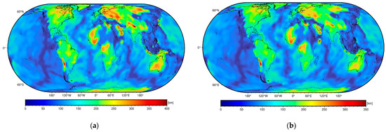
Figure 4.
Lithospheric thickness models: (a) SLNAAFSA, (b) SL2013sv, (c) LITHO1.0, (d) CAM2016, and (e) 3D2015-07Sv.
Table 3.
Statistics of the lithospheric thickness models SLNAAFSA, SL2013sv, LITHO1.0, CAM2016, and 3D2015-07Sv.
Table 4.
Statistics of differences between the lithospheric thickness models.
As seen in Table 4, differences between lithospheric thickness models exceed several hundreds of meters. If we consider that the average uncertainties in the lithospheric thickness are about ±40 km (the average of the root-mean-square (RMS) of differences in Table 4), the sub-lithospheric mantle geoid errors could reach or even exceed ±0.4 km.
Tomographic images of the lithosphere have limited accuracy and resolution. Moreover, the conversion between seismic wave velocities and rock densities is not unique [58,111]. Hager and Richards [112], for instance, mentioned that a lithospheric mantle composition and seismic anisotropy are more complex than a deep mantle structure, making it harder to convert seismic anomalies to density anomalies or buoyancy (cf. also Simmons et al. [113]). We, therefore, also expect large (sub-lithospheric mantle) geoid modeling errors due to lithospheric mantle density uncertainties.
According to Equation (51), the sub-lithospheric mantle geoid error depends on the accuracy of anomalous lithospheric mantle density and additional errors and in adopted values of the LAB density contrast and the Moho density contrast . Large density variations occur within the lithospheric mantle, although in comparison to the crust, fewer constraints exist on the composition of the lithospheric mantle. Petrological models for the origin of basalt are used to compile models of the oceanic lithospheric mantle. An undepleted peridotitic source that partially melts to produce the mid-ocean ridge basalt leaves behind a depleted residue (a harzburgite), the thickness of which depends on the degree of a partial melt. As the oceanic lithosphere cools, the undepleted mantle becomes part of the lithospheric column, and its thickness increases with the ocean floor age. The composition of the continental lithospheric mantle depends on a tectonic province and its age. Jordan [114] proposed that the lithospheric mantle might be cold and buoyant in the thickest cratonic portions of very fast seismic velocity (see also Gung et al. [115]). These conditions require the presence of a depleted layer overlying an undepleted upper mantle layer. Based on the LITHO1.0 lithospheric mantle density variations (roughly within ±200 kg·m−3) and the previously summarized studies, we can anticipate that lithospheric mantle density uncertainties are mostly within ±100 kg·m−3. We further assume that uncertainties in the average LAB density contrast are roughly ±15 kg·m−3.
Results from seismic and gravimetric studies revealed that the Moho density contrast varies substantially. Artemieva [116] demonstrated that the in situ density contrast between the crystalline crust and the lithospheric upper mantle differs substantially between the Cratonic and the Phanerozoic crusts within the European part of the Eurasian tectonic plate: approximately 500 kg·m−3 for the crust beneath Western Europe, between 300 and 350 kg·m−3 for most of the Precambrian crust, and by as little as 150–250 kg·m−3 for some parts of the Baltic and the Ukrainian Shields. Sjöberg and Bagherbandi [117] provided the average values of 678 ± 78 and 334 ± 108 kg·m−3 of the Moho density contrast for the continental and oceanic areas, respectively. According to these studies, we speculate that the errors of Moho density contrast could be roughly ±50 kg·m−3. Adopting the above error estimates of kg·m−3, kg·m−3, and kg·m−3 and considering the lithospheric thickness ~100 km and the Moho depth ~30 km, the geoid modeling error could, according to Equation (51), reach or even exceed ±0.5 km.
To confirm the above theoretical estimates, we rearranged the error propagation in Equation (51) into a form that directly incorporates density uncertainties within the uppermost asthenosphere and the lowermost crust. Inserting for , , and in Equation (51), we obtain the following:
where and are errors in the average crustal and asthenospheric densities, respectively. As seen in Equation (52), the modeling error depends on the accuracy of the lithospheric mantle density distribution as well as the adopted average densities of the crust and the asthenosphere, while errors in the adopted value of the average lithospheric mantle density cancel.
Christensen and Mooney [111] reported an average value of 2835 kg·m−3 for the continental crustal density. Tenzer et al. [50] provided a very similar value of 2790 kg·m−3. The oceanic crust, composed primarily of mafic rocks, is typically heavier than the continental crust [118]. Tenzer et al. [50] estimated that the average density of the oceanic crust (without marine sediments) is 2860 kg·m−3. Carlson and Raskin [119] provided an estimate of 2890 kg·m−3. Tenzer and Gladkikh [92] confirmed a similar value (when disregarding marine sediments) of 2900 kg·m−3 based on the analysis of global samples of marine bedrock densities. If we focus only on the lowermost crustal density uncertainties, the density according to CRUST1.0 varies from 2850 kg·m−3 under the Himalayas to 3050 kg·m−3 under the oceans, with a standard deviation of ~70 kg·m−3. Christensen and Mooney [111] provided an uncertainty of ±50 kg·m−3 for the crystalline crust that could be reduced to ~±30 kg·m−3 when considering only the lowermost crust. The error of ±50 kg·m−3 could then be a realistic expectation for an average density within the lowermost crust.
Density variations within the asthenosphere are probably controlled by a mantle flow pattern. Large density variations attributed to mantle plumes, for instance, were detected under Iceland, Hawaii, the Azores, and elsewhere [120]. Seismic tomography results also indicate relatively large density heterogeneities and density discontinuities in the mantle transition zone at depths approximately between 410 and 660 km [121,122]. Based on petrological evidence, Griffin et al. [123] reported density variations of 3300–3400 kg·m−3 in the asthenosphere. From these estimates, we could assume that the error in the average asthenosphere density is roughly ±30 kg·m−3. Assigning these density uncertainties to Equation (52), the geoid modeling errors within ±0.6 km closely correspond with the estimated value of ±0.5 km according to Equation (51).
To check the correctness of our initial assumption that the lithospheric mantle density uncertainties are mostly within ±100 kg·m−3, we used differences between the lithospheric thickness models (in Table 4) to reversely estimate errors of lithospheric mantle density. The computation was performed approximately by using a simple relation for the gravitational potential of an infinite planar plate that is computed from the density and thickness values as follows:
The error propagation model for Equation (53) reads as follows:
where is a density uncertainty, and is a thickness uncertainty.
Since we here inspect the propagation only between errors and (or equivalently ), the error in Equation (54) is disregarded. We then write the following:
Defining the potential errors in Equation (55) in terms of geoid uncertainties , we arrive at the following:
where M = 5.9722 × 1024 kg is the Earth’s total mass.
According to Table 4, the RMS of differences between the lithospheric thickness models is on average roughly ±0.4 km. This RMS corresponds to a density error ~±160 kg·m−3. As seen, this error estimate agrees quite closely with the error analysis according to Equation (51), where we assumed density errors within a similar range (i.e., kg·m−3, kg·m−3, and kg·m−3).
As confirmed in this study, sub-lithospheric mantle geoid modeling is affected mainly by errors in lithospheric thickness and lithospheric mantle density. Since we disregarded density variations within the asthenosphere, additional errors in our result are possibly attributed to temperature anomalies and small-scale convection patterns within the asthenosphere. It is also clear from Equation (52) that the geoid modeling errors due to lithospheric mantle density uncertainties increase almost linearly with increasing lithospheric thickness. Consequently, both uncertainties likely propagate into maximum geoid errors at locations characterized by the largest continental lithospheric deepening under cratonic formations that are manifested by large positive anomalies of the sub-lithospheric mantle geoid model (Figure 2e). At these locations, errors could, according to our estimates, reach (or even exceed) ±0.5 km.
These theoretical findings indicate that the sub-lithospheric mantle geoid presented in Figure 2f (or Figure 3) might be very inaccurate, especially at locations with maximum lithospheric deepening where these errors reach maxima. In reality, modifications of the geoidal geometry by sub-lithospheric mantle density heterogeneities are probably much smaller than those seen in Figure 2f. This is due to the fact that relative lateral density variations within the mantle are up to only a few percent [124,125,126,127,128,129]; see also seismic tomographic studies of the mantle [130,131,132,133,134,135,136,137,138,139,140,141,142,143,144,145,146,147,148,149,150,151,152,153,154,155,156,157,158,159,160,161,162,163,164,165,166,167,168,169,170,171,172,173,174,175,176,177,178,179,180].
6. Summary and Concluding Remarks
We have analyzed the errors in computing the sub-lithospheric mantle geoid based on applying gravimetric forward modeling and using lithospheric density and thickness models as input data. The principle of this method is to model and subsequently remove the gravitational contributions of topography, lithospheric density, and geometry variations in order to enhance the gravitational signature of the sub-lithospheric mantle density structure in the geoidal geometry. The expressions in the spectral domain that utilize methods for a spherical harmonic analysis and synthesis of gravitational and lithospheric density structure models were then used to establish the error propagation between geoid modeling errors and lithospheric mantle and lithospheric thickness uncertainties.
According to our analysis, errors in modeling of sub-lithospheric mantle geoid due to lithospheric thickness and lithospheric mantle density uncertainties could reach or even exceed ±0.5 km, particularly at locations with a maximum lithospheric thickness under cratons where both errors could magnify significantly. Theoretical error analysis and numerical results, therefore, suggest that actual modifications of the geoidal geometry by lateral mantle density variations below the lithosphere-asthenosphere boundary are much smaller than those computed and presented in Figure 2f (or in Figure 3).
This finding is indicative of a possible improvement of the Earth’s synthetic density and gravitational models based on a density calibration within individual lithospheric and underlying deeper mantle layers so that a sum of volumetric mass densities within the Earth’s synthetic model provides a value that closely agrees with the Earth’s total mass (excluding the atmosphere). Equivalently, the Earth’s synthetic density model should generate a gravitational field that closely agree with the Earth’s gravitational field. This issue will be addressed in the forthcoming study, where we will compile a synthetic model that closely fulfills both requirements.
Author Contributions
Conceptualization, R.T.; methodology, R.T.; software, W.C.; validation, W.C.; formal analysis, W.C.; data curation, W.C.; writing—original draft preparation, R.T.; writing—review and editing, R.T.; visualization, W.C. All authors have read and agreed to the published version of the manuscript.
Funding
Tenzer R. conducted this research during his sabbatical leave at the German Research Centre for Geosciences—GFZ Potsdam in Germany. Chen W. was funded by the National Natural Science Foundation of China (NSFC Grant Number: 42264001) and the Jiangxi University of Science and Technology High-level Talent Research Startup Project (205200100588).
Informed Consent Statement
Not applicable.
Data Availability Statement
The data presented in this study are available upon request.
Conflicts of Interest
The authors declare no conflict of interest.
References
- Forsberg, R.; Tscherning, C.C. Topographic effects in gravity field modelling for BVP. In Geodetic Boundary Value Problems in View of the One Centimeter Geoid; Springer: Berlin/Heidelberg, Germany, 1997; pp. 239–272. [Google Scholar]
- Hwang, C.; Wang, C.-G.; Hsiao, Y.-S. Terrain correction computation using Gaussian quadrature. Comput. Geosci. 2003, 29, 1259–1268. [Google Scholar] [CrossRef]
- Agren, J. Regional Geoid Determination Methods for the Era of Satellite Gravimetry: Numerical Investigations Using Synthetic Earth Gravity Models. Ph.D. Thesis, Royal Institute of Technology (KTH), Department of Infrastructure, Stockholm, Sweden, 2004. [Google Scholar]
- Hwang, C.; Hsiao, Y.-S.; Shih, H.-C.; Yang, M.; Chen, K.-H.; Forsberg, R.; Olesen, A.V. Geodetic and geophysical results from a Taiwan airborne gravity survey: Data reduction and accuracy assessment. J. Geophys. Res. Solid Earth 2007, 112, B04407. [Google Scholar] [CrossRef]
- Makhloof, A.A.E. The Use of Topographic-Isostatic Mass Information in Geodetic Applications. Ph.D. Thesis, Universitäts-und Landesbibliothek Bonn, Bonn, Germany, 2007. [Google Scholar]
- Makhloof, A.A.; Ilk, K.-H. Effects of topographic–isostatic masses on gravitational functionals at the Earth’s surface and at airborne and satellite altitudes. J. Geod. 2008, 82, 93–111. [Google Scholar] [CrossRef]
- Tsoulis, D.; Novák, P.; Kadlec, M. Evaluation of precise terrain effects using high-resolution digital elevation models. J. Geophys. Res. Atmos. 2009, 114, B02404. [Google Scholar] [CrossRef]
- Flury, J.; Rummel, R. On the geoid–quasigeoid separation in mountain areas. J. Geod. 2009, 83, 829–847. [Google Scholar] [CrossRef]
- Tziavos, I.N.; Sideris, M.G. Topographic Reductions in Gravity and Geoid Modeling. In Geoid Determination; Springer: Berlin/Heidelberg, Germany, 2013; pp. 337–400. [Google Scholar] [CrossRef]
- Jiang, T.; Dang, Y.; Zhang, C. Gravimetric geoid modeling from the combination of satellite gravity model, terrestrial and airborne gravity data: A case study in the mountainous area, Colorado. Earth Planets Space 2020, 72, 189. [Google Scholar] [CrossRef]
- Tenzer, R.; Chen, W.; Rathnayake, S.; Pitoňák, M. The effect of anomalous global lateral topographic density on the geoid-to-quasigeoid separation. J. Geod. 2021, 95, 12. [Google Scholar] [CrossRef]
- Tenzer, R.; Hirt, C.; Novák, P.; Pitoňák, M.; Šprlák, M. Contribution of mass density heterogeneities to the quasigeoid-to-geoid separation. J. Geod. 2016, 90, 65–80. [Google Scholar] [CrossRef]
- Artemieva, I.M.; Mooney, W.D. Thermal thickness and evolution of Precambrian lithosphere: A global study. J. Geophys. Res. Atmos. 2001, 106, 16387–16414. [Google Scholar] [CrossRef]
- Kaban, M.K.; Schwintzer, P.; Artemieva, I.M.; Mooney, W.D. Density of the continental roots: Compositional and thermal contributions. Earth Planet. Sci. Lett. 2003, 209, 53–69. [Google Scholar] [CrossRef]
- Artemieva, I.M. Global 1 × 1 thermal model TC1 for the continental lithosphere: Implications for lithosphere secular evolution. Tectonophysics 2006, 416, 245–277. [Google Scholar] [CrossRef]
- Tenzer, R.; Vajda, P. Global map of the gravity anomaly corrected for complete effects of the topography, and of density contrasts of global ocean, ice, and sediments. Contrib. Geophys. Geod. 2008, 38, 357–370. [Google Scholar]
- Mooney, W.D.; Kaban, M.K. The North American upper mantle: Density, composition, and evolution. J. Geophys. Res. Atmos. 2010, 115, B12424. [Google Scholar] [CrossRef]
- Tenzer, R.; Chen, W. Mantle and sub-lithosphere mantle gravity maps from the LITHO1.0 global lithospheric model. Earth-Sci. Rev. 2019, 194, 38–56. [Google Scholar] [CrossRef]
- Wieczorek, M.A. Gravity and topography of the terrestrial planets. Treatise Geophys. 2007, 10, 165–206. [Google Scholar]
- Uieda, L.; Barbosa, V.C.F.; Braitenberg, C.; Marotta, A.M.; Barzaghi, R.; Zhang, Y.; Chen, C. Tesseroids: Forward-modeling gravitational fields in spherical coordinates. Geophysics 2016, 81, F41–F48. [Google Scholar] [CrossRef]
- Yang, M.; Hirt, C.; Pail, R. TGF: A New MATLAB-based Software for Terrain-related Gravity Field Calculations. Remote Sens. 2020, 12, 1063. [Google Scholar] [CrossRef]
- Nagy, D. The Gravitational Attraction of a Right Rectangular Prism. Geophysics 1966, 31, 362–371. [Google Scholar] [CrossRef]
- Nagy, D.; Papp, G.; Benedek, J. The gravitational potential and its derivatives for the prism. J. Geod. 2000, 74, 552–560. [Google Scholar] [CrossRef]
- Forsberg, R.; Tscherning, C.C. The use of height data in gravity field approximation by collocation. J. Geophys. Res. Solid Earth 1981, 86, 7843–7854. [Google Scholar] [CrossRef]
- Götze, H.; Lahmeyer, B. Application of three-dimensional interactive modeling in gravity and magnetics. Geophysics 1988, 53, 1096–1108. [Google Scholar] [CrossRef]
- Denker, H. Regional gravity field modeling: Theory and Practical Results. In Sciences of Geodesy-II; Springer: Berlin/Heidelberg, Germany, 2003; pp. 185–291. [Google Scholar]
- Tsoulis, D. Terrain modeling in forward gravimetric problems: A case study on local terrain effects. J. Appl. Geophys. 2003, 54, 145–160. [Google Scholar] [CrossRef]
- Novák, P.; Grafarend, E.W. The effect of topographical and atmospheric masses on spaceborne gravimetric and gradiometric data. Stud. Geophys. Geod. 2006, 50, 549–582. [Google Scholar] [CrossRef]
- Asgharzadeh, M.F.; von Frese, R.R.B.; Kim, H.R.; Leftwich, T.E.; Kim, J.W.; Paulatto, M.; Minshull, T.A.; Baptie, B.; Dean, S.; Hammond, J.O.S.; et al. Spherical prism gravity effects by Gauss-Legendre quadrature integration. Geophys. J. Int. 2007, 169, 1–11. [Google Scholar] [CrossRef]
- Heck, B.; Seitz, K. A comparison of the tesseroid, prism and point-mass approaches for mass reductions in gravity field modelling. J. Geod. 2006, 81, 121–136. [Google Scholar] [CrossRef]
- D’urso, M.G. On the evaluation of the gravity effects of polyhedral bodies and a consistent treatment of related singularities. J. Geod. 2012, 87, 239–252. [Google Scholar] [CrossRef]
- Grombein, T.; Seitz, K.; Heck, B. Optimized formulas for the gravitational field of a tesseroid. J. Geod. 2013, 87, 645–660. [Google Scholar] [CrossRef]
- Parker, R.L. The Rapid Calculation of Potential Anomalies. Geophys. J. Int. 1972, 31, 447–455. [Google Scholar] [CrossRef]
- Colombo, O.L. Numerical Methods for Harmonic Analysis on the Sphere; OSU Report No. 310; Department of Geodetic Science and Surveying, Ohio State University: Columbus, OH, USA, 1981. [Google Scholar]
- Forsberg, R. A Study of Terrain Reductions, Density Anomalies and Geophysical Inversion Methods in Gravity Field Modelling; Report 355; Department of Geodetic Science and Surveying, Ohio State University: Columbus, OH, USA, 1984. [Google Scholar] [CrossRef]
- Wieczorek, M.A.; Phillips, R.J. Potential anomalies on a sphere: Applications to the thickness of the lunar crust. J. Geophys. Res. Planets 1998, 103, 1715–1724. [Google Scholar] [CrossRef]
- Chambat, F.; Valette, B. Earth gravity up to second order in topography and density. Phys. Earth Planet. Inter. 2005, 151, 89–106. [Google Scholar] [CrossRef]
- Eshagh, M. Comparison of two approaches for considering laterally varying density in topographic effect on satellite gravity gradiometric data. Acta Geophys. 2009, 58, 661–686. [Google Scholar] [CrossRef]
- Tenzer, R.; Novák, P.; Vajda, P. Uniform spectral representation of the Earth’s inner density structures and their gravitational field. Contrib. Geophys. Geod. 2011, 41, 191–209. [Google Scholar] [CrossRef]
- Balmino, G.; Vales, N.; Bonvalot, S.; Briais, A. Spherical harmonic modelling to ultra-high degree of Bouguer and isostatic anomalies. J. Geod. 2011, 86, 499–520. [Google Scholar] [CrossRef]
- Hirt, C.; Kuhn, M. Evaluation of high-degree series expansions of the topographic potential to higher-order powers. J. Geophys. Res. Solid Earth 2012, 117, B12407. [Google Scholar] [CrossRef]
- Novák, P.; Tenzer, R.; Eshagh, M.; Bagherbandi, M. Evaluation of gravitational gradients generated by Earth’s crustal structures. Comput. Geosci. 2013, 51, 22–33. [Google Scholar] [CrossRef]
- Haagmans, R. A synthetic Earth for use in geodesy. J. Geod. 2000, 74, 503–511. [Google Scholar] [CrossRef]
- Kuhn, M.; Featherstone, W.E. Construction of a synthetic Earth gravity model by forward gravity modelling. In A Window on the Future of Geodesy, Proceedings of the International Association of Geodesy IAG General Assembly, Sapporo, Japan, 30 June–11 July 2003; Springer: Berlin/Heidelberg, Germany, 2005; pp. 350–355. [Google Scholar]
- Baran, I.; Kuhn, M.; Claessens, S.J.; Featherstone, W.E.; Holmes, S.A.; Vaníček, P. A synthetic Earth Gravity Model Designed Specifically for Testing Regional Gravimetric Geoid Determination Algorithms. J. Geod. 2006, 80, 1–16. [Google Scholar] [CrossRef]
- Kitterød, N.O.; Leblois, É. Modelling Bedrock Topography. In Earth Surface Dynamics Discussions; Copernicus GmbH: Göttingen, Germany, 2019; pp. 1–36. [Google Scholar]
- Tenzer, R.; Bagherbandi, M.; Gladkikh, V. Signature of the upper mantle density structure in the refined gravity data. Comput. Geosci. 2012, 16, 975–986. [Google Scholar] [CrossRef]
- Tenzer, R.; Hamayun, K.; Vajda, P. Global maps of the CRUST2.0 crustal components stripped gravity disturbances. J. Geophys. Res. 2009, 114, B05408. [Google Scholar] [CrossRef]
- Tenzer, R.; Vajda, P. Global maps of the step-wise topography corrected and crustal components stripped geoids using the CRUST 2.0 model. Contrib. Geophys. Geod. 2009, 39, 1–17. [Google Scholar] [CrossRef][Green Version]
- Tenzer, R.; Chen, W.; Jin, S. Effect of Upper Mantle Density Structure on Moho Geometry. Pure Appl. Geophys. 2015, 172, 1563–1583. [Google Scholar] [CrossRef]
- Tenzer, R.; Chen, W.; Baranov, A.; Bagherbandi, M. Gravity Maps of Antarctic Lithospheric Structure from Remote-Sensing and Seismic Data. Pure Appl. Geophys. 2018, 175, 2181–2203. [Google Scholar] [CrossRef]
- Sjöberg, L.E.; Majid, A. The uncertainty of CRUST1.0: Moho depth and density contrast models. J. Appl. Geod. 2021, 15, 143–152. [Google Scholar] [CrossRef]
- Steinberger, B. Effects of latent heat release at phase boundaries on flow in the Earth’s mantle, phase boundary topography and dynamic topography at the Earth’s surface. Phys. Earth Planet. Int. 2007, 164, 2–20. [Google Scholar] [CrossRef]
- Müller, R.D.; Flament, N.; Matthews, K.J.; Williams, S.E.; Gurnis, M. Formation of Australian continental margin highlands driven by plate–mantle interaction. Earth Planet. Sci. Lett. 2016, 441, 60–70. [Google Scholar] [CrossRef]
- Rubey, M.; Brune, S.; Heine, C.; Davies, D.R.; Williams, S.E.; Müller, R.D. Global patterns in Earth’s dynamic topography since the Jurassic: The role of subducted slabs. Solid Earth 2017, 8, 899–919. [Google Scholar] [CrossRef]
- Tenzer, R.; Chen, W.; Tsoulis, D.; Bagherbandi, M.; Sjöberg, L.E.; Novák, P.; Jin, S. Analysis of the Refined CRUST1.0 Crustal Model and its Gravity Field. Surv. Geophys. 2015, 36, 139–165. [Google Scholar] [CrossRef]
- Dziewonski, A.; Hales, A.; Lapwood, E. Parametrically simple earth models consistent with geophysical data. Phys. Earth Planet. Inter. 1975, 10, 12–48. [Google Scholar] [CrossRef]
- Dziewonski, A.M.; Anderson, D.L. Preliminary reference Earth model. Phys. Earth Planet. Inter. 1981, 25, 297–356. [Google Scholar] [CrossRef]
- Kennett, B.L.N.; Engdahl, E.R. Traveltimes for global earthquake location and phase identification. Geophys. J. Int. 1991, 105, 429–465. [Google Scholar] [CrossRef]
- Kennett, B.L.N.; Engdahl, E.R.; Buland, R. Constraints on seismic velocities in the Earth from traveltimes. Geophys. J. Int. 1995, 122, 108–124. [Google Scholar] [CrossRef]
- Montagner, J.-P.; Kennett, B.L.N. How to reconcile body-wave and normal-mode reference earth models. Geophys. J. Int. 1996, 125, 229–248. [Google Scholar] [CrossRef]
- Van der Lee, S.; Nolet, G. Upper mantle S velocity structure of North America. J. Geophys. Res. Solid Earth 1997, 102, 22815–22838. [Google Scholar] [CrossRef]
- Kustowski, B.; Ekström, G.; Dziewoński, A.M. Anisotropic shear-wave velocity structure of the Earth’s mantle: A global model. J. Geophys. Res. Solid Earth 2008, 113, B06306. [Google Scholar] [CrossRef]
- Simmons, N.A.; Forte, A.M.; Boschi, L.; Grand, S.P. GyPSuM: A joint tomographic model of mantle density and seismic wave speeds. J. Geophys. Res. Solid Earth 2010, 115, B123. [Google Scholar] [CrossRef]
- Trabant, C.; Hutko, A.R.; Bahavar, M.; Karstens, R.; Ahern, T.; Aster, R. Data Products at the IRIS DMC: Stepping Stones for Research and Other Applications. Seism. Res. Lett. 2012, 83, 846–854. [Google Scholar] [CrossRef]
- Nataf, H.-C.; Ricard, Y. 3SMAC: An a priori tomographic model of the upper mantle based on geophysical modeling. Phys. Earth Planet. Inter. 1996, 95, 101–122. [Google Scholar] [CrossRef]
- Mooney, W.D.; Laske, G.; Masters, T.G. CRUST 5.1: A global crustal model at 5×. J. Geophys. Res. Solid Earth 1998, 103, 727–747. [Google Scholar] [CrossRef]
- Bassin, C. The current limits of resolution for surface wave tomography in North America. Eos Trans. AGU 2000, 81, F897. [Google Scholar]
- Laske, G.; Masters, G.; Ma, Z.; Pasyanos, M. Update on CRUST1.0-A 1-degree global model of Earth’s crust. In Geophysical Research Abstracts; EGU General Assembly: Vienna, Austria, 2013; Volume 15, p. 2658. [Google Scholar]
- Pasyanos, M.E.; Masters, T.G.; Laske, G.; Ma, Z. LITHO1.0: An updated crust and lithospheric model of the Earth. J. Geophys. Res. Solid Earth 2014, 119, 2153–2173. [Google Scholar] [CrossRef]
- Simmons, N.A.; Myers, S.C.; Johannesson, G.; Matzel, E. LLNL-G3Dv3: Global P wave tomography model for improved regional and teleseismic travel time prediction. J. Geophys. Res. Solid Earth 2012, 117, B10302. [Google Scholar] [CrossRef]
- Hirt, C.; Rexer, M. Earth2014: 1 arc-min shape, topography, bedrock and ice-sheet models—Available as gridded data and degree-10,800 spherical harmonics. Int. J. Appl. Earth. Obs. Geoinf. 2015, 39, 103–112. [Google Scholar] [CrossRef]
- Chen, W.; Tenzer, R. Harmonic coefficients of the Earth’s spectral crustal model 180–ESCM180. Earth Sci. Inform. 2015, 8, 147–159. [Google Scholar] [CrossRef]
- Heiskanen, W.A.; Moritz, H. Physical Geodesy; WH Freeman: New York, NY, USA, 1967. [Google Scholar]
- Pizzetti, P. Sopra il calcolo teorico delle deviazioni del geoide dall’ ellissoide. Atti. R. Accad. Sci. Torino 1911, 46, 331–350. [Google Scholar]
- Somigliana, C. Teoria generale del campo gravitazionale dell’ellissoide di rotazione. Mem. Soc. Astron. Ital. 1929, 4, 425. [Google Scholar]
- Moritz, H. Geodetic Reference System 1980. J. Geod. 2000, 74, 128–133. [Google Scholar] [CrossRef]
- Wieczorek, M. Gravity and Topography of the Terrestrial Planets. Treatise Geophys. 2015, 10, 153–193. [Google Scholar] [CrossRef]
- Tenzer, R.; Foroughi, I.; Sjöberg, L.E.; Bagherbandi, M.; Hirt, C.; Pitoňák, M. Definition of Physical Height Systems for Telluric Planets and Moons. Surv. Geophys. 2018, 39, 313–335. [Google Scholar] [CrossRef]
- Tenzer, R.; Vajda, P.; Hamayun, K. Global atmospheric corrections to the gravity field quantities. Contr. Geophys. Geod. 2009, 39, 221–236. [Google Scholar] [CrossRef]
- Tenzer, R.; Chen, W. Comparison of gravimetric, isostatic, and spectral decomposition methods for a possible enhancement of the mantle signature in the long-wavelength geoidal geometry. Remote Sens. 2023. accepted. [Google Scholar]
- Tenzer, R.; Novák, P.; Vajda, P.; Gladkikh, V.; Hamayun, K. Spectral harmonic analysis and synthesis of Earth’s crust gravity field. Comput. Geosci. 2011, 16, 193–207. [Google Scholar] [CrossRef][Green Version]
- Tenzer, R.; Gladkikh, V.; Novák, P.; Vajda, P. Spatial and Spectral Analysis of Refined Gravity Data for Modelling the Crust–Mantle Interface and Mantle-Lithosphere Structure. Surv. Geophys. 2012, 33, 817–839. [Google Scholar] [CrossRef]
- Gladkikh, V.; Tenzer, R. A Mathematical Model of the Global Ocean Saltwater Density Distribution. Pure Appl. Geophys. 2011, 169, 249–257. [Google Scholar] [CrossRef]
- Foroughi, I.; Tenzer, R. Comparison of different methods for estimating the geoid-to-quasigeoid separation. Geophys. J. Int. 2017, 210, 1001–1020. [Google Scholar] [CrossRef]
- Förste, C.; Bruinsma, S.; Flechtner, F.; Abrykosov, O.; Dahle, C.; Marty, J.; König, R. EIGEN-6C4 The latest combined global gravity field model including GOCE data up to degree and order 2190 of GFZ Potsdam and GRGS Toulouse. In AGU Fall Meeting Abstracts; Tapley, B.D., Bettadpur, S., Watkins, M., Eds.; GFZ Data Services: Potsdam, Germany, 2014. [Google Scholar]
- Sheng, M.; Shaw, C.; Vaníček, P.; Kingdon, R.; Santos, M.; Foroughi, I. Formulation and validation of a global laterally varying topographical density model. Tectonophysics 2019, 762, 45–60. [Google Scholar] [CrossRef]
- Divins, D.L. Total Sediment Thickness of the World’s Oceans & Marginal Seas; NOAA National Geophysical Data Center: Boulder, CO, USA, 2003. [Google Scholar]
- Baranov, A.; Tenzer, R.; Bagherbandi, M. Combined Gravimetric–Seismic Crustal Model for Antarctica. Surv. Geophys. 2018, 39, 23–56. [Google Scholar] [CrossRef]
- Hinze, W.J. Bouguer reduction density, why 2.67? Geophysics 2003, 68, 1559–1560. [Google Scholar] [CrossRef]
- Artemjev, M.; Kaban, M.; Kucherinenko, V.; Demyanov, G.; Taranov, V. Subcrustal density inhomogeneities of Northern Eurasia as derived from the gravity data and isostatic models of the lithosphere. Tectonophysics 1994, 240, 248–280. [Google Scholar] [CrossRef]
- Tenzer, R.; Gladkikh, V. Assessment of Density Variations of Marine Sediments with Ocean and Sediment Depths. Sci. World J. 2014, 2014, 823296. [Google Scholar] [CrossRef]
- Hager, B.H. Subducted slabs and the geoid: Constraints on mantle rheology and flow. J. Geophys. Res. Solid Earth 1984, 89, 6003–6015. [Google Scholar] [CrossRef]
- Panasyuk, S.V.; Hager, B.H. Models of isostatic and dynamic topography, geoid anomalies, and their uncertainties. J. Geophys. Res. Solid Earth 2000, 105, 28199–28209. [Google Scholar] [CrossRef]
- Barnett-Moore, N.; Hassan, R.; Müller, R.D.; Williams, S.E.; Flament, N. Dynamic topography and eustasy controlled the paleogeographic evolution of northern Africa since the mid-Cretaceous. Tectonics 2017, 36, 929–944. [Google Scholar] [CrossRef]
- Flament, N.; Gurnis, M.; Williams, S.; Seton, M.; Skogseid, J.; Heine, C.; Müller, R.D. Topographic asymmetry of the South Atlantic from global models of mantle flow and lithospheric stretching. Earth Planet. Sci. Lett. 2014, 387, 107–119. [Google Scholar] [CrossRef]
- Flament, N.; Gurnis, M.; Müller, R.D.; Bower, D.J.; Husson, L. Influence of subduction history on South American topography. Earth Planet. Sci. Lett. 2015, 430, 9–18. [Google Scholar] [CrossRef]
- Cao, W.; Flament, N.; Zahirovic, S.; Williams, S.; Müller, R.D. The interplay of dynamic topography and eustasy on continental flooding in the late Paleozoic. Tectonophysics 2019, 761, 108–121. [Google Scholar] [CrossRef]
- Lithgow-Bertelloni, C.; Silver, P.G. Dynamic topography, plate driving forces and the African superswell. Nature 1998, 395, 269–272. [Google Scholar] [CrossRef]
- Self, S.; Rampino, M. The Crust and Lithosphere; Geological Society of London: London, UK, 2012. [Google Scholar]
- Turcotte, D.L.; Schubert, G. Geodynamics, 2nd ed.; Cambridge University Press: Cambridge, UK, 2002; p. 472. [Google Scholar]
- Conrad, C.P.; Lithgow-Bertelloni, C. Influence of continental roots and asthenosphere on plate-mantle coupling. Geophys. Res. Lett. 2006, 33, L05312. [Google Scholar] [CrossRef]
- Hoggard, M.J.; Czarnota, K.; Richards, F.D.; Huston, D.L.; Jaques, A.L.; Ghelichkhan, S. Global distribution of sediment-hosted metals controlled by craton edge stability. Nat. Geosci. 2020, 13, 504–510. [Google Scholar] [CrossRef]
- Schaeffer, A.J.; Lebedev, S. Global shear speed structure of the upper mantle and transition zone. Geophys. J. Int. 2013, 194, 417–449. [Google Scholar] [CrossRef]
- Ho, T.; Priestley, K.; Debayle, E. A global horizontal shear velocity model of the upper mantle from multimode Love wave measurements. Geophys. J. Int. 2016, 207, 542–561. [Google Scholar] [CrossRef]
- Priestley, K.; McKenzie, D.; Ho, T. A lithosphere–asthenosphere boundary—A global model derived from multimode surface-wave tomography and petrology. In Lithospheric Discontinuities; Wiley Online Library: Toronto, ON, Canada, 2018; pp. 111–123. [Google Scholar]
- Debayle, E.; Dubuffet, F.; Durand, S. An automatically updated S-wave model of the upper mantle and the depth extent of azimuthal anisotropy. Geophys. Res. Lett. 2016, 43, 674–682. [Google Scholar] [CrossRef]
- Schaeffer, A.; Lebedev, S. Imaging the North American continent using waveform inversion of global and USArray data. Earth Planet. Sci. Lett. 2014, 402, 26–41. [Google Scholar] [CrossRef]
- Celli, N.L.; Lebedev, S.; Schaeffer, A.J.; Gaina, C. African cratonic lithosphere carved by mantle plumes. Nat. Commun. 2020, 11, 92. [Google Scholar] [CrossRef] [PubMed]
- Celli, N.; Lebedev, S.; Schaeffer, A.; Ravenna, M.; Gaina, C. The upper mantle beneath the South Atlantic Ocean, South America and Africa from waveform tomography with massive data sets. Geophys. J. Int. 2020, 221, 178–204. [Google Scholar] [CrossRef]
- Christensen, N.I.; Mooney, W.D. Seismic velocity structure and composition of the continental crust: A global view. J. Geophys. Res. Solid Earth 1995, 100, 9761–9788. [Google Scholar] [CrossRef]
- Hager, B.H.; Richards, M.A. Long-wavelength variations in Earth’s geoid: Physical models and dynamical implications. Phil. Trans. R. Soc. Lond. Ser. A 1989, 328, 309–327. [Google Scholar] [CrossRef]
- Simmons, A.J.; Willett, K.M.; Jones, P.D.; Thorne, P.W.; Dee, D.P. Low-frequency variations in surface atmospheric humidity, temperature, and precipitation: Inferences from reanalyses and monthly gridded observational data sets. J. Geophys. Res. Atmos. 2010, 115, D01110. [Google Scholar] [CrossRef]
- Jordan, T.H. The continental tectosphere. Rev. Geophys. 1975, 13, 1–12. [Google Scholar] [CrossRef]
- Gung, Y.C.; Panning, M.; Romanowicz, B. Global anisotropy and the thickness of continents. Nature 2003, 422, 707–711. [Google Scholar] [CrossRef]
- Artemieva, I.M. Dynamic topography of the East European craton: Shedding light upon lithospheric structure, composition and mantle dynamics. Glob. Planet. Chang. 2007, 58, 411–434. [Google Scholar] [CrossRef]
- Sjöberg, L.E.; Bagherbandi, M. A method of estimating the Moho density contrast with a tentative application by EGM08 and CRUST2.0. Acta Geophys. 2011, 59, 502–525. [Google Scholar] [CrossRef]
- Rogers, N.; Blake, S.; Burton, K. An Introduction to Our Dynamic Planet; Cambridge University Press: Cambridge, UK, 2008. [Google Scholar]
- Carlson, R.L.; Raskin, G.S. Density of the ocean crust. Nature 1984, 311, 555–558. [Google Scholar] [CrossRef]
- Hoggard, M.J.; White, N.; Al-Attar, D. Global dynamic topography observations reveal limited influence of large-scale mantle flow. Nat. Geosci. 2016, 9, 456–463. [Google Scholar] [CrossRef]
- Simmons, N.A.; Gurrola, H. Multiple seismic discontinuities near the base of the transition zone in the Earth’s mantle. Nature 2000, 405, 559–562. [Google Scholar] [CrossRef] [PubMed]
- Lawrence, J.F.; Shearer, P.M. Constraining seismic velocity and density for the mantle transition zone with reflected and transmitted waveforms. Geochem. Geophys. Geosyst. 2006, 7, Q10012. [Google Scholar] [CrossRef]
- Griffin, W.L.; O’Reilly, S.Y.; Afonso, J.C.; Begg, G.C. The Composition and Evolution of Lithospheric Mantle: A Re-evaluation and its Tectonic Implications. J. Pet. 2009, 50, 1185–1204. [Google Scholar] [CrossRef]
- Ishii, M.; Tromp, J. Normal-mode and free-air gravity constraints on lateral variations in velocity and density of Earth’s mantle. Science 1999, 285, 1231–1236. [Google Scholar] [CrossRef]
- Kuo, C.; Romanowicz, B. Density and seismic velocity variations determined from normal mode spectra. EOS Trans. Am. Geophys. 1999, 80, S14. [Google Scholar]
- Panasyuk, S.; Ishii, M.; O’Connell, R.; Tromp, J. Constraints on the density and viscosity structure of the earth. EOS Trans. Am. Geophys. 1999, 80, F28. [Google Scholar]
- Resovsky, J.S.; Ritzwoller, M.H. Regularization uncertainty in density models estimated from normal mode data. Geophys. Res. Lett. 1999, 26, 2319–2322. [Google Scholar] [CrossRef]
- Romanowicz, B. Can we resolve 3-D density heterogeneity in the lower mantle? Geophys. Res. Lett. 2001, 28, 1107–1110. [Google Scholar] [CrossRef]
- Kuo, C.; Romanowicz, B. On the resolution of density anomalies in the Earth’s mantle using spectral fitting of normal-mode data. Geophys. J. Int. 2002, 150, 162–179. [Google Scholar] [CrossRef]
- Dziewonski, A.M. Mapping the lower mantle: Determination of lateral heterogeneity in p velocity up to degree and order 6. J. Geophys. Res. Solid Earth 1984, 89, 5929–5952. [Google Scholar] [CrossRef]
- Euler, G.G.; Wysession, M.E. Geographic variations in lowermost mantle structure from the ray parameters and decay constants of core-diffracted waves. J. Geophys. Res. Solid Earth 2017, 122, 5369–5394. [Google Scholar] [CrossRef]
- Fisher, J.L.; Wysession, M.E.; Fischer, K.M. Small-scale lateral variations in D″ attenuation and velocity structure. Geophys. Res. Lett. 2003, 30, 8. [Google Scholar] [CrossRef]
- French, S.W.; Romanowicz, B.A. Whole-mantle radially anisotropic shear velocity structure from spectral-element waveform tomography. Geophys. J. Int. 2014, 199, 1303–1327. [Google Scholar] [CrossRef]
- French, S.W.; Romanowicz, B. Broad plumes rooted at the base of the Earth’s mantle beneath major hotspots. Nature 2015, 525, 95–99. [Google Scholar] [CrossRef]
- Garnero, E.J.; McNamara, A.K.; Shim, S.-H. Continent-sized anomalous zones with low seismic velocity at the base of Earth’s mantle. Nat. Geosci. 2016, 9, 481–489. [Google Scholar] [CrossRef]
- Grand, S.P. Mantle shear–wave tomography and the fate of subducted slabs. Philos. Trans. R. Soc. A Math. Phys. Eng. Sci. 2002, 360, 2475–2491. [Google Scholar] [CrossRef]
- Hansen, S.E.; Nyblade, A.A.; Benoit, M.H. Mantle structure beneath Africa and Arabia from adaptively parameterized P-wave tomography: Implications for the origin of Cenozoic Afro-Arabian tectonism. Earth Planet. Sci. Lett. 2012, 319–320, 23–34. [Google Scholar] [CrossRef]
- Houser, C.; Masters, G.; Shearer, P.; Laske, G. Shear and compressional velocity models of the mantle from cluster analysis of long-period waveforms. Geophys. J. Int. 2008, 174, 195–212. [Google Scholar] [CrossRef]
- Hung, S.-H.; Shen, Y.; Chiao, L.-Y. Imaging seismic velocity structure beneath the Iceland hot spot: A finite frequency approach. J. Geophys. Res. Solid Earth 2004, 109, B08305. [Google Scholar] [CrossRef]
- Hung, S.-H.; Garnero, E.J.; Chiao, L.; Kuo, B.; Lay, T. Finite frequency tomography of D″ shear velocity heterogeneity beneath the Caribbean. J. Geophys. Res. Solid Earth 2005, 110, B07305. [Google Scholar] [CrossRef]
- Hutko, A.; Lay, T.; Garnero, E.; Revenaugh, J. Seismic detection of folded, subducted lithosphere at the core-mantle boundary. Nature 2006, 441, 333–336. [Google Scholar] [CrossRef] [PubMed]
- Kàrason, H.; Van der Hilst, R. Tomographic imaging of the lowermost mantle with differential times of refracted and diffracted core phases (PKP, Pdiff). J. Geophys. Res. 2001, 106, 6569–6587. [Google Scholar] [CrossRef]
- Kito, T.; Rost, S.; Thomas, C.; Garnero, E.J. New insights into the p-and s-wave velocity structure of the D” discontinuity beneath the cocos plate. Geophys. J. Int. 2007, 169, 631–645. [Google Scholar]
- Koelemeijer, P.; Ritsema, J.; Deuss, A.; van Heijst, H.-J. SP12RTS: A degree-12 model of shear- and compressional-wave velocity for Earth’s mantle. Geophys. J. Int. 2016, 204, 1024–1039. [Google Scholar] [CrossRef]
- Lei, J.; Zhao, D. Global P-wave tomography: On the effect of various mantle and core phases. Phys. Earth Planet. Inter. 2006, 154, 44–69. [Google Scholar] [CrossRef]
- Li, C.; van der Hilst, R.D.; Engdahl, E.R.; Burdick, S. A new global model for P wave speed variations in Earth’s mantle. Geochem. Geophys. Geosyst. 2008, 9, 5. [Google Scholar] [CrossRef]
- Lu, C.; Grand, S.P. The effect of subducting slabs in global shear wave tomography. Geophys. J. Int. 2016, 205, 1074–1085. [Google Scholar] [CrossRef]
- Masters, G.; Laske, G.; Bolton, H.; Dziewonski, A. The relative behavior of shear velocity, bulk sound speed, and compressional velocity in the mantle: Implications for chemical and thermal structure. Earth’s Deep. Inter. Miner. Phys. Tomogr. Glob. Scale 2000, 117, 63–87. [Google Scholar] [CrossRef]
- Mégnin, C.; Romanowicz, B. The three-dimensional shear velocity structure of the mantle from the inversion of body, surface and higher-mode waveforms. Geophys. J. Int. 2000, 143, 709–728. [Google Scholar] [CrossRef]
- Montelli, R.; Nolet, G.; Dahlen, F.A.; Masters, G.; Engdahl, E.R.; Hung, S.-H. Finite-Frequency Tomography Reveals a Variety of Plumes in the Mantle. Science 2004, 303, 338–343. [Google Scholar] [CrossRef] [PubMed]
- Montelli, R.; Nolet, G.; Masters, G.; Dahlen, F.; Hung, S.-H. Global P and PP traveltime tomography: Rays versus waves. Geophys. J. Int. 2004, 158, 637–654. [Google Scholar] [CrossRef]
- Montelli, R.; Nolet, G.; Dahlen, F.A.; Masters, G. A catalogue of deep mantle plumes: New results from finite-frequency tomography. Geochem. Geophys. Geosyst. 2006, 7, 11. [Google Scholar] [CrossRef]
- Moulik, P.; Ekström, G. An anisotropic shear velocity model of the earth’s mantle using normal modes, body waves, surface waves and long-period waveforms. Geophys. J. Int. 2014, 199, 1713–1738. [Google Scholar] [CrossRef]
- Obayashi, M.; Fukao, Y. P and PCP travel time tomography for the core-mantle boundary. J. Geophys. Res. Solid Earth 1997, 102, 17825–17841. [Google Scholar] [CrossRef]
- Obayashi, M.; Yoshimitsu, J.; Nolet, G.; Fukao, Y.; Shiobara, H.; Sugioka, H.; Miyamachi, H.; Gao, Y. Finite frequency whole mantle p wave tomography: Improvement of subducted slab images. Geophys. Res. Lett. 2013, 40, 5652–5657. [Google Scholar] [CrossRef]
- Obayashi, M.; Yoshimitsu, J.; Sugioka, H.; Ito, A.; Isse, T.; Shiobara, H.; Reymond, D.; Suetsugu, D. Mantle plumes beneath the South Pacific superswell revealed by finite frequency P tomography using regional seafloor and island data. Geophys. Res. Lett. 2016, 43, 11628–11634. [Google Scholar] [CrossRef]
- Panning, M.; Romanowicz, B. A three-dimensional radially anisotropic model of shear velocity in the whole mantle. Geophys. J. Int. 2006, 167, 361–379. [Google Scholar] [CrossRef]
- Ren, Y.; Stutzmann, E.; van der Hilst, R.D.; Besse, J. Understanding seismic heterogeneities in the lower mantle beneath the Americas from seismic tomography and plate tectonic history. J. Geophys. Res. Solid Earth 2007, 112, B1. [Google Scholar] [CrossRef]
- Rickers, F.; Fichtner, A.; Trampert, J. The Iceland–Jan Mayen plume system and its impact on mantle dynamics in the North Atlantic region: Evidence from full-waveform inversion. Earth Planet. Sci. Lett. 2013, 367, 39–51. [Google Scholar] [CrossRef]
- Ritsema, J.; van Heijst, H.J.; Woodhouse, J.H. Complex Shear Wave Velocity Structure Imaged Beneath Africa and Iceland. Science 1999, 286, 1925–1928. [Google Scholar] [CrossRef] [PubMed]
- Ritsema, J.; van Heijst, H.J.; Woodhouse, J.H. Global transition zone tomography. J. Geophys. Res. Solid Earth 2004, 109, B2. [Google Scholar] [CrossRef]
- Ritsema, J.; Deuss, A.; van Heijst, H.J.; Woodhouse, J.H. S40RTS: A degree-40 shear-velocity model for the mantle from new Rayleigh wave dispersion, teleseismic traveltime and normal-mode splitting function measurements. Geophys. J. Int. 2011, 184, 1223–1236. [Google Scholar] [CrossRef]
- Sambridge, M.; Guđmundsson, Ó. Tomographic systems of equations with irregular cells. J. Geophys. Res. Solid Earth 1998, 103, 773–781. [Google Scholar] [CrossRef]
- Shephard, G.E.; Matthews, K.J.; Hosseini, K.; Domeier, M. On the consistency of seismically imaged lower mantle slabs. Sci. Rep. 2017, 7, 10976. [Google Scholar] [CrossRef]
- Sigloch, K. Mantle provinces under North America from multifrequency p wave tomography. Geochem. Geophys. Geosyst. 2011, 12, 2. [Google Scholar] [CrossRef]
- Tesoniero, A.; Auer, L.; Boschi, L.; Cammarano, F. Hydration of marginal basins and compositional variations within the continental lithospheric mantle inferred from a new global model of shear and compressional velocity. J. Geophys. Res. Solid Earth 2015, 120, 7789–7813. [Google Scholar] [CrossRef]
- Thomas, C.; Garnero, E.J.; Lay, T. High-resolution imaging of lowermost mantle structure under the Cocos plate. J. Geophys. Res. Solid Earth 2004, 109, B08307. [Google Scholar] [CrossRef]
- van der Hilst, R.D.; Widiyantoro, S.; Engdahl, E.R. Evidence for deep mantle circulation from global tomography. Nature 1997, 386, 578–584. [Google Scholar] [CrossRef]
- van der Hilst, R.D.; de Hoop, M.V.; Wang, P.; Shim, S.-H.; Ma, P.; Tenorio, L. Seismostratigraphy and Thermal Structure of Earth’s Core-Mantle Boundary Region. Science 2007, 315, 1813–1817. [Google Scholar] [CrossRef] [PubMed]
- van der Meer, D.G.; van Hinsbergen, D.J.; Spakman, W. Atlas of the underworld: Slab remnants in the mantle, their sinking history, and a new outlook on lower mantle viscosity. Tectonophysics 2018, 723, 309–448. [Google Scholar] [CrossRef]
- Van der Voo, R.; Spakman, W.; Bijwaard, H. Tethyan subducted slabs under India. Earth Planet. Sci. Lett. 1999, 171, 7–20. [Google Scholar] [CrossRef]
- Wolfe, C.J.; Solomon, S.C.; Laske, G.; Collins, J.A.; Detrick, R.S.; Orcutt, J.A.; Bercovici, D.; Hauri, E.H. Mantle Shear-Wave Velocity Structure Beneath the Hawaiian Hot Spot. Science 2009, 326, 1388–1390. [Google Scholar] [CrossRef] [PubMed]
- Woodhouse, J.H.; Dziewonski, A.M. Seismic modelling of the Earth’s large-scale three-dimensional structure. Phil. Trans. R. Soc. A Math. Phys. Eng. Sci. 1989, 328, 291–308. [Google Scholar] [CrossRef]
- Wysession, M.E. Large-scale structure at the core–mantle boundary from diffracted waves. Nature 1996, 382, 244–248. [Google Scholar] [CrossRef]
- Wysession, M.E.; Bartkó, L.; Wilson, J.B. Mapping the lowermost mantle using core-reflected shear waves. J. Geophys. Res. Solid Earth 1994, 99, 13667–13684. [Google Scholar] [CrossRef]
- Zhao, D. Global tomographic images of mantle plumes and subducting slabs: Insight into deep Earth dynamics. Phys. Earth Planet. Inter. 2004, 146, 3–34. [Google Scholar] [CrossRef]
- Zhou, H.-W. A high-resolution p wave model for the top 1200 km of the mantle. J. Geophys. Res. Solid Earth 1996, 101, 27791–27810. [Google Scholar] [CrossRef]
- Zhu, A.; Wysession, M.E. Mapping global d” p velocities from isc pcp-p differential travel times. Phys. Earth Planet. Inter. 1997, 99, 69–82. [Google Scholar] [CrossRef]
- Zhu, H.; Bozdağ, E.; Peter, D.; Tromp, J. Structure of the European upper mantle revealed by adjoint tomography. Nat. Geosci. 2012, 5, 493–498. [Google Scholar] [CrossRef]
- Zielhuis, A.; Nolet, G. Shear-wave velocity variations in the upper mantle beneath central Europe. Geophys. J. Int. 1994, 117, 695–715. [Google Scholar] [CrossRef]


Disclaimer/Publisher’s Note: The statements, opinions and data contained in all publications are solely those of the individual author(s) and contributor(s) and not of MDPI and/or the editor(s). MDPI and/or the editor(s) disclaim responsibility for any injury to people or property resulting from any ideas, methods, instructions or products referred to in the content. |
© 2023 by the authors. Licensee MDPI, Basel, Switzerland. This article is an open access article distributed under the terms and conditions of the Creative Commons Attribution (CC BY) license (https://creativecommons.org/licenses/by/4.0/).