Human Action Recognition Based on Hierarchical Multi-Scale Adaptive Conv-Long Short-Term Memory Network

Abstract

Recently, human action recognition has gained widespread use in fields such as human–robot interaction, healthcare, and sports. With the popularity of wearable devices, we can easily access sensor data of human actions for human action recognition. However, extracting spatio-temporal motion patterns from sensor data and capturing fine-grained action processes remain a challenge. To address this problem, we proposed a novel hierarchical multi-scale adaptive Conv-LSTM network structure called HMA Conv-LSTM. The spatial information of sensor signals is extracted by hierarchical multi-scale convolution with finer-grained features, and the multi-channel features are fused by adaptive channel feature fusion to retain important information and improve the efficiency of the model. The dynamic channel-selection-LSTM based on the attention mechanism captures the temporal context information and long-term dependence of the sensor signals. Experimental results show that the proposed model achieves Macro F1-scores of 0.68, 0.91, 0.53, and 0.96 on four public datasets: Opportunity, PAMAP2, USC-HAD, and Skoda, respectively. Our model demonstrates competitive performance when compared to several state-of-the-art approaches.

1. Introduction

Human Action Recognition (HAR) is gradually attracting attention, and it is widely used in the fields of human–robot interaction, elderly care, healthcare, and sports [1,2,3]. In addition, it plays an important role in areas such as biometrics, entertainment, and intelligent-assisted living. Examples include fall behavior detection for the homebound elderly population, rehabilitative exercise training for patients, and exercise action assessment for athletes [4,5]. HAR can be performed from both visual and non-visual modalities [6,7,8], where the visual modalities are mainly data modalities such as RGB video, depth, bone, and point cloud; and the non-visual modalities are mainly data modalities such as sensor signals, radar, magnetic field, and Wi-Fi signals based on wearable devices [9]. These data modalities encode different sources of information, and different modalities have their own advantages and characteristics in different application scenarios.

Visual-modality-based approaches perform feature extraction from video streams captured by cameras; although this approach can visualize the characteristics of human actions, its performance is affected by the viewing angle, camera occlusion, and the quality of the background illumination, and there may be privacy issues. On the contrary, the non-visual modality-based approach, which acquires sensor data of human actions through wearable devices, does not suffer from privacy issues, has a relatively small amount of data, does not have occlusion issues, and is adaptable to the environment. Better results are expected by processing and analyzing sensor data for HAR. This paper focuses on sensor-based HAR.

Sensor-based HAR is a fundamental component in human–robot interaction and pervasive computing [10]. It achieves HAR by acquiring sequence data from embedded sensor devices (accelerometers, magnetometers, gyroscopes, etc.) of multiple sensor modalities worn at different body locations for data processing and analysis. Generally, the data collected by the sensors in a HAR system form a time series of information. After noise reduction and normalization of the data sequence, it is segmented into individual windows by a sliding window method with a fixed window size and overlap rate. Then, each window is categorized as an action by the HAR method. Figure 1 illustrates an example of window action on the PAMAP2 dataset. In daily life, human physical actions include not only some simple actions, but also some complex actions consisting of multiple microscopic processes. For example, the action of running includes many microscopic processes, such as starting, accelerating, maintaining, sprinting, decelerating, and so on.

Traditional machine learning methods [11,12] rely heavily on hand-crafted features and expert knowledge [13] and only capture shallow features, making it difficult to perform HAR accurately. Recently, deep learning methods have provided promising results in the field of HAR [14]. It can learn feature representations for classification tasks without involving domain-specific knowledge, which achieves more accurate HAR. Therefore, many researchers have applied CNNs and RNNs to HAR to effectively perform feature extraction, automatic learning of feature representations, and removal of hand-crafted features [15,16,17]. However, since action recognition is a time-series classification problem, CNNs may have difficulty in capturing time-dimensional information. The Long Short-Term Memory (LSTM) network can effectively capture the temporal context information and long-term dependency of sequence data, so some works successfully apply LSTM to HAR [18,19,20].

In addition, since CNNs can extract local spatial feature information and LSTMs can capture temporal context information, hybrid models can effectively capture spatio-temporal motion patterns from sensor signals. Some recent work combining hybrid models of CNNs and RNNs has shown promising results [21,22,23,24]. However, since LSTMs compress all the input information into the network, this will lead to the incorporation of noise from the sensor data acquisition when extracting features, which will affect the effectiveness of action recognition. Based on this, there are some works to solve this problem by introducing the attention mechanism [25,26,27,28,29]. The attention mechanism enables the model to focus more on the parts that are relevant to the current recognition to improve accuracy. Also, some works optimize the action recognition and window segmentation problems by multi-task learning for HAR [30]. Although these models have achieved significant results on HAR, they do not adequately consider fine-grained features, which may lead to some confusion in action classification.

To address these issues, we proposed a novel hierarchical multi-scale adaptive Conv-LSTM network structure called HMA Conv-LSTM, where we attentively weight sensor signals by sensor feature selection, extract finer-grained spatial features using hierarchical multi-scale convolution, and extract temporal contextual information by a dynamic channel-selection-LSTM network. Meanwhile, we employ adaptive channel feature fusion to process multi-channel feature maps. The main contributions of this paper are as follows:

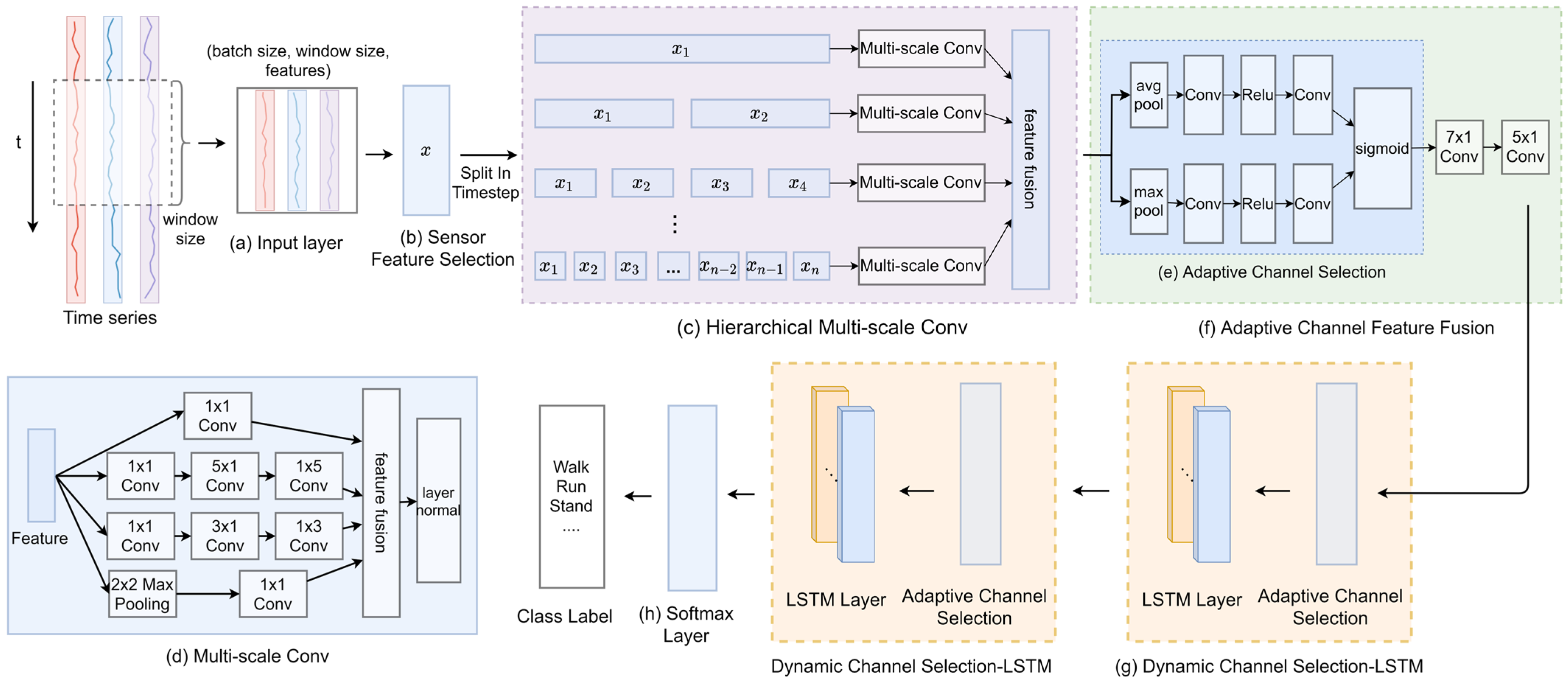
• We propose a novel HMA Conv-LSTM network, which realizes HAR that can well distinguish confusing actions of subtle processes. Extensive experiments on four public datasets of Opportunity, PAMAP2, USC-HAD, and Skoda show the effectiveness of our proposed model.
• We propose the hierarchical multi-scale convolution module, which performs finer-grained feature extraction by hierarchical architecture and multi-scale convolution on spatial information of feature vectors.
• In addition, we propose the adaptive channel feature fusion module is capable of fusing features at different scales, which improve the efficiency of the model and remove redundant information.
• For the multi-channel feature maps extracted by adaptive channel feature fusion, we propose the dynamic channel-selection-LSTM module based on the attention mechanism to extract the temporal context information.

The rest of the paper is organized as follows: Section 2 reviews previous work related to us. Section 3 details the methodology proposed in this paper. Section 4 describes the experimental setup and the four HAR benchmark datasets and compares the proposed model with state-of-the-art methods. Section 5 explores the selection of model parameters and ablation experiments, discusses the results, and analyzes the confusion matrix as well as visualizes the attention weights. Finally, Section 6 concludes the paper.

2. Related Work

Research work on sensor-based HAR can be categorized into two types: machine learning methods and deep learning methods. Earlier research works on HAR were mainly based on traditional machine learning methods such as the Random Forest (RF), Support Vector Machine (SVM), and Hidden Markov Model (HMM). Gomes et al. [31] compared the performances of three classifiers: SVM, RF, and KNN. Kasteren et al. [32] proposed a sensor that can automatically recognize actions and data labeling system; they demonstrated the performance of a HMM in recognizing actions. Tran et al. [33] constructed a HAR system via an SVM that was able to recognize six human actions by extracting 248 features. However, traditional machine learning methods rely heavily on hand-crafted features such as mean, maximum, variance, and fast Fourier transform coefficients [34]. Since extracting hand-crafted features relies on human experience and expert knowledge and only captures shallow features, the accuracy is limited.

Unlike traditional machine learning methods, deep learning can learn the feature representation of a classification task without involving domain-specific knowledge, and HAR can be achieved without extracting hand-crafted features. Yang et al. [15] proposed that CNNs can effectively capture salient features in the spatial dimension and outperform traditional machine learning methods. Jiang et al. [35] proposed a CNN model that arranges raw sensor signals into signal images as model inputs and learns low-level to high-level features from action images to achieve effective HAR.

Meanwhile, since action recognition is a time-series classification problem, it may be difficult for CNNs to capture time dimension information. In contrast, Hammerla et al. [18] and Dua et al. [19] used the LSTM network for HAR, which can effectively capture contextual information and long-term dependencies of the temporal dimension of the sensor sequence data. Ullah et al. [36] proposed a stacked LSTM network for recognizing six types of human actions using smartphone data, with 93.13% recognition accuracy. Mohsen et al. [37] used GRU to classify human actions, achieving 97% accuracy on the WISDM dataset. Gaur et al. [38] achieved a high accuracy in classifying repetitive and non-repetitive actions over time based on LSTM–RNN networks. Although the above methods can recognize some simple human actions (e.g., cycling, walking) well, the recognition of some complex actions (e.g., stair up/down, open/close door) is still challenging, which is due to the difficulty in capturing the spatio-temporal correlation of sensor signals using a single CNN or RNN network.

Recently, much of the work in HAR has focused on hybrid models of CNN and RNN. Ordóñez et al. [21] combined an CNN and an LSTM to achieve significant results in capturing spatio-temporal features from sensor signals. Yao et al. [22] constructed separate CNNs for the different types of data in the sensor inputs, and then merged them to form global feature information; they then extracted temporal relationships through an RNN to achieve HAR. Nafea et al. [39] used CNN with varying kernel dimensions and BiLSTM to capture features with different resolutions. They effectively extracted spatio-temporal features from sensor data with high accuracy.

In addition, some works address the problem that LSTMs may compress the noise of sensor data into the network. They introduce the attention mechanism to prevent the incorporation of noisy and irrelevant parts when extracting features, thus improving the effectiveness of HAR. Murahari et al. [27] added an attention layer to the DeepConvLSTM architecture proposed in Ordóñez et al. [21] to learn the correlation weight of the hidden state outputs of the LSTM layer to create context vectors, instead of directly using the last hidden state. Ma et al. [25] also proposed an architecture based on attention-enhanced CNNs and GRUs, which uses attention to augment the weight of the sensor modalities and encapsulate the temporal correlation and temporal context information of specific sensor signal features. In contrast, Mahmud et al. [26] completely discarded the recurrent structure and adapted the transformer architecture [40] proposed in the field of machine translation to use a self-attention-based neural network model to generate feature representations for classification to better recognize human actions. Zhang et al. [41] proposed a hybrid model ConvTransformer for HAR, which can fully extract local and global information of sensor signals and use attention to enhance the model feature characterization capability. Xiao et al. [42] proposed a two-stream transformer network to extract sensor features from temporal and spatial channels that effectively model the spatio-temporal dependence of sensor signals.

The attention mechanism enables the model to pay more attention to the parts that are relevant to the current recognition when processing sequence data, helping the model to capture long-term dependencies. Although these models perform well on HAR, they do not sufficiently consider fine-grained features, which may lead to the actions of some fine-grained processes being confused during classification. Therefore, we propose the HMA Conv-LSTM network for human action recognition.

3. Proposed Method

In this section, we introduce the data preprocess and explain the proposed HMA Conv-LSTM network, whose framework is shown in Figure 2.

3.1. Data Preprocess

Public datasets are usually collected by sensors under real-life conditions and may contain inconsistent, incomplete, and noisy data. To enable deep learning networks to process multidimensional sensor timing information for HAR, we perform preprocessing operations such as data complementation, normalization, and segmentation.

3.1.1. Data Completion

HAR datasets are typically acquired using inertial sensors at different body parts. The data at each sampling point are spliced according to the timestep. During the acquisition process, data may be missing at certain sampling timesteps. Although missing data at a single timestep has limited impact on the overall data, it can affect the integrity of the timing data. Therefore, linear interpolation is used to fill in missing values. Let $\left(x,y\right)$ represent missing data, where $\left(x_0,y_0\right)$ represents the previous non-missing data and $\left(x_1,y_1\right)$ represents the next non-missing data. Since the timestep $x$ is known, the missing value $y$ can be obtained by using linear interpolation:

$$y=y_0+\left(x-x_0\right)\frac{y_1-y_0}{x_1-x_0}$$

(1)

3.1.2. Data Normalization

Since different sensing unit data often use different units of measure, the range of values can vary. If raw data are used directly as input to the model, it may result in data items with large values that sway the model’s classification effect. Additionally, fluctuating unprocessed data may affect the model’s performance [43]. Therefore, we need to normalize raw data by scaling it to fall within an interval of −1 to 1. It eliminates differences in the range between different sensor channel types. Data normalization also speeds up model convergence and improves its training rate and accuracy.

For the collected dataset $D=\left\{d_1,d_2,d_3,\dots ,d_n\right\}$, each data sample contains multi-featured sensor data $d_i=\left\{x_1,x_2,\dots ,x_K\right\}$, where $K$ represents the number of features. To determine the maximum and minimum values for all features in the dataset, we form the vectors $x_{max}$ and $x_{min}$. And then, we perform the normalization operation:

$$x_i=2\times \frac{\left|x_i-x_{min}\right|}{\left|x_{max}-x_{min}\right|}-1$$

(2)

3.1.3. Data Segmentation and Downsampling

In real-life scenarios, different sampling devices and sensors have varying sampling rates. To accommodate most sensor devices, we need to downsample the data that are sampled at a higher rate. For datasets, matching the sampling rates across all data allows for a more accurate comparison of model performance on different datasets. In this case, we downsample the PAMAP2, Skoda, and USC-HAD datasets to approximately 33 Hz to match the sampling rate of the Opportunity dataset.

In this paper, our proposed model is to perform feature extraction for each action window after segmenting the sensor data sequence. The two dimensions of an action window are the timestep and the number of sensor features, respectively. Suppose the sensor data sequence is segmented using a sliding window of width $W$ and a certain overlap rate. Each window obtained can be denoted as $V=\left[v_1,\dots ,v_t,\dots ,v_W\right]$, where $v_t=\left[v_1^t,\dots ,v_K^t\right]$ represents $K$ features of the sensor at timestep $t$. In addition, the action ground truth label for each window is defined as the label with the most occurrences of each sensor data within the window. Window-wise and Sample-wise are two methods used to segment action data [26]. In our study, we uniformly use the Window-wise method on the training, validation, and test sets to ensure consistent results.

Window size and sliding window overlap rate are important factors in action recognition because different actions can vary in duration and complexity. To better evaluate and explore the impact of these factors on our model’s overall effectiveness, we deploy window size and window overlap rate as hyperparameters in our project. We specifically evaluate and explore optimal hyperparameters in Section 5.

3.2. Sensor Feature Selection

Different types of sensor features play varying roles in recognizing different actions. Using unimportant sensor features may significantly impact recognition due to noise [44]. To capture the contribution weights and potential importance of different types of sensor features, we perform the SFS operation based on the attention mechanism on the sensor input data. Not all sensor features contribute equally when performing action classification. For example, the sensor at the subject’s ankle may not contribute much when performing the “Open Drawer” action. In addition, this weight not only assigns importance to sensor input features, but also demonstrates the effectiveness of feature selection by visualizing how much attention is paid to specific features for a particular action.

The SFS operation uses a two-dimensional convolution across sensor feature values and timesteps to extract dependencies between them. First, it takes as input the sensor’s feature vectors $[v_1^t,v_2^t,\dots v_i^t,\dots ,v_K^t]$ and reshapes them into a single-channel vector, which is then processed using k convolutional filters to output a k-channel image. This is then converted back to a single channel using a $1\times 1$ convolutional kernel and the attention weights of the individual sensor feature values are obtained by the softmax operation defined in (4). The whole process can be formalized as

$$q_i^t=\tanh \left(W_1{v}_i^t+b_1\right)$$

(3)

$$s_i^t=\frac{\exp \left({\left(q_i^t\right)}^T{w}_1\right)}{{\sum }_K\exp \left({\left(q_i^t\right)}^T{w}_1\right)}$$

(4)

$$c^t={\displaystyle \sum _K}{s}_i^t{v}_i^t$$

(5)

where $i$ denotes the i-th sensor feature value, and $K$ denotes the number of features of a single timestep sensor. We first obtain the hidden representation of $v_k^t$ as $q_i^t$ from the convolutional layer, then compute the similarity between $q_i^t$ and the context vector $w_1$, and obtain the normalized attention weight $s_i^t$ by a softmax operation. $\left\{W_1,w_1,b_1\right\}$ is the trainable parameter of the attention network, and $c^t$ is the unified feature representation of all $K$ sensor features obtained after the weighted vector.

3.3. Hierarchical Multi-Scale Convolution

We proposed the HMC module to perform finer-grained feature extraction on the spatial information of the feature vectors. In the following, we will introduce the multi-scale convolution module and the entire hierarchical architecture separately.

3.3.1. Multi-Scale Convolution

In deep convolutional structures, single-size convolutional kernels often fail to provide diverse features and lack the ability to decompose on multi-scales. Since the overall process of some confusable behaviors (e.g., open/close door) is relatively similar, it is often difficult to focus on both global and local features if the network is constructed using only a single-scale convolutional kernel. Inspired by the work of Szegedy et al. [45], we use the multi-scale convolutional neural network. It utilizes convolutional kernels of different scales for multi-scale feature extraction and splicing in both sensor and temporal dimensions. This strengthens the network’s ability to recognize features of different scales, enhances its adaptability, and improves its feature characterization ability. In addition, we separate the common $N\times N$ two-dimensional convolution kernel, first convolve the temporal information by the $N\times 1$ convolution kernel, and then use the $1\times N$ convolution kernel to convolve the information of different sensor dimensions at the same timestep. The specific structure is shown in Figure 2d.

In our network structure, $1\times 1$ convolution kernels are used to organize information across channels and perform dimensionality reduction on input channels. It improves the network’s expressive power and adds a layer of features and nonlinear variations. By using convolution kernels of different sizes, we can analyze raw sensor data at multi-scales. To address the issue of vanishing and exploding gradients during network training, we perform batch normalization after weighted multi-scale feature fusion. This accelerates the network’s convergence process while keeping the distribution of test and training data the same and improving the generalization ability of the network.

3.3.2. Hierarchical Architecture

HAR relies on sequential data captured by sensors placed at various body locations, which contain spatial and temporal information about physical actions. Due to the varying durations and complexities of different actions, some actions may require longer sliding window sizes for segmentation to achieve good recognition results. However, sliding window sizes that are too large may cause the general network model to overlook some fine-grained subtle action processes, thereby affecting action recognition. In contrast, our proposed hierarchical architecture can split the action window and extract features from the sensor sequence data at a finer granularity to effectively recognize the finer action processes. The specific structure of the whole HMC module is shown in Figure 2c.

To construct the HMC network architecture, we divide the sensor feature sequence weighted by the SFS module in the time dimension, as shown in Figure 3. The HMC can capture some subtle changes of actions in human motion. By capturing the sub-actions in the sensor feature sequences, the model can obtain more detailed information, thus realizing a finer-grained HAR. In this work, we have tested experimentally and finally selected the hierarchical architecture with 2 layers of division, and the experiments show good results, as detailed in Section 5.

For the sensor feature sequence $x=\left[c^1,c^2,\dots c^i,\dots ,c^t\right]$ weighted by the SFS module, each feature vector $c_i$ consists of $\left[c_1^i,c_2^i,\dots c_j^i,\dots ,c_K^i\right]$, where $t$ denotes the number of timesteps, and $K$ denotes the number of features of a single timestep sensor. When the hierarchical number of partitions $level=0$, the sequence is not hierarchical and the feature sequence is unchanged and defaults to 1 partition, $x_1^0=x$; when the number of partitions $level=1$, the sequence is divided into 2 partitions, i.e.,

$$x_1^1=\left[c^1,c^2,\dots ,c^{\frac{t}{2}}\right],x_2^1=\left[c^{\frac{t}{2}+1},\dots ,c^{t-1},c^t\right]$$

(6)

When the number of strata $level=2$, the sequence is divided into 4 partitions, i.e.,

$$x_1^2=\left[c^1,c^2,\dots ,c^{\frac{t}{4}}\right],x_2^2=\left[c^{\frac{t}{4}+1},\dots ,c^{\frac{t}{2}}\right],x_3^2=\left[c^{\frac{t}{2}+1},\dots ,c^{\frac{3}{4}t}\right],x_4^2=\left[c^{\frac{3}{4}t+1},\dots ,c^t\right]$$

(7)

When the number of strata $level=n$, the sequence is divided into $2^n$ partitions, i.e.,

$$x_i^n=\left[c^{\frac{t\ast \left(i-1\right)}{2^n}+1},c^{\frac{t\ast \left(i-1\right)}{2^n}+2},\dots ,c^{\frac{t\ast i}{2^n}}\right],i\in \left\{1,\dots ,2^n-{1,2}^n\right\}$$

(8)

In fact, we divide the features into two each time, so the i-th sub-partition of the l-th layer comes from the $\lfloor \frac{i+1}{2}\rfloor$ parent partition of the l-1-th layer; the formulaic expression is

$$x_j^{l-1}=\left[x_{i\ast 2-1}^l,x_{i\ast 2}^l\right]$$

(9)

After the hierarchical division, all sub-partitions are presented as a pyramidal tree structure. We perform multi-scale convolutional operations on each partition of the division. We use multi-scale convolutional neural networks to extract and splice features in the sensor dimension and time dimension to strengthen the network’s ability to recognize features at different scales by multi-scale mining of the data to improve the characterization ability of the final acquired features.

Then, we first splice the multi-scale features extracted from each partitioned layer in the time dimension, and then perform feature superposition; the final features are fused to a multi-channel feature $y^{\prime }$ of the same dimension as that obtained from the original feature $x$ through the multi-scale convolutional network, which serves as the output of the whole HMC network. For layer $l$, the features can be represented as

$$y^l=concat\left(x_1^l,x_2^l,\dots ,x_{2^l}^l\right)$$

(10)

And the final fusion feature obtained is

$$y^{\prime }=y^1+y^2+\cdots +y^n$$

(11)

where $y^{\prime }$ is fused from $n$ layers of hierarchical multi-scale features. By using the Hierarchical architecture, we can capture some of the subtle changes in action during human movement. The model obtains more detailed information by acquiring sub-actions in the sequence of sensor features, thus enabling finer-grained HAR.

3.4. Adaptive Channel Feature Fusion

After acquiring the multi-scale features by HMC module, we perform ACFF operations on them. The ACS module and the multi-scale channel feature fusion operation will be described separately in the following section.

3.4.1. Adaptive Channel Selection

We proposed the ACS module to process the multi-channel feature maps, adaptively learn the weight coefficients of each channel, improve the overall model’s discriminative ability and sensitivity to each channel feature, and strengthen the channel features that are beneficial to model classification while suppressing the useless channel feature information. Its structure is shown in Figure 2e.

The ACS module mainly contains extraction operations and squeeze operations. Assume that the output vector $x$ of the multi-scale convolutional layer is of size $C\times W\times H$, where $C$ is the number of channels, and $W\times H$ denotes the size of the feature map of each channel. The extraction operation inputs $x$ into a global average pooling layer and a global maximum pooling layer to compress the features, resulting in channel-level statistical information $Z_{avg}$ and $Z_{max}$. This information encodes the spatial features on each channel as a real number with a global receptive field representing the global features of the feature maps. The output dimensions match the number of feature channels input. The formulas for finding $Z_c^{avg}$ and $Z_c^{max}$ for each channel are as follows:

$$Z_c^{avg}=\frac{1}{W\times H}{\displaystyle \sum _{i=1}^W}{\displaystyle \sum _{j=1}^H}{x}_c\left(i,j\right)$$

(12)

$$Z_c^{max}={\displaystyle \underset{1\le i\le W}{\max }}{\displaystyle \underset{1\le j\le H}{\max }}{x}_c(i,j)$$

(13)

where $x_c\left(i,j\right)$ represents the value of row $i$ and column $j$ in the c-channel feature map. After the extraction operation, the global description features are obtained for each channel. And the activation operation aims to obtain the relationship between the channels, which is achieved by using two fully connected layers. The first fully connected layer plays the role of dimensionality reduction, downgrading the channel dimensions of $Z_c^{avg}$ and $Z_c^{max}$ to 1/16 of their original dimensions to change the capacity and computational cost of the ACS module in the network. It is then activated by the ReLU function and upscaled to the original channel dimensions using a second fully connected layer. Finally, the normalized weights are obtained using the Sigmoid activation function after superimposing the channel dimensions computed by the two branches of global average pooling and global maximum pooling. The formula for the activation operation is expressed as

$$s=Sigmoid\left(W_1·ReLU\left(W_0·Z_{avg}\right)+W_1·ReLU\left(W_0·Z_{max}\right)\right)$$

(14)

where $W_0\in R^{\frac{C}{16}\times C}$ and $W_1\in R^{C\times \frac{C}{16}}$; finally, the learned weights $s_c$ for each channel are multiplied by the original individual channel features $x_c$:

$$y_c=s_c\times x_c$$

(15)

The output dimensions of the extraction and squeeze operations of the ACS module are unchanged, and the whole process can be viewed as learning the weight coefficients of each channel adaptively to improve the overall model’s discriminative ability and sensitivity to the features of each channel.

3.4.2. Multi-Scale Channel Feature Fusion

We propose the ACFF module to process the acquired multi-scale feature maps. The module consists of an ACS module and two convolutional layers. Its structure is shown in Figure 2f. Using different sizes of convolutional kernels can extract features at different scales. Here, we use a convolutional layer containing 64 convolutional kernels of sizes $7\times 1$ and $5\times 1$ to extract local time-domain features and ultimately achieve ACFF at different scales. For the multi-channel feature map $x_1$, assuming the size of $C\times W\times H$, the whole process is formulaically expressed as

$$f_1\left(x_1\right)={\displaystyle \sum _{c=1}^C}{\displaystyle \sum _{r=1}^7}{x}_1\left(c,i,j+r-1\right)W_1\left(c,k,r\right)$$

(16)

$$f_2\left(x_2\right)={\displaystyle \sum _{c=1}^{64}}{\displaystyle \sum _{r=1}^5}{x}_2\left(c,i,j+r-1\right)W_2(c,k,r)$$

(17)

$$y=f_2\left(f_1\left(x_1\right)\right)$$

(18)

where $W_1$ and $W_2$ denote the convolution kernels of the two convolutional layers, respectively, and $x_1\left(c,i,j\right)$ denotes the value of input $x_1$ in the c-th channel of row $i$ and column $j$. $r$ denotes the convolution width. $k$ denotes the number of convolution kernels, which is the number of output channels of the convolutional layer. Finally, after two convolution layers, the output feature is $y$.

In conclusion, the ACFF module performs multi-scale feature extraction and fusion of multi-channel feature maps. It can reduce the amount of computation while retaining important spatial information. Moreover, it can improve the efficiency and interpretability of the model, remove redundant information, and realize the fusion of features at different scales.

3.5. Dynamic Channel-Selection-LSTM

For the channel feature maps obtained after ACFF, to establish the connection between different timestep feature vectors, we use two proposed DCS-LSTM modules to extract the temporal context information of the sensor signals, the structure of which is shown in Figure 2g. In addition, Karpathy et al. [46] pointed out that models containing at least two recurrent layers work better in processing sequence data. Here, we similarly use the ACS operation to obtain the contributions of different channels, adaptively learn the weight coefficients of each channel, and strengthen the ability to characterize features for the classification of confusable behaviors. The structure of the basic LSTM network cell is shown in Figure 4.

The forgetting gate decides what information to let continue through that neuron. The input gate decides how much information to update to the state matrix. The output gate combines the neuron’s state vectors, the input vectors, and the output vectors of the previous neuron to arrive at the output value for the current moment. Its vector update operation is represented as

$$i_t=\sigma \left(W_{ai}{a}_t+W_{hi}{h}_{t-1}+W_{ci}{c}_{t-1}+b_i\right)$$

(19)

$$f_t=\sigma \left(W_{af}{a}_t+W_{hf}{h}_{t-1}+W_{cf}{c}_{t-1}+b_f\right)$$

(20)

$$o_t=\sigma \left(W_{ao}{a}_t+W_{ho}{h}_{t-1}+W_{co}{c}_t+b_o\right)$$

(21)

$$c_t=f_t{c}_{t-1}+i_t\sigma \left(W_{ac}{a}_t+W_{hc}{h}_{t-1}+b_c\right)$$

(22)

$$h_t=o_t\sigma \left(c_t\right)$$

(23)

where $i_t$, $f_t$, and $o_t$ are the output vectors of the input, forgetting, and output gates of the LSTM cell at time $t$, respectively; $c_t$ is the state vector of the LSTM cell at time $t$; $\mathsf{\sigma }$ is a sigmoid nonlinear excitation function that introduces a nonlinear factor; $a_t$ is the input vector of the LSTM cell at time $t$; $W$ stands for the weight matrix for the connection between different gates; and $b$ is the bias vector.

LSTM can record the feature representation of longer sequence data. Therefore, we proposed the DCS-LSTM network to implement the time-series modeling work on the data to facilitate the extraction of temporal contextual information of the sensor signals and weight the channel features by an ACS module to improve the model’s ability to discriminate individual channel features and classify confusable behaviors. The hidden cells of the LSTM are set to 128.

4. Experiments

In this section, we conduct comprehensive experiments on several public HAR datasets to validate the effectiveness of our proposed framework. First, we describe the experimental setup, training measures, and evaluation metrics. Then, we present the benchmark datasets used. Finally, we compare our proposed model with state-of-the-art methods from recent years and report on the performance of HMA Conv-LSTM.

4.1. Experimental Setup

We build the model using Google’s open-source deep learning framework TensorFlow 2.9.0, implement it using Python 3.8, and train it on an Intel Xeon Platinum 8255C CPU and an RTX 3080 GPU with 10 GB of memory. In addition, we used the Adam optimizer [47] to minimize the cross-entropy loss function for model training. The learning rate adopts Adam’s default parameter of 0.001 as the initial training parameter of the model. We also use a cosine learning rate scheduling strategy to dynamically adjust the learning rate according to the cosine function in each epoch. The batch size of the four datasets is set to 128, and the number of training epochs is 80. Details of the hyperparameters used for model training are shown in

Table 1. Hyperparameters of the model trained.

Hyperparameters	Value
Optimizer	Adam
Loss function	Cross entropy
Batch size	128
Learning rate	0.001
Learning rate scheduler	Cosine
Training epoch	80
Dropout rate	0.3

.

4.2. Dataset Description

We conducted experiments on the proposed HMA Conv-LSTM model on four benchmark datasets [48] with the same experimental setup as in the previous work.

Table 2. Summary of the datasets. Here A = Accelerometer, G = Gyroscope, M = Magnetometer.

Dataset	Action Number	Validation Subject ID	Test Subject ID	Sampling Rate	Downsampling	Sensors Used
Opportunity	18	1(Run 2)	2, 3(Run 4, 5)	30 Hz	100%	A, G, M
PAMAP2	12	105	106	100 Hz	33%	A, G
USC-HAD	12	11, 12	13, 14	100 Hz	33%	A, G
Skoda	11	1(10%)	1(10%)	98 Hz	33%	A

shows the basic information statistics of the four datasets. Figure 5 shows the distribution of sample categories for the four benchmark datasets.

Opportunity dataset [49] mainly contains daily household and kitchen actions. Subjects recorded data using inertial measurement units (IMUs) such as accelerometers, gyroscopes, and magnetometers at 12 locations on the body. The dataset is annotated for 18 mid-level actions (e.g., opening/closing the refrigerator), with one null category exceeding 76% of the data. It makes the dataset highly unbalanced in terms of the distribution of action categories.

PAMAP2 dataset [50] mainly contains multiple household actions. A total of nine subjects were instructed to perform 12 actions of daily living. Subjects recorded complete IMU data, temperature, and heart rate data using three wearable sensors located on the hand, chest, and ankle.

USC-HAD dataset [51] includes six readings from three-axis accelerometers and gyroscopes worn on the subjects’ bodies. It contains 12 different action categories from 14 subjects, including walking, running, elevator up/down, etc. In addition, the sensor locations and division of action categories in this dataset make classification using feature representation learning challenging. For example, it is difficult to discriminate between actions such as walking to the left or right using only accelerometers and gyroscopes.

Skoda dataset [52] mainly consists of 10 actions performed by workers in an automotive production environment, such as opening/closing doors and check steering wheel. It also includes labeled empty categories. It consisted of one subject wearing an accelerometer in several different positions on their arm to perform manual maintenance and quality checks on automotive parts.

4.3. Performance Metric

In our experiments, we use the Macro average F1-score as the evaluation metric to compare the performance of our proposed method with other methods. In particular, for the Opportunity dataset, accuracy is not a suitable measure due to its highly uneven categorization. Since the traditional F1-score measures the performance of binary classification, we use the mean F1-score, which is $F_m$, weighted to categories according to their sample proportions.

$$F_m=\frac{1}{C}{\displaystyle \sum _{i=1}^C}\frac{2\times Precisio{n}_i\times Recal{l}_i}{Precisio{n}_i+Recal{l}_i}$$

(24)

where $C$ is the number of action categories. For category $i$, $Precisio{n}_i=\frac{T{P}_i}{T{P}_i + F{P}_i}$, $Recal{l}_i=\frac{T{P}_i}{T{P}_i + F{N}_i}$. $T{P}_i$ and $F{P}_i$ are the number of true positives and false positives, respectively, while $F{N}_i$ refers to the number of false negatives.

4.4. Comparison with State-of-the-Art Methods

In this section, we compare our proposed model with related work from recent years. The selected baseline approach is based on the four public datasets in Table 2. Firstly, our model outperforms SVM because earlier machine learning methods relied heavily on hand-crafted features, which limited their accuracy. Additionally, our model outperforms CNN and LSTM, which only consider either temporal contextual relevance or spatial relevance. Secondly, our model is more accurate than the DeepConvLSTM and DeepConvLSTM + Attention models because our HMC structure effectively captures finer-grained information about tiny action processes. Furthermore, our model is more accurate than recently proposed methods such as ConvAE, AttnSense, and Self-Attention that incorporate attention mechanism. It reflects that our model outperforms most existing models and illustrates the effectiveness of our hierarchical architecture for feature extraction. In addition,

Table 3. Macro F1-score of different methods on the benchmark set.

Methods	Opportunity	PAMAP2	USC-HAD	Skoda
SVM [53]	-	0.71	-	0.82
RF [54]	-	0.74	-	0.83
CNN [55]	0.59	0.82	0.41	0.85
LSTM [56]	0.63	0.75	0.38	0.89
b-LSTM [18]	0.68	0.84	0.39	0.91
DeepConvLSTM [21]	0.67	0.75	0.38	0.91
DeepConvLSTM + Attention [27]	0.71	0.88	-	0.91
LSTM + Continuous Attention [57]	-	0.90	-	0.94
ConvAE [48]	0.72	0.80	0.46	0.79
SADeepSense [58]	0.66	0.66	0.49	0.90
AttnSense [25]	0.66	0.89	0.49	0.93
Self-Attention * [26]	0.63	0.84	0.51	0.87
HMA Conv-LSTM	0.68	0.91	0.53	0.96

Models with * indicate that the performance is obtained by our replication. The bold parts represent our proposed model and the best performance on each dataset.

is categorized by network type, which are traditional models, LSTM-based, and attention mechanism-based models, and, finally, our proposed model.

As shown in Table 3, the recognition performance of HMA Conv-LSTM significantly outperforms the other baselines. Despite USC-HAD being a challenging dataset, our model performs better than other models such as DeepConvLSTM (0.38) and AttnSense (0.49). Additionally, our proposed model outperforms other models which are based on attention mechanisms. On the PAMAP2 dataset, our model achieves better results (0.91) than DeepCovnLSTM + Attention (0.88), LSTM + Continuous Attention (0.90), and AttnSense (0.89). For the Skoda dataset, our model achieves high performance and outperforms other well-performing models such as AttnSense (0.93) and LSTM + Continuous Attention (0.94). In addition, compared to other methods, our model performs well on the Opportunity dataset (0.68), which contains complex actions. Due to the short duration of some of these mid-level gestures, the hierarchical architecture does not improve the current results much. However, when considering more complex and confusing gestures, the effect of our model is evident.

In conclusion, our proposed model outperforms other baseline methods on all datasets except the Opportunity dataset. It demonstrates the effectiveness and contribution of our model. The evaluation results further show that our proposed HMA Conv-LSTM can effectively obtain both temporal context information and spatial information from sensor sequence data. It can also recognize some subtle action processes with fine-grained detail, ultimately achieving good results.

5. Ablation Study and Discussion

We evaluate the effectiveness of our proposed HMA Conv-LSTM model. First, we explored the effect of the choice of model hyperparameters on performance. Second, we evaluated the effectiveness and contribution of each module of the model through ablation experiments. Then, we analyzed the confusion matrix obtained by testing the model on some of these datasets. Finally, we visualized the feature weights in SFS when recognizing some actions to improve the interpretability of the model.

5.1. Parameter Selection

To evaluate the impact of hyperparameters on the model’s overall performance, we explored the sliding window size, sliding window overlap rate, and the number of hierarchical layers. We adjusted them sequentially and finally chose the optimal parameters. First, we analyzed the effect of sliding window size on the model’s recognition performance. The four datasets were previously downsampled uniformly to a sampling rate of about 33 Hz per second. Since the repetition period of different actions varies, we experimented by changing the window size in seconds.

In Figure 6, our proposed model is more stable to changes in window size compared to other models. It also indicates that some complex actions require longer sliding window sizes for segmentation to achieve good recognition results. When the initial window size is small, the performance is average because the HMC structure has difficulty capturing information on multi-scales. As the window size increases, the model’s performance improves, demonstrating the effectiveness of the hierarchical architecture and multi-scale convolution for feature extraction at different scales. The DCS-LSTM can also better capture temporal context information. Considering the performance, we chose a sliding window size of 1 s for the PAMAP2 and USC-HAD datasets, while the Opportunity and SKODA datasets chose a sliding window size of 1.5 s for action recognition.

Then, based on the optimal sliding window size, we also discussed the impact of sliding window overlap rate on model performance. Due to the varying durations and complexities of different actions, the sliding window overlap rate is also critical in affecting action recognition. In Figure 7a, the model’s performance on most datasets increases as the window overlap rate starts to increase, and the model reaches its best result when the overlap rate reaches 0.5. As the overlap rate continues to increase, the model’s performance starts to decrease. This suggests that an appropriate overlap ratio can help the model better capture local patterns and relationships in time series data, maximizing the information in the data while ensuring computational efficiency. Therefore, we chose 50% as the window overlap rate for model training. Finally, based on the optimal configuration, we explored the number of layers in the hierarchical architecture of our proposed model.

In Figure 7b, as the number of layers increases from zero to two, the model’s performance improves on each dataset. This indicates that our proposed HMA Conv-LSTM network can effectively capture multi-scale features and some fine-grained subtle action processes. However, when the number of layers reaches three, the performance starts to deteriorate. The window size may be the cause of this situation. When the number of layers is three, the minimum division of the partition length is small, and the multi-scale convolution operation can no longer capture finer features. The model’s best results are obtained when the number of layers is two. Therefore, we choose two as the number of hierarchical layers for model construction.

5.2. Effectiveness of the Proposed Modules

We conducted an ablation study on the proposed model, based on the optimal parameter configurations of the previous model, to evaluate the contributions of the proposed modules. The results of the ablation experiments are shown in

Table 4. Ablation study results compared with the full HMA Conv-LSTM model (Macro F1-score).

Model	Opportunity		PAMAP2		USC-HAD		Skoda
	F1-Score	∆	F1-Score	∆	F1-Score	∆	F1-Score	∆
HMA Conv-LSTM	0.68	-	0.91	-	0.53	-	0.96	-
-SFS	0.65	−0.03	0.87	−0.04	0.51	−0.02	0.93	−0.03
-ACFF (+Two Convolution Layer)	0.65	−0.03	0.89	−0.02	0.50	−0.03	0.94	−0.02
-DCS-LSTM (+LSTM)	0.66	−0.02	0.89	−0.02	0.51	−0.02	0.93	−0.03
-HMC	0.61	−0.07	0.86	−0.05	0.48	−0.05	0.91	−0.05
-HMC (+Multi-scale Convolution)	0.64	−0.04	0.87	−0.04	0.50	−0.03	0.93	−0.03

The bold parts represent the performance of our proposed model before ablation on each dataset.

. In each experiment, we removed specific modules from the proposed model. Additionally, we replaced the ablated modules with alternative modules in some experiments for further testing. For example, we replaced the entire HMC with multi-scale convolution and replaced DCS-LSTM with LSTM. We also deleted ACS in ACFF and used the remaining two convolutional layers instead.

From Table 4, it is evident that HMC significantly contributes to improving recognition. Its ablation leads to about 0.05 performance degradation across datasets. While the ablation of SFS leads to about 0.03 performance degradation. When we replaced the HMC component with a single multi-scale convolution component, the model performance also decreased by about 0.03, illustrating the importance and effectiveness of the hierarchical architecture and suggesting that multi-scale feature maps captured by the multi-scale convolution are effective.

Regarding DCS-LSTM, replacing it with a standard LSTM network resulted in a performance decrease of about 0.02, indicating that the ACS operation effectively captures contributions from different channels and learns each channel’s weights adaptively. When ACS was ablated from the ACFF component, performance decreased by about 0.02, further demonstrating ACS operation’s effectiveness. In conclusion, all components in our proposed model significantly contribute to its performance, as evidenced by the results of our ablation experiments. In addition, our study also has some limitations. Our model depends on the quality of the sensor signal. If there are a lot of noise or data missing, it may affect the model’s performance.

5.3. Comparison of Specific Actions

Figure 8 and Figure 9 shows the confusion matrix of our proposed model on the PAMAP2, USC-HAD, Skoda, and Opportunity datasets. The confusion matrix is used to measure the effectiveness of a classifier in recognizing different categories. The row and column labels of a confusion matrix represent the true and predicted categories, respectively. The diagonal elements of the confusion matrix indicate the correct recognition rate for each action, while the off-diagonal elements represent the proportion of actions that are incorrectly recognized as other categories.

In Figure 8a, there is some confusion between “standing” and “sitting”, which is reasonable because the two actions are relatively similar. Other categories such as “walking”, “running”, and “descending stairs” are well recognized. In Figure 8b, there is some confusion about the type of action due to the division of the sensor’s position and action category at the time of data acquisition. However, for some categories such as “Walking Forward”, “Walking Right”, “Walking Upstairs”, etc., our model is still able to distinguish the confusing actions well.

In Figure 9a, there is some confusion between the actions “open left front door” and “close left front door” due to the similarity of the two actions, resulting in similar data collected by the accelerometer. However, other action categories, such as “open hood”, “close hood”, and “close both left doors” were well recognized. This is because these actions are process-oriented and can be distinguished without serious confusion, and the model is more sensitive to the data collected by the sensors. In Figure 9b, human action recognition on the Opportunity dataset is challenging due to the highly unbalanced sample distribution. Nevertheless, our model can still distinguish some easily confused actions, such as “Open Door 1” and “Open Door 2”, “Close Door 1” and “Close Door 2”, “Open Drawer 3” and “Close Drawer 3”, etc. This shows that our proposed model can effectively and accurately recognize some complex actions with subtle processes and can also distinguish some confusing actions well.

In addition, the evaluation metrics scores for each category on the Skoda and Opportunity datasets are presented in

Table 5. Evaluation metrics for each action of the proposed model on the Skoda dataset.

Action of Skoda Dataset	Precision	Recall	Macro F1-Score
null	0.996	0.999	0.998
write on notepad	0.989	0.988	0.989
open hood	0.980	0.955	0.968
close hood	0.959	0.983	0.970
check gaps on the front door	0.989	0.989	0.989
open left front door	0.834	0.903	0.867
close left front door	0.890	0.809	0.848
close both left door	0.987	0.991	0.989
check trunk gaps	0.989	0.988	0.988
open and close trunk	0.988	0.991	0.989
check steering wheel	0.999	0.980	0.990

and

Table 6. Evaluation metrics for each action of the proposed model on the Opportunity dataset.

Action of Opportunity Dataset	Precision	Recall	Macro F1-Score
Other	0.949	0.964	0.956
Open Door 1	0.842	0.800	0.821
Open Door 2	0.844	0.750	0.794
Close Door 1	0.944	0.739	0.829
Close Door 2	0.750	0.938	0.833
Open Fridge	0.800	0.675	0.732
Close Fridge	0.733	0.746	0.740
Open Dishwasher	0.595	0.658	0.625
Close Dishwasher	0.486	0.586	0.531
Open Drawer 1	0.294	0.385	0.333
Close Drawer 1	0.539	0.467	0.500
Open Drawer 2	0.889	0.500	0.640
Close Drawer 2	0.636	0.700	0.667
Open Drawer 3	0.606	0.769	0.678
Close Drawer 3	0.560	0.667	0.609
Clean Table	0.909	0.526	0.667
Drink from Cup	0.762	0.647	0.700
Toggle Switch	0.857	0.450	0.590

, respectively. The main focus here is to analyze the performance of the Macro F1-score. In Table 5, the “close left front door” action has the lowest Macro F1-score of 0.85; while the actions such as “write on notepad” and “check steering wheel” have a higher Macro F1-score of 0.99. In Table 6, the Macro F1-score performance of confusing actions such as “Open Door 1”, “Open Door 2”, “Close Door 1”, and “Close Door 2” all reached above 0.79, while the Macro F1-score performance of “Open Drawer 2”, “Close Drawer 2”, “Open Drawer 3”, and “Close Drawer 3” also reached above 0.6, which is generally a good performance. These results indicate that our proposed model has good action recognition performance.

5.4. Visualizing Sensor Feature Selection Weights

We visualized the attentional weights in the SFS module to evaluate the effects of different sensor features on different parts of the human body and different actions. Figure 10a shows the IMU inertial sensing units in different parts of the human body in the PAMAP2 dataset; Figure 10b,c shows the attentional weights of the different sensor features for the actions of “running” and “ironing”, respectively.

In Figure 10b, the “hand_acc”, “chest_acc”, and “ankle_acc” three-axis sensors in the IMU have a significant impact on the running action. This is reasonable and intuitively understandable because all parts of the human body are coordinated to complete actions during running, and different types of sensor features play different roles in recognizing different actions. In Figure 10c, the “hand_acc” sensor in the IMU is given more weight, which is also reasonable because ironing is mainly performed with the hand.

Not all sensor features have the same contribution when performing action classification. Our SFS module can automatically learn the weights of different sensor features in the HAR task, capturing their contributions and potential importance. In short, our module effectively identifies sensor features that contribute to the HAR task, providing a more accurate basis for action classification.

6. Conclusions

In this paper, we proposed the HMA Conv-LSTM, a novel hierarchical multi-scale adaptive Conv-LSTM network for HAR. This network attentively weights sensor signals by SFS, extracts finer-grained spatial features using HMC, and employs ACFF to process multi-channel feature maps. It extracts temporal context information through a DCS-LSTM network. The model fuses spatial features at different scales with time series information at different levels to effectively capture the spatio-temporal motion patterns of the sensor signals and accurately recognize some actions with fine-grained processes. Extensive experiments on four public datasets demonstrate that HMA Conv-LSTM achieves competitive performance when compared to several state-of-the-art approaches.

In future work, we will continue to improve our model by experimenting with new network structures and techniques to improve the performance of the model. We will also consider using some data noise reduction and data augmentation operations to improve the data quality, reduce the impact of noise on the model performance, and improve the model’s generalization ability.

References

1. Anagnostis, A.; Benos, L.; Tsaopoulos, D.; Tagarakis, A.; Tsolakis, N.; Bochtis, D. Human activity recognition through recurrent neural networks for human–robot interaction in agriculture. Appl. Sci. 2021, 11, 2188. [Google Scholar] [CrossRef]
2. Asghari, P.; Soleimani, E.; Nazerfard, E. Online human activity recognition employing hierarchical hidden Markov models. J. Ambient Intell. Humaniz. Comput. 2020, 11, 1141–1152. [Google Scholar] [CrossRef]
3. Ramos, R.G.; Domingo, J.D.; Zalama, E.; Gómez-García-Bermejo, J.; López, J. SDHAR-HOME: A sensor dataset for human activity recognition at home. Sensors 2022, 22, 8109. [Google Scholar] [CrossRef] [PubMed]
4. Khan, W.Z.; Xiang, Y.; Aalsalem, M.Y.; Arshad, Q. Mobile phone sensing systems: A survey. IEEE Commun. Surv. Tutor. 2012, 15, 402–427. [Google Scholar] [CrossRef]
5. Taylor, K.; Abdulla, U.A.; Helmer, R.J.; Lee, J.; Blanchonette, I. Activity classification with smart phones for sports activities. Procedia Eng. 2011, 13, 428–433. [Google Scholar] [CrossRef]
6. Zhang, S.; Wei, Z.; Nie, J.; Huang, L.; Wang, S.; Li, Z. A review on human activity recognition using vision-based method. J. Healthc. Eng. 2017, 2017, 3090343. [Google Scholar] [CrossRef]
7. Dang, L.M.; Min, K.; Wang, H.; Piran, M.J.; Lee, C.H.; Moon, H. Sensor-based and vision-based human activity recognition: A comprehensive survey. Pattern Recognit. 2020, 108, 107561. [Google Scholar] [CrossRef]
8. Abdel-Salam, R.; Mostafa, R.; Hadhood, M. Human activity recognition using wearable sensors: Review, challenges, evaluation benchmark. In Proceedings of the International Workshop on Deep Learning for Human Activity Recognition, Montreal, QC, Canada, 21–26 August 2021; pp. 1–15. [Google Scholar]
9. Sun, Z.; Ke, Q.; Rahmani, H.; Bennamoun, M.; Wang, G.; Liu, J. Human action recognition from various data modalities: A review. IEEE Trans. Pattern Anal. Mach. Intell. 2022, 45, 3200–3225. [Google Scholar] [CrossRef]
10. Bulling, A.; Blanke, U.; Schiele, B. A tutorial on human activity recognition using body-worn inertial sensors. ACM Comput. Surv. (CSUR) 2014, 46, 1–33. [Google Scholar] [CrossRef]
11. Bao, L.; Intille, S.S. Activity recognition from user-annotated acceleration data. In Proceedings of the International Conference on Pervasive Computing, Nottingham, UK, 7–10 September 2004; pp. 1–17. [Google Scholar]
12. Plötz, T.; Hammerla, N.Y.; Olivier, P.L. Feature learning for activity recognition in ubiquitous computing. In Proceedings of the Twenty-Second International Joint Conference on Artificial Intelligence, Barcelona, Spain, 16–22 July 2011. [Google Scholar]
13. Bengio, Y. Deep learning of representations: Looking forward. In Proceedings of the Statistical Language and Speech Processing, Tarragona, Spain, 29–31 July 2013; pp. 1–37. [Google Scholar]
14. Islam, M.M.; Nooruddin, S.; Karray, F.; Muhammad, G. Human activity recognition using tools of convolutional neural networks: A state of the art review, data sets, challenges, and future prospects. Comput. Biol. Med. 2022, 149, 106060. [Google Scholar] [CrossRef]
15. Yang, J.; Nguyen, M.N.; San, P.P.; Li, X.; Krishnaswamy, S. Deep convolutional neural networks on multichannel time series for human activity recognition. In Proceedings of the Twenty-Fourth International Joint Conference on Artificial Intelligence, Buenos Aires, Argentina, 25–31 July 2015; pp. 3995–4001. [Google Scholar]
16. Ha, S.; Yun, J.-M.; Choi, S. Multi-modal convolutional neural networks for activity recognition. In Proceedings of the 2015 IEEE International Conference on Systems, Man, and Cybernetics, Hong Kong, China, 9–12 October 2015; pp. 3017–3022. [Google Scholar]
17. Guan, Y.; Plötz, T. Ensembles of deep lstm learners for activity recognition using wearables. Proc. ACM Interact. Mob. Wearable Ubiquitous Technol. 2017, 1, 1–28. [Google Scholar] [CrossRef]
18. Hammerla, N.Y.; Halloran, S.; Plötz, T. Deep, convolutional, and recurrent models for human activity recognition using wearables. arXiv 2016, arXiv:1604.08880. [Google Scholar]
19. Dua, N.; Singh, S.N.; Semwal, V.B. Multi-input CNN-GRU based human activity recognition using wearable sensors. Computing 2021, 103, 1461–1478. [Google Scholar] [CrossRef]
20. Zhao, Y.; Yang, R.; Chevalier, G.; Xu, X.; Zhang, Z. Deep residual bidir-LSTM for human activity recognition using wearable sensors. Math. Probl. Eng. 2018, 2018, 7316954. [Google Scholar] [CrossRef]
21. Ordóñez, F.J.; Roggen, D. Deep convolutional and lstm recurrent neural networks for multimodal wearable activity recognition. Sensors 2016, 16, 115. [Google Scholar] [CrossRef]
22. Yao, S.; Hu, S.; Zhao, Y.; Zhang, A.; Abdelzaher, T. Deepsense: A unified deep learning framework for time-series mobile sensing data processing. In Proceedings of the 26th International Conference on World Wide Web, Perth, Australia, 3–7 April 2017; pp. 351–360. [Google Scholar]
23. Nan, Y.; Lovell, N.H.; Redmond, S.J.; Wang, K.; Delbaere, K.; van Schooten, K.S. Deep learning for activity recognition in older people using a pocket-worn smartphone. Sensors 2020, 20, 7195. [Google Scholar] [CrossRef]
24. Radu, V.; Tong, C.; Bhattacharya, S.; Lane, N.D.; Mascolo, C.; Marina, M.K.; Kawsar, F. Multimodal deep learning for activity and context recognition. Proc. ACM Interact. Mob. Wearable Ubiquitous Technol. 2018, 1, 1–27. [Google Scholar] [CrossRef]
25. Ma, H.; Li, W.; Zhang, X.; Gao, S.; Lu, S. AttnSense: Multi-level attention mechanism for multimodal human activity recognition. In Proceedings of the International Joint Conference on Artificial Intelligence, Macao, China, 10–16 August 2019; pp. 3109–3115. [Google Scholar]
26. Mahmud, S.; Tonmoy, M.; Bhaumik, K.K.; Rahman, A.M.; Amin, M.A.; Shoyaib, M.; Khan, M.A.H.; Ali, A.A. Human activity recognition from wearable sensor data using self-attention. arXiv 2020, arXiv:2003.09018. [Google Scholar]
27. Murahari, V.S.; Plötz, T. On attention models for human activity recognition. In Proceedings of the 2018 ACM International Symposium on Wearable Computers, Singapore, 8–12 October 2018; pp. 100–103. [Google Scholar]
28. Haque, M.N.; Tonmoy, M.T.H.; Mahmud, S.; Ali, A.A.; Khan, M.A.H.; Shoyaib, M. Gru-based attention mechanism for human activity recognition. In Proceedings of the 2019 1st International Conference on Advances in Science, Engineering and Robotics Technology (ICASERT), Dhaka, Bangladesh, 3–5 May 2019; pp. 1–6. [Google Scholar]
29. Al-qaness, M.A.; Dahou, A.; Abd Elaziz, M.; Helmi, A. Multi-ResAtt: Multilevel residual network with attention for human activity recognition using wearable sensors. IEEE Trans. Ind. Inform. 2022, 19, 144–152. [Google Scholar] [CrossRef]
30. Duan, F.; Zhu, T.; Wang, J.; Chen, L.; Ning, H.; Wan, Y. A Multi-Task Deep Learning Approach for Sensor-based Human Activity Recognition and Segmentation. IEEE Trans. Instrum. Meas. 2023, 72, 2514012. [Google Scholar] [CrossRef]
31. Gomes, E.; Bertini, L.; Campos, W.R.; Sobral, A.P.; Mocaiber, I.; Copetti, A. Machine learning algorithms for activity-intensity recognition using accelerometer data. Sensors 2021, 21, 1214. [Google Scholar] [CrossRef] [PubMed]
32. Van Kasteren, T.; Noulas, A.; Englebienne, G.; Kröse, B. Accurate activity recognition in a home setting. In Proceedings of the 10th International Conference on Ubiquitous Computing, Seoul, Republic of Korea, 21–24 September 2008; pp. 1–9. [Google Scholar]
33. Tran, D.N.; Phan, D.D. Human activities recognition in android smartphone using support vector machine. In Proceedings of the 2016 7th International Conference on Intelligent Systems, Modelling and Simulation (Isms), Bangkok, Thailand, 25–27 January 2016; pp. 64–68. [Google Scholar]
34. Figo, D.; Diniz, P.C.; Ferreira, D.R.; Cardoso, J.M. Preprocessing techniques for context recognition from accelerometer data. Pers. Ubiquitous Comput. 2010, 14, 645–662. [Google Scholar] [CrossRef]
35. Jiang, W.; Yin, Z. Human activity recognition using wearable sensors by deep convolutional neural networks. In Proceedings of the 23rd ACM International Conference on Multimedia, Brisbane, Australia, 26–30 October 2015; pp. 1307–1310. [Google Scholar]
36. Ullah, M.; Ullah, H.; Khan, S.D.; Cheikh, F.A. Stacked lstm network for human activity recognition using smartphone data. In Proceedings of the 8th European Workshop on Visual Information Processing (EUVIP), Roma, Italy, 28–31 October 2019; pp. 175–180. [Google Scholar]
37. Mohsen, S. Recognition of human activity using GRU deep learning algorithm. Multimed. Tools Appl. 2023, 1–17. [Google Scholar] [CrossRef]
38. Gaur, D.; Kumar Dubey, S. Development of Activity Recognition Model using LSTM-RNN Deep Learning Algorithm. J. Inf. Organ. Sci. 2022, 46, 277–291. [Google Scholar]
39. Nafea, O.; Abdul, W.; Muhammad, G.; Alsulaiman, M. Sensor-based human activity recognition with spatio-temporal deep learning. Sensors 2021, 21, 2141. [Google Scholar] [CrossRef]
40. Vaswani, A.; Shazeer, N.; Parmar, N.; Uszkoreit, J.; Jones, L.; Gomez, A.N.; Kaiser, Ł.; Polosukhin, I. Attention is all you need. arXiv 2017, arXiv:1706.03762. [Google Scholar]
41. Zhang, Z.; Wang, W.; An, A.; Qin, Y.; Yang, F. A human activity recognition method using wearable sensors based on convtransformer model. Evol. Syst. 2023, 1–17. [Google Scholar] [CrossRef]
42. Xiao, S.; Wang, S.; Huang, Z.; Wang, Y.; Jiang, H. Two-stream transformer network for sensor-based human activity recognition. Neurocomputing 2022, 512, 253–268. [Google Scholar] [CrossRef]
43. Zhao, C.; Huang, X.; Li, Y.; Yousaf Iqbal, M. A double-channel hybrid deep neural network based on CNN and BiLSTM for remaining useful life prediction. Sensors 2020, 20, 7109. [Google Scholar] [CrossRef]
44. Zeng, M.; Wang, X.; Nguyen, L.T.; Wu, P.; Mengshoel, O.J.; Zhang, J. Adaptive activity recognition with dynamic heterogeneous sensor fusion. In Proceedings of the 6th International Conference on Mobile Computing, Applications and Services, Austin, TX, USA, 6–7 November 2014; pp. 189–196. [Google Scholar]
45. Szegedy, C.; Liu, W.; Jia, Y.; Sermanet, P.; Reed, S.; Anguelov, D.; Erhan, D.; Vanhoucke, V.; Rabinovich, A. Going deeper with convolutions. In Proceedings of the IEEE Conference on Computer Vision and Pattern Recognition, Boston, MA, USA, 7–12 June 2015; pp. 1–9. [Google Scholar]
46. Karpathy, A.; Johnson, J.; Fei-Fei, L. Visualizing and understanding recurrent networks. arXiv 2015, arXiv:1506.02078. [Google Scholar]
47. Kingma, D.P.; Ba, J. Adam: A method for stochastic optimization. arXiv 2014, arXiv:1412.6980. [Google Scholar]
48. Haresamudram, H.; Anderson, D.V.; Plötz, T. On the role of features in human activity recognition. In Proceedings of the 2019 ACM International Symposium on Wearable Computers, New York, NY, USA, 9–13 September 2019; pp. 78–88. [Google Scholar]
49. Roggen, D.; Calatroni, A.; Rossi, M.; Holleczek, T.; Förster, K.; Tröster, G.; Lukowicz, P.; Bannach, D.; Pirkl, G.; Ferscha, A. Collecting complex activity datasets in highly rich networked sensor environments. In Proceedings of the 2010 Seventh International Conference on Networked Sensing Systems (INSS), Kassel, Germany, 15–18 June 2010; pp. 233–240. [Google Scholar]
50. Reiss, A.; Stricker, D. Introducing a new benchmarked dataset for activity monitoring. In Proceedings of the 2012 16th International Symposium on Wearable Computers, Newcastle, UK, 18–22 June 2012; pp. 108–109. [Google Scholar]
51. Zhang, M.; Sawchuk, A.A. USC-HAD: A daily activity dataset for ubiquitous activity recognition using wearable sensors. In Proceedings of the 2012 ACM Conference on Ubiquitous Computing, Pittsburgh, PA, USA, 5–8 September 2012; pp. 1036–1043. [Google Scholar]
52. Stiefmeier, T.; Roggen, D.; Ogris, G.; Lukowicz, P.; Tröster, G. Wearable activity tracking in car manufacturing. IEEE Pervasive Comput. 2008, 7, 42–50. [Google Scholar] [CrossRef]
53. Hearst, M.A.; Dumais, S.T.; Osuna, E.; Platt, J.; Scholkopf, B. Support vector machines. IEEE Intell. Syst. Their Appl. 1998, 13, 18–28. [Google Scholar] [CrossRef]
54. Liaw, A.; Wiener, M. Classification and regression by randomForest. R News 2002, 2, 18–22. [Google Scholar]
55. LeCun, Y.; Bengio, Y.; Hinton, G. Deep learning. Nature 2015, 521, 436–444. [Google Scholar] [CrossRef]
56. Hochreiter, S.; Schmidhuber, J. Long short-term memory. Neural Comput. 1997, 9, 1735–1780. [Google Scholar] [CrossRef]
57. Zeng, M.; Gao, H.; Yu, T.; Mengshoel, O.J.; Langseth, H.; Lane, I.; Liu, X. Understanding and improving recurrent networks for human activity recognition by continuous attention. In Proceedings of the 2018 ACM international symposium on wearable computers, New York, NY, USA, 8–12 October 2018; pp. 56–63. [Google Scholar]
58. Yao, S.; Zhao, Y.; Shao, H.; Liu, D.; Liu, S.; Hao, Y.; Piao, A.; Hu, S.; Lu, S.; Abdelzaher, T.F. Sadeepsense: Self-attention deep learning framework for heterogeneous on-device sensors in internet of things applications. In Proceedings of the IEEE INFOCOM 2019-IEEE Conference on Computer Communications, Paris, France, 29 April–2 May 2019; pp. 1243–1251. [Google Scholar]
Figure 1. Example of a window of “Sitting” (a) and “Running” (b) actions on the PAMAP2 dataset, timestep = 1 s.
Applsci 13 10560 g001
Figure 2. Overview of HMA Conv-LSTM. Input layer (a) reads the windowed data from the segmented sensor sequence; Sensor Feature Selection (SFS) (b) performs feature selection on input data based on attention mechanism; Hierarchical Multi-scale Convolution (HMC) (c) performs finer-grained feature extraction on the spatial information of the features; Multi-scale Conv (d) uses different scale convolution kernels to extract features from different hierarchical levels of data; Adaptive channel selection (ACS) (e) improves the discrimination and sensitivity of the model to the features of each channel; Adaptive Channel Feature Fusion (ACFF) (f) can retain important information and improve model efficiency; dynamic channel-selection-LSTM (DCS-LSTM) (g) can establish the linkage between feature vectors at different timesteps; Softmax Layer (h) obtains the probability distribution of the predicted values of each category, and finally takes the category with the largest predicted value as the classification result.
Applsci 13 10560 g002
Figure 3. Delineation of the Hierarchical Architecture.
Applsci 13 10560 g003
Figure 4. Structure of the LSTM cell unit. It updates the state of the unit through input gates, output gates, and forgetting gates. The upper horizontal line ensures that vectors pass through the neurons with only a few linear operations, enabling long memory retention.
Applsci 13 10560 g004
Figure 5. Distribution of sample categories across training, validation, and test sets in the four benchmark datasets, as well as the proportion of the overall number of samples accounted for by each category. The ratio of training, validation, and test sets is approximately 80:10:10%.
Applsci 13 10560 g005
Figure 6. Performance of different window sizes, which shows the performance comparison of our proposed model with the self-attention model.
Applsci 13 10560 g006
Figure 7. Performance of different window overlap rates (a) and different hierarchical numbers (b).
Applsci 13 10560 g007
Figure 8. Confusion matrix of the proposed model on the PAMAP2 (a) and USC-HAD (b) datasets.
Applsci 13 10560 g008
Figure 9. Confusion matrix of the proposed model on the Skoda (a) and Opportunity (b) datasets.
Applsci 13 10560 g009
Figure 10. Visualization of attention weights for “running” (b) and “ironing” (c) actions of the PAMAP2 dataset, and the position of sensors (a).
Applsci 13 10560 g010