
Data Attributes in Quality Monitoring of Manufacturing Processes: The Welding Case


Abstract
:1. Introduction
2. Approach
3. Case Studies
3.1. Case Study I
- (1)
- ECR threshold definition:
- (2)
- Data cleaning:
- (3)
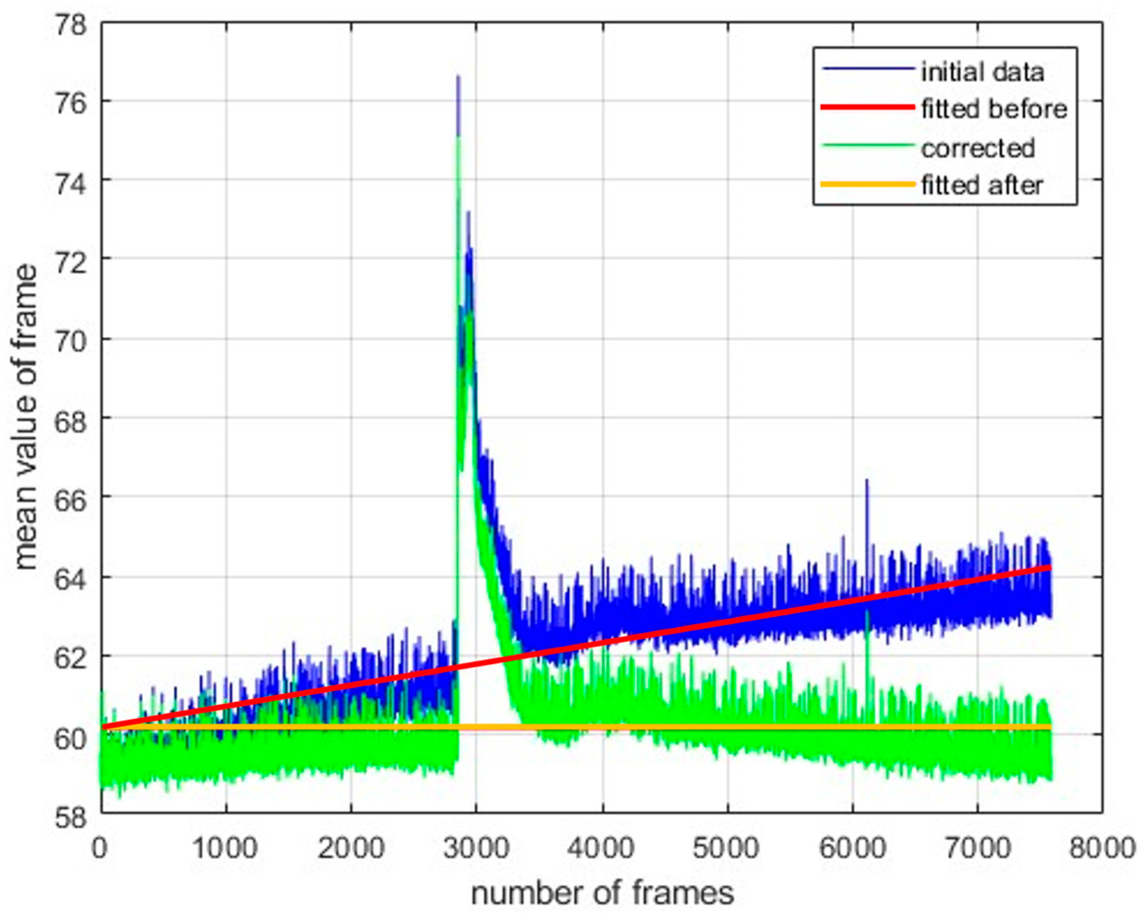
- Data preprocessing
- (4)
- Feature extraction:
- (5)
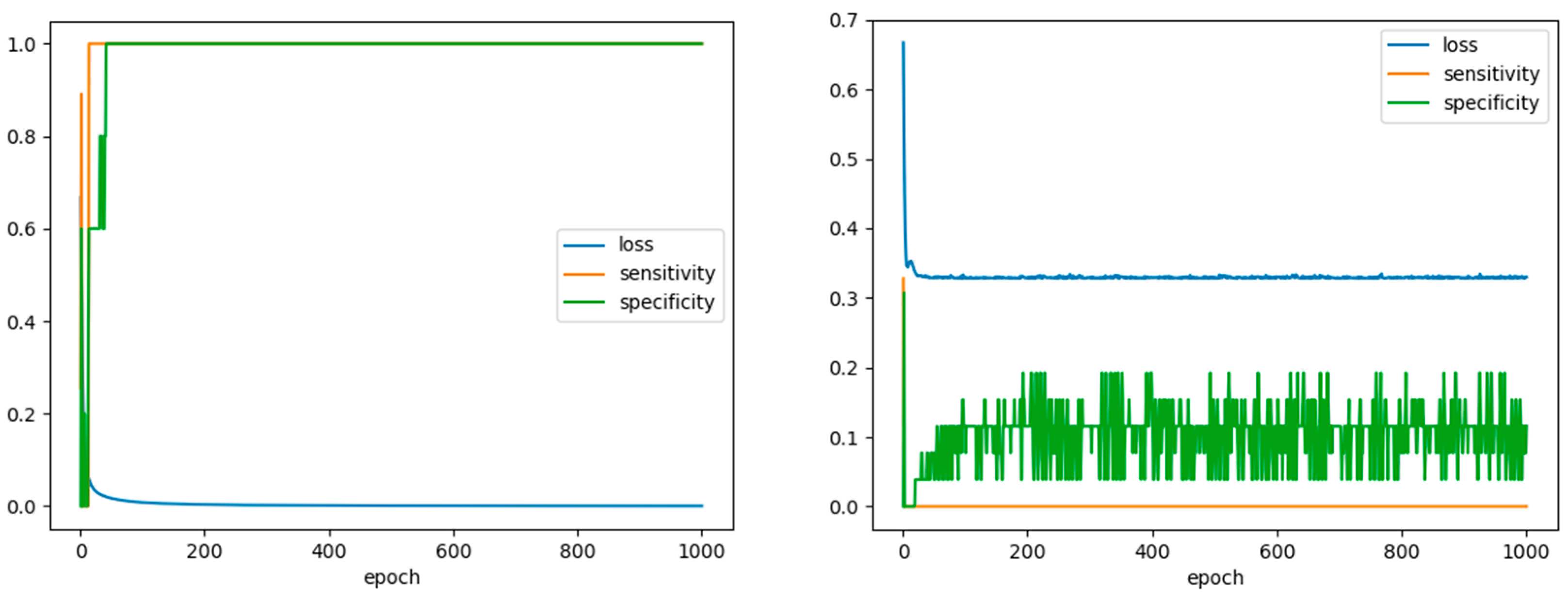
- Model training:
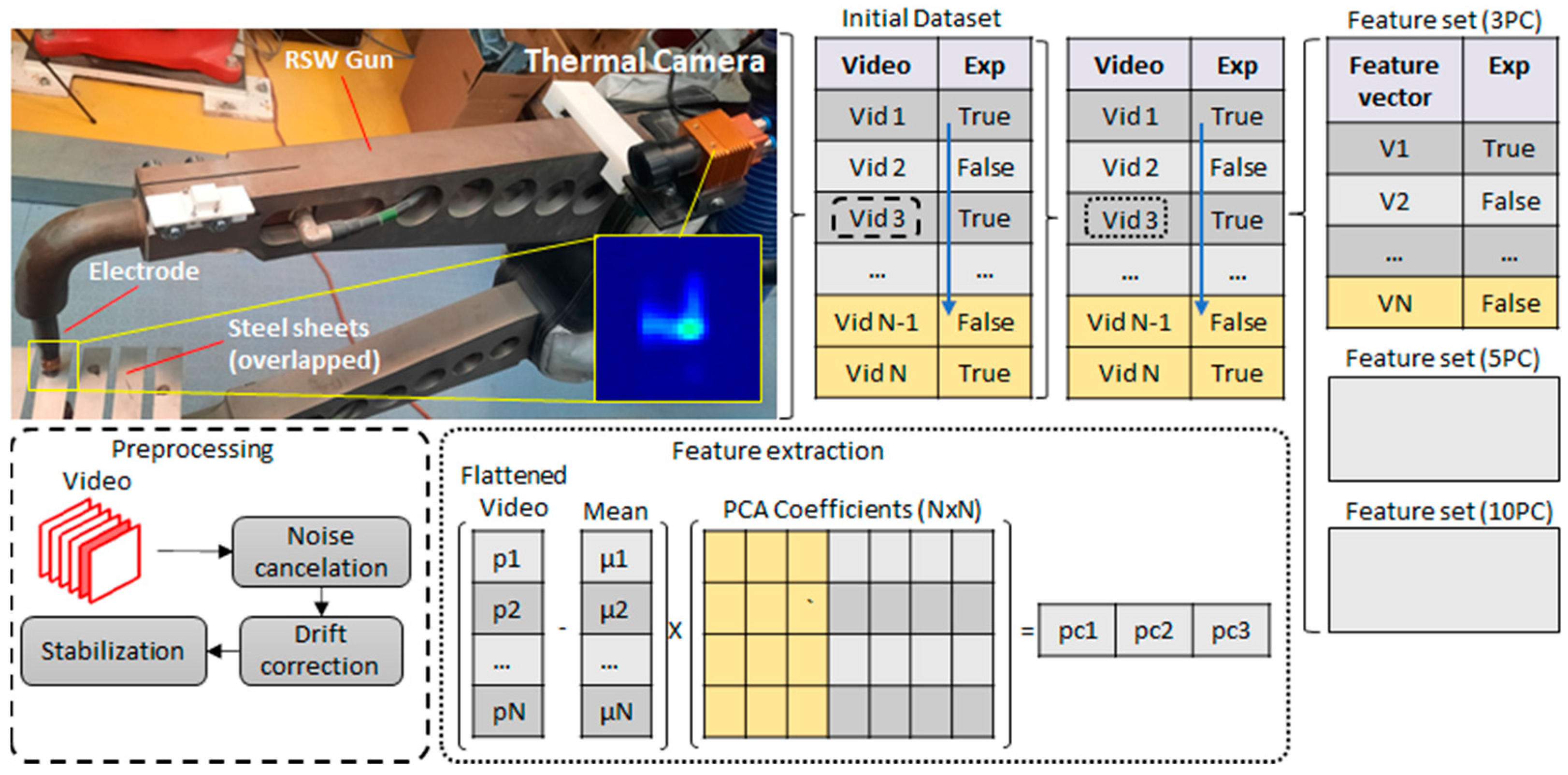
3.2. Case Study II
- Data pre-processing:
- 2.
- Feature extraction:
- 3.
- Model training:
4. Results
4.1. Laser Welding and Veracity
4.2. RSW Case: Veracity and Value
5. Discussion
6. Conclusions and Future Outlook
Author Contributions
Funding
Institutional Review Board Statement
Informed Consent Statement
Data Availability Statement
Conflicts of Interest
References
- Belhadi, A.; Zkik, K.; Cherrafi, A.; Sha’ri, M.Y. Understanding big data analytics for manufacturing processes: Insights from literature review and multiple case studies. Comput. Ind. Eng. 2019, 137, 106099. [Google Scholar] [CrossRef]
- Cui, Y.; Kara, S.; Chan, K.C. Manufacturing big data ecosystem: A systematic literature review. Robot. Comput.-Integr. Manuf. 2020, 62, 101861. [Google Scholar] [CrossRef]
- Helms, J. Big Data: It’s About Complexity, Not Size. IBM Center for The Business of Government. 2015. Available online: https://www.businessofgovernment.org/blog/big-data-it%E2%80%99s-about-complexity-not-size (accessed on 15 September 2023).
- Tunc-Abubakar, T.; Kalkan, A.; Abubakar, A.M. Impact of big data usage on product and process innovation: The role of data diagnosticity. Kybernetes 2022. [Google Scholar] [CrossRef]
- Papacharalampopoulos, A.; Michail, C.K.; Stavropoulos, P. Manufacturing resilience and agility through processes digital twin: Design and testing applied in the LPBF case. Procedia CIRP 2021, 103, 164–169. [Google Scholar] [CrossRef]
- Kortelainen, H.; Happonen, A.; Hanski, J. From asset provider to knowledge company—Transformation in the digital era. In Asset Intelligence through Integration and Interoperability and Contemporary Vibration Engineering Technologies; Springer: Cham, Switzerland, 2019; pp. 333–341. [Google Scholar]
- Alexopoulos, K.; Nikolakis, N.; Chryssolouris, G. Digital twin-driven supervised machine learning for the development of artificial intelligence applications in manufacturing. Int. J. Comput. Integr. Manuf. 2020, 33, 429–439. [Google Scholar] [CrossRef]
- Statista Research Department. Big Data—Statistics & Facts. Available online: https://www.statista.com/topics/1464/big-data/ (accessed on 7 April 2022).
- Statista Research Department. Advanced and Predictive Analytics Software Revenue Worldwide from 2013 to 2019. Available online: https://www.statista.com/statistics/1172729/advanced-and-predictive-analytics-software-revenue-worldwide/ (accessed on 7 April 2022).
- Statista Research Department. Analytics as a Service (AaaS) Market Size Forecast Worldwide in 2018 and 2026. Available online: https://www.statista.com/statistics/1234242/analytics-as-a-service-global-market-size/ (accessed on 7 April 2022).
- Stavropoulos, P.; Papacharalampopoulos, A.; Sabatakakis, K.; Mourtzis, D. Quality Monitoring of Manufacturing Processes based on Full Data Utilization. Procedia CIRP 2021, 104, 1656–1661. [Google Scholar] [CrossRef]
- Marx, V. The big challenges of big data. Nature 2013, 498, 255–260. [Google Scholar] [CrossRef]
- Muniswamaiah, M.; Agerwala, T.; Tappert, C. Big data in cloud computing review and opportunities. arXiv 2019, arXiv:1912.10821. [Google Scholar] [CrossRef]
- Tomaz, R.B. Big Data Analytics as a Service: How Can Services Influence Big Data Analytics Capabilities in Small and Mid-Sized Companies? Master’s Thesis, Federal University of Rio de Janeiro, Rio de Janeiro, Brazil, 2020. [Google Scholar]
- Gandomi, A.; Haider, M. Beyond the hype: Big data concepts, methods, and analytics. Int. J. Inf. Manag. 2015, 35, 137–144. [Google Scholar] [CrossRef]
- Rubin, V.; Lukoianova, T. Veracity roadmap: Is big data objective, truthful and credible? Adv. Classif. Res. Online 2013, 24, 4. [Google Scholar] [CrossRef]
- Reimer, A.P.; Madigan, E.A. Veracity in big data: How good is good enough. Health Inform. J. 2019, 25, 1290–1298. [Google Scholar] [CrossRef] [PubMed]
- Cappa, F.; Oriani, R.; Peruffo, E.; McCarthy, I. Big data for creating and capturing value in the digitalized environment: Unpacking the effects of volume, variety, and veracity on firm performance. J. Prod. Innov. Manag. 2021, 38, 49–67. [Google Scholar] [CrossRef]
- Stavropoulos, P.; Papacharalampopoulos, A.; Sabatakakis, K. Online Quality Inspection Approach for Submerged Arc Welding (SAW) by Utilizing IR-RGB Multimodal Monitoring and Deep Learning. In Proceedings of the International Conference on Flexible Automation and Intelligent Manufacturing, Detroit, MI, USA, 19–23 June 2022; pp. 160–169. [Google Scholar] [CrossRef]
- Segreto, T.; Teti, R. Data quality evaluation for smart multi-sensor process monitoring using data fusion and machine learning algorithms. Prod. Eng. 2023, 17, 197–210. [Google Scholar] [CrossRef]
- Stephens, Z.D.; Lee, S.Y.; Faghri, F.; Campbell, R.H.; Zhai, C.; Efron, M.J.; Iyer, R.; Schatz, M.C.; Sinha, S.; Robinson, G.E. Big data: Astronomical or genomical? PLoS Biol. 2015, 13, e1002195. [Google Scholar] [CrossRef]
- Rodríguez-Mazahua, L.; Rodríguez-Enríquez, C.A.; Sánchez-Cervantes, J.L.; Cervantes, J.; García-Alcaraz, J.L.; Alor-Hernández, G. A general perspective of Big Data: Applications, tools, challenges and trends. J. Supercomput. 2016, 72, 3073–3113. [Google Scholar] [CrossRef]
- IBM. How to Manage Complexity and Realize the Value of Big Data. Available online: https://www.ibm.com/blogs/services/2020/05/28/how-to-manage-complexity-and-realize-the-value-of-big-data/ (accessed on 28 May 2022).
- Agrawal, D.; Das, S.; El Abbadi, A. Big data and cloud computing: Current state and future opportunities. In Proceedings of the 14th International Conference on Extending Database Technology, New York, NY, USA, 21–24 March 2011; pp. 530–533. [Google Scholar] [CrossRef]
- Mourtzis, D.; Vlachou, E.; Milas, N. Industrial big data as a result of IoT adoption in manufacturing. Procedia CIRP 2016, 55, 290–295. [Google Scholar] [CrossRef]
- Rashid, Z.N.; Zebari, S.R.M.; Sharif, K.H.; Jacksi, K. Distributed cloud computing and distributed parallel computing: A review. In Proceedings of the International Conference on Advanced Science and Engineering, Duhok, Iraq, 9–11 October 2018. [Google Scholar]
- Vanani, I.R.; Majidian, S. Literature review on big data analytics methods. In Social Media and Machine Learning; IntechOpen: London, UK, 2019. [Google Scholar]
- UnnisaBegum, A.; Hussain, M.A.; Shaik, M. Data mining techniques for big data. Int. J. Adv. Res. Sci. Eng. Technol. 2019, 6, 396–399. [Google Scholar]
- Drineas, P.; Mahoney, M.W. RandNLA: Randomized numerical linear algebra. Commun. ACM 2016, 59, 80–90. [Google Scholar] [CrossRef]
- Wang, L.; Alexander, C.A. Additive manufacturing and big data. Int. J. Math. Eng. Manag. Sci. 2016, 1, 107. [Google Scholar] [CrossRef]
- Seyedan, M.; Mafakheri, F. Predictive big data analytics for supply chain demand forecasting: Methods, applications, and research opportunities. J. Big Data 2020, 7, 53. [Google Scholar] [CrossRef]
- Kamble, S.S.; Gunasekaran, A. Big data-driven supply chain performance measurement system: A review and framework for implementation. Int. J. Prod. Res. 2020, 58, 65–86. [Google Scholar] [CrossRef]
- Qiao, F.; Liu, J.; Ma, Y. Industrial big-data-driven and CPS-based adaptive production scheduling for smart manufacturing. Int. J. Prod. Res. 2021, 59, 7139–7159. [Google Scholar] [CrossRef]
- Jieyang, P.; Kimmig, A.; Dongkun, W.; Niu, Z.; Zhi, F.; Jiahai, W.; Liu, X.; Ovtcharova, J. A systematic review of data-driven approaches to fault diagnosis and early warning. J. Intell. Manuf. 2022, 34, 3277–3304. [Google Scholar] [CrossRef]
- Shang, C.; You, F. Data analytics and machine learning for smart process manufacturing: Recent advances and perspectives in the big data era. Engineering 2019, 5, 1010–1016. [Google Scholar] [CrossRef]
- Tsang, Y.P.; Wu, C.H.; Lin, K.Y.; Tse, Y.K.; Ho, G.T.S.; Lee, C.K.M. Unlocking the power of big data analytics in new product development: An intelligent product design framework in the furniture industry. J. Manuf. Syst. 2022, 62, 777–791. [Google Scholar] [CrossRef]
- Fronius International GmbH. Big Data in Welding Technology. Fronius International GmbH 2018. Available online: https://blog.perfectwelding.fronius.com/wp-content/uploads/2018/12/Fronius-PW_Whitepaper_Big-Data_EN-US.pdf (accessed on 14 April 2022).
- Ennsbrunner, H. Exploring the Role of Big Data in Welding Technology. Efficient Manufacturing 2019. Available online: https://www.industr.com/en/exploring-the-role-of-big-data-in-welding-technology-2360956 (accessed on 14 April 2022).
- Francis, J.; Bian, L. Deep learning for distortion prediction in laser-based additive manufacturing using big data. Manuf. Lett. 2019, 20, 10–14. [Google Scholar] [CrossRef]
- Jieyang, P.; Kimmig, A.; Wang, J.; Liu, X.; Niu, Z.; Ovtcharova, J. Dual-stage attention-based long-short-term memory neural networks for energy demand prediction. Energy Build. 2021, 249, 111211. [Google Scholar] [CrossRef]
- Zhou, L.; Wang, Ζ.; Luo, Υ.; Xiong, Z. Separability and compactness network for image recognition and superresolution. IEEE Trans. Neural Netw. Learn. Syst. 2019, 30, 3275–3286. [Google Scholar] [CrossRef]
- Song, W.; Shi, C.; Xiao, Z.; Duan, Z.; Xu, Y.; Zhang, M.; Tang, J. Autoint: Automatic feature interaction learning via self-attentive neural networks. In Proceedings of the 28th ACM International Conference on Information and Knowledge Management, Beijing, China, 3–7 November 2019; pp. 1161–1170. [Google Scholar] [CrossRef]
- Braun, M.; Kellner, L.; Schreiber, S.; Ehlers, S. Prediction of fatigue failure in small-scale butt-welded joints with explainable machine learning. Procedia Struct. Integr. 2022, 38, 182–191. [Google Scholar] [CrossRef]
- Beck, D.; Dechent, P.; Junker, M.; Sauer, D.U.; Dubarry, M. Inhomogeneities and Cell-to-Cell Variations in Lithium-Ion Batteries, a Review. Energies 2021, 14, 3276. [Google Scholar] [CrossRef]
- Yang, Y.; Pan, L.; Ma, J.; Yang, R.; Zhu, Y.; Yang, Y.; Zhang, L. A high-performance deep learning algorithm for the automated optical inspection of laser welding. Appl. Sci. 2020, 10, 933. [Google Scholar] [CrossRef]
- Ying, X. An overview of overfitting and its solutions. J. Phys. Conf. Ser. 2019, 1168, 022022. [Google Scholar] [CrossRef]
- Kingma, D.P.; Ba, J. Adam: A method for stochastic optimization. arXiv 2014, arXiv:1412.6980. [Google Scholar]
- Kumar, R.; Chohan, J.S.; Goyal, R.; Chauhan, P. Impact of process parameters of resistance spot welding on mechanical properties and micro hardness of stainless steel 304 weldments. Int. J. Struct. Integr. 2020, 12, 366–377. [Google Scholar] [CrossRef]
- Manladan, S.M.; Yusof, F.; Ramesh, S.; Fadzil, M.; Luo, Z.; Ao, S. A review on resistance spot welding of aluminum alloys. Int. J. Adv. Manuf. Technol. 2017, 90, 605–634. [Google Scholar] [CrossRef]
- Xia, Y.J.; Su, Z.W.; Li, Y.B.; Zhou, L.; Shen, Y. Online quantitative evaluation of expulsion in resistance spot welding. J. Manuf. Process. 2019, 46, 34–43. [Google Scholar] [CrossRef]
- Stavropoulos, P.; Sabatakakis, K.; Papacharalampopoulos, A.; Mourtzis, D. Infrared (IR) quality assessment of robotized resistance spot welding based on machine learning. Int. J. Adv. Manuf. Technol. 2022, 119, 1785–1806. [Google Scholar] [CrossRef]
- Møller, M.F. A scaled conjugate gradient algorithm for fast supervised learning. Neural Netw. 1993, 6, 525–533. [Google Scholar] [CrossRef]
- Stavropoulos, P.; Bikas, H.; Sabatakakis, K.; Theoharatos, C.; Grossi, S. Quality assurance of battery laser welding: A data-driven approach. Procedia CIRP 2022, 111, 784–789. [Google Scholar] [CrossRef]
- Stavropoulos, P.; Papacharalampopoulos, A.; Michail, C.K.; Chryssolouris, G. Robust additive manufacturing performance through a control oriented digital twin. Metals 2021, 11, 708. [Google Scholar] [CrossRef]
- Stavropoulos, P.; Papacharalampopoulos, A.; Sabatakakis, K. Robust and Secure Quality Monitoring for Welding through Platform-as-a-Service: A Resistance and Submerged Arc Welding Study. Machines 2023, 11, 298. [Google Scholar] [CrossRef]
- Luo, G.; Yuan, Q.; Li, J.; Wang, S.; Yang, F. Artificial Intelligence Powered Mobile Networks: From Cognition to Decision. arXiv 2021, arXiv:2112.04263. [Google Scholar] [CrossRef]


| # | Feature | Definition [14,15] |
|---|---|---|
| V1 | Volume | Represents the size of the dataset. |
| V2 | Velocity | Reflects the speed at which data are collected and analyzed. |
| V3 | Variety | Comes from the plurality of structured and unstructured data sources, such as text, videos, networks, and graphics, among others. |
| V4 | Variability | Constant change in data, i.e., in rate. |
| V5 | Veracity | Ensures that the data used are trusted, implying security among others. Herein, the concept of usability, as expressed through uncertainty [16], primarily, as well as completeness [17] will be addressed. |
| V6 | Visualization/Verification | Can be described as interpreting the patterns and trends present in the data. |
| V7 | Value | Represents the extent to which big data generates economically worthy insights and benefits through extraction and transformation. There are already clear statements that it is coupled with veracity, through the literature [18]. |
| Feature | Factors |
|---|---|
| Volume | 1. Process duration 2. Resolution of camera 3. Sampling rate of the camera |
| Velocity | Depending on the speed of the process monitoring; how many single frames per second (also on how many different files need handling)? |
| Variety | This has to do with the fact that the monitoring system may not rely only on one camera (single spectrum, or single angle) but on multispectral and stereo vision, possibly with different sampling rates. |
| Variability | This can be related to potential reuses of the system in different welding configurations or the use of the data in multiple control loops with different sampling rates. |
| Veracity | This depends on the combination of material and camera sensitivity, the thermal drift of the camera, and all the features that favor the introduction of noise, both from the camera itself (i.e., lambertian source) and the environment (background radiation). |
| Visualization/Verification | At a minimum, this is related to the ease of extracting features that can offer a good correlation with the ultimate goal of the application. |
| Value | Among technical factors, such as monitoring performance, business-wise, it could also be linked to explainable machine learning in the case of human-centric manufacturing [43]. |
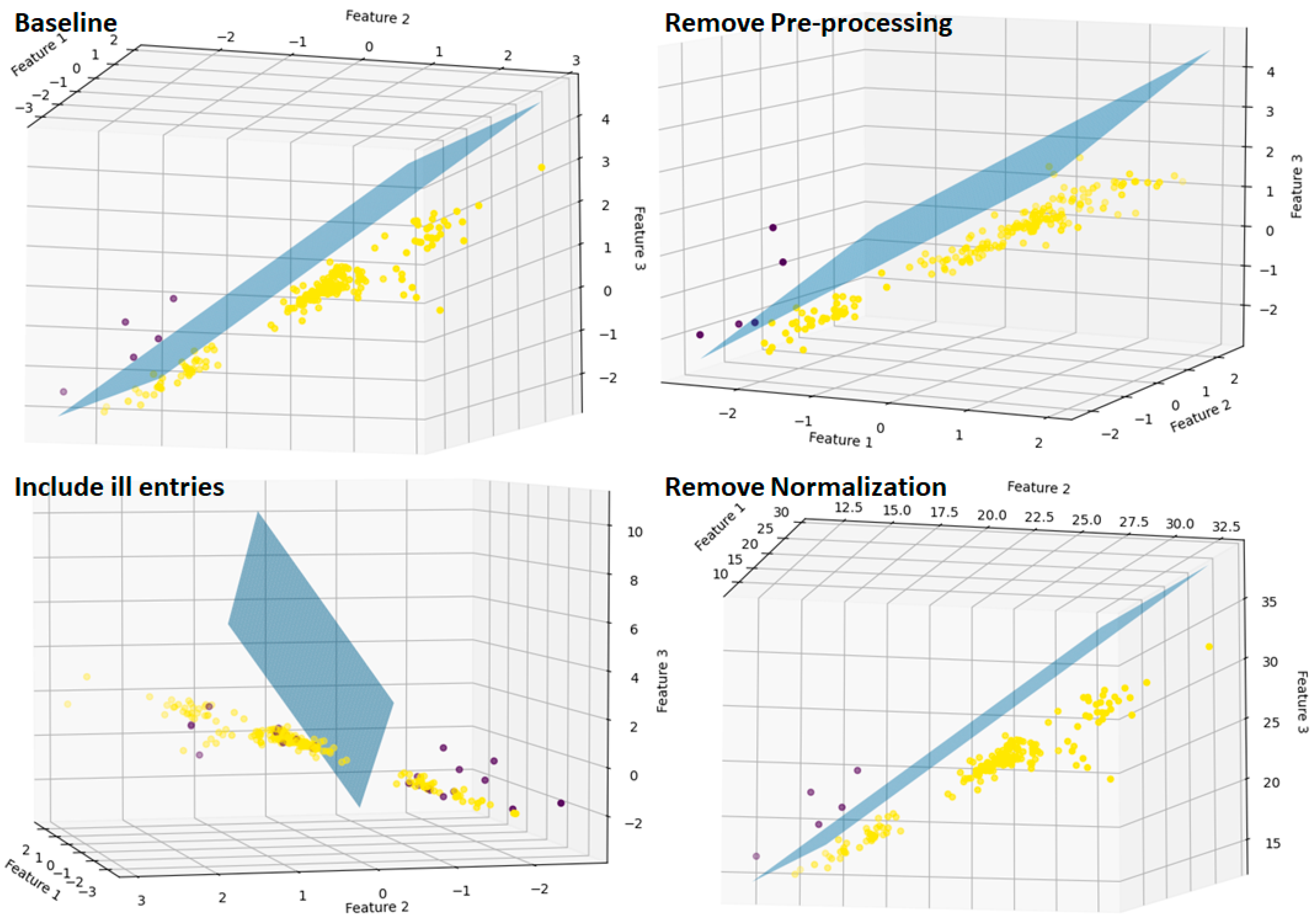
| Action | Description |
|---|---|
| (Removing) Data preprocessing steps | Remove noise-cancellation as already described in the previous step. |
| (Including) Ill entries | Leave entries that correspond to faulty ECR measurements. |
| (Removing) Normalization | Do not scale the features. |
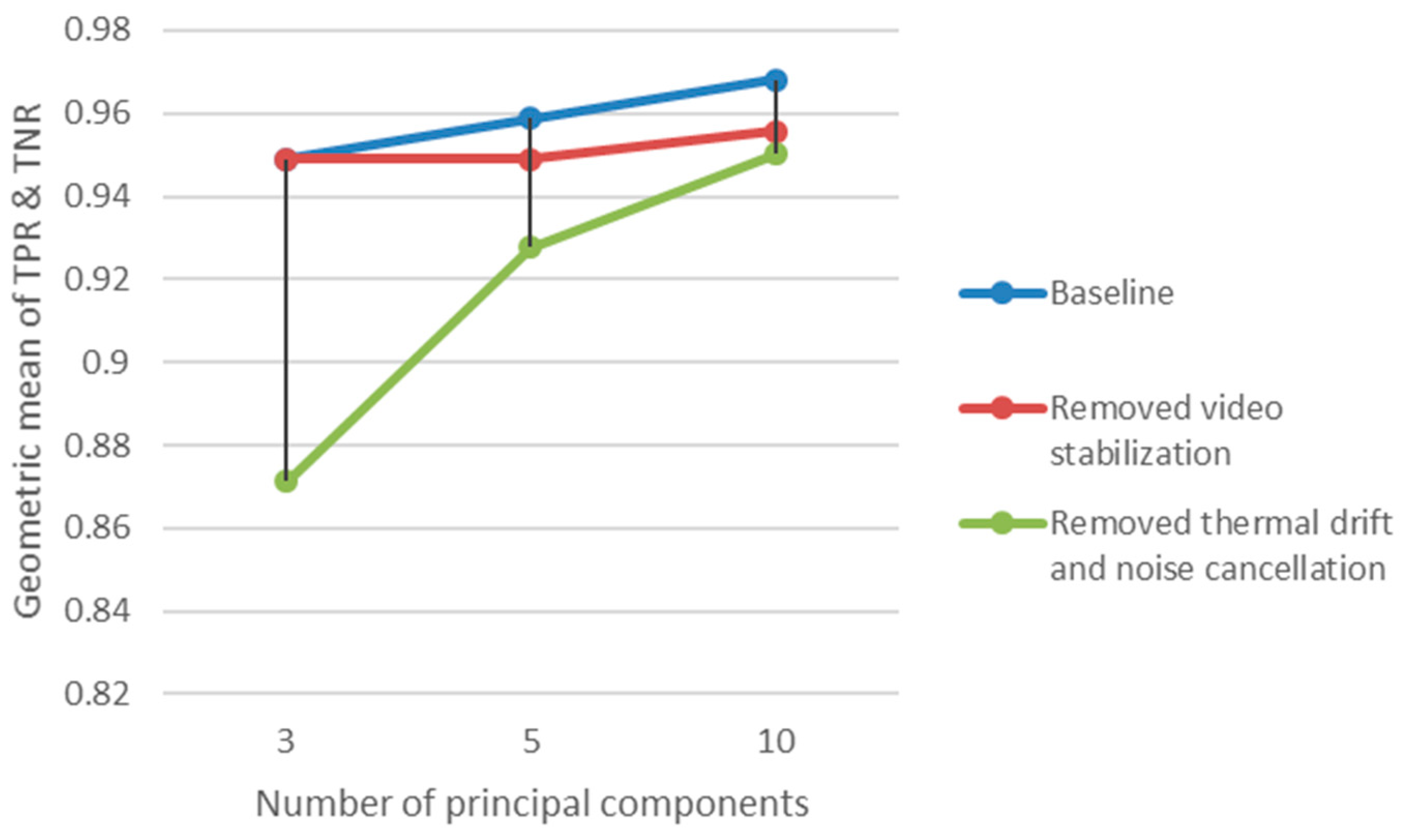
| Veracity Code | Veracity Factor | Value Code | Value Factor |
|---|---|---|---|
| P1 | All steps included | F1 | PCA: 3PC |
| P2 | Remove video stabilization | F2 | PCA: 5PC |
| P3 | Remove thermal-drift correction and noise cancelation | F3 | PCA: 10PC |
| F1 | F2 | F3 | |||||||
|---|---|---|---|---|---|---|---|---|---|
| TPR | TNR | Epochs | TPR | TNR | Epochs | TPR | TNR | Epochs | |
| P1 | 0.907 | 0.993 | 35 | 0.926 | 0.993 | 230 | 0.944 | 0.993 | 375 |
| P2 | 0.907 | 0.993 | 200 | 0.907 | 0.993 | 200 | 0.92 | 0.993 | 200 |
| P3 | 0.782 | 0.971 | 75 | 0.873 | 0.986 | 274 | 0.909 | 0.993 | 689 |
Disclaimer/Publisher’s Note: The statements, opinions and data contained in all publications are solely those of the individual author(s) and contributor(s) and not of MDPI and/or the editor(s). MDPI and/or the editor(s) disclaim responsibility for any injury to people or property resulting from any ideas, methods, instructions or products referred to in the content. |
© 2023 by the authors. Licensee MDPI, Basel, Switzerland. This article is an open access article distributed under the terms and conditions of the Creative Commons Attribution (CC BY) license (https://creativecommons.org/licenses/by/4.0/).
Share and Cite
Stavropoulos, P.; Papacharalampopoulos, A.; Sabatakakis, K. Data Attributes in Quality Monitoring of Manufacturing Processes: The Welding Case. Appl. Sci. 2023, 13, 10580. https://doi.org/10.3390/app131910580
Stavropoulos P, Papacharalampopoulos A, Sabatakakis K. Data Attributes in Quality Monitoring of Manufacturing Processes: The Welding Case. Applied Sciences. 2023; 13(19):10580. https://doi.org/10.3390/app131910580
Chicago/Turabian StyleStavropoulos, Panagiotis, Alexios Papacharalampopoulos, and Kyriakos Sabatakakis. 2023. "Data Attributes in Quality Monitoring of Manufacturing Processes: The Welding Case" Applied Sciences 13, no. 19: 10580. https://doi.org/10.3390/app131910580
APA StyleStavropoulos, P., Papacharalampopoulos, A., & Sabatakakis, K. (2023). Data Attributes in Quality Monitoring of Manufacturing Processes: The Welding Case. Applied Sciences, 13(19), 10580. https://doi.org/10.3390/app131910580