Time-Sensitive and Resource-Aware Concurrent Workflow Scheduling for Edge Computing Platforms Based on Deep Reinforcement Learning

Abstract

The workflow scheduling on edge computing platforms in industrial scenarios aims to efficiently utilize the computing resources of edge platforms to meet user service requirements. Compared to ordinary task scheduling, tasks in workflow scheduling come with predecessor and successor constraints. The solutions to scheduling problems typically include traditional heuristic methods and modern deep reinforcement learning approaches. For heuristic methods, an increase in constraints complicates the design of scheduling rules, making it challenging to devise suitable algorithms. Additionally, whenever the environment undergoes updates, it necessitates the redesign of the scheduling algorithms. For existing deep reinforcement learning-based scheduling methods, there are often challenges related to training difficulty and computation time. The addition of constraints makes it challenging for neural networks to make decisions while satisfying those constraints. Furthermore, previous methods mainly relied on RNN and its variants to construct neural network models, lacking a computation time advantage. In response to these issues, this paper introduces a novel workflow scheduling method based on reinforcement learning, which utilizes neural networks for direct decision-making. On the one hand, this approach leverages deep reinforcement learning, eliminating the need for researchers to define complex scheduling rules. On the other hand, it separates the parsing of the workflow and constraint handling from the scheduling decisions, allowing the neural network model to focus on learning how to schedule without the necessity of learning how to handle workflow definitions and constraints among sub-tasks. The method optimizes resource utilization and response time, as its objectives and the network are trained using the PPO algorithm combined with Self-Critic, and the parameter transfer strategy is utilized to find the balance point for multi-objective optimization. Leveraging the advantages of reinforcement learning, the network can be trained and tested using randomly generated datasets. The experimental results indicate that the proposed method can generate different scheduling outcomes to meet various scenario requirements without modifying the neural network. Furthermore, when compared to other deep reinforcement learning methods, the proposed approach demonstrates certain advantages in scheduling performance and computation time.

1. Introduction

Currently, industrial Internet of Things (IoT) applications are continuously evolving towards deeper integration, where all elements of industrial processes are interconnected. Data from various sources, such as physical sensors, images, audio, and video, are constantly collected and accumulated [1]. Real-time intelligent analysis and processing of process monitoring data are often required to achieve timely feedback and optimization control of production processes. The demand for real-time data collection and processing in industrial scenarios based on edge computing is rapidly growing [2]. These data-intensive storage and computing tasks, carried out at the edge, heavily rely on computational and storage resources, and have stricter requirements for real-time execution of workflows [3].

Typically, the analysis and processing of heterogeneous data from multiple sources in industrial processes involves various steps, including data acquisition, data correlation analysis, AI inference, and industrial equipment feedback control. These steps form a workflow with multiple sub-tasks that need to be executed collaboratively and in real-time [4]. Moreover, due to the concurrent nature of real-time data processing tasks in industrial processes (e.g., device operation condition monitoring and fault diagnosis, product quality inspection, and optimization during production), edge computing platform are required to run multiple sub-tasks concurrently as part of the workflow. The real-time scheduling of these concurrent workflows on resource-constrained edge computing platforms, including computation and storage, poses a critical challenge for current industrial IoT edge computing [3,5].

The issue of concurrency in cloud computing or edge computing can be considered the same type of problem. In recent years, real-time scheduling of concurrent tasks and workflow scheduling on cloud computing or edge computing have received special attention from researchers [3,6,7]. The optimization objectives in such studies mostly focus on resources, QoS, and time. The methods employed for scheduling are predominantly heuristic, including rule-based and search-based methods. A small portion of the research has utilized deep learning methods, primarily for assessing the effectiveness of solutions using neural networks, rather than having the neural networks make decisions. These heuristic methods often lack analysis of computation time in experiments. However, it can also be observed that researchers are gradually integrating the latest deep learning research into traditional methods for such problems.

The traditional methods for solving scheduling problems are primarily heuristic methods, which can be further classified into two categories. The first class are rule-based heuristic scheduling methods, which typically rely on predefined rules for scheduling without optimizing the scheduling results. The second class belongs to search-based heuristic algorithms. This method often utilizes various rules to search the solution space and find a feasible solution to the optimization problem within acceptable costs (time or space), which is close to the optimal solution. Up to now, there have been numerous metaheuristic works on cloud/edge computing scheduling [8]. Examples of such methods include Particle Swarm Optimization (PSO) [9,10], Ant Colony Optimization (ACO) [11], and Differential Evolution (DE) [12], which have been adopted to optimize the makespan or cost (e.g., resource cost) while satisfying other QoS constraints. It is worth noting that the makespan and cost of executing a workflow on the cloud are two conflicting optimization objectives. For instance, reducing the makespan of the workflow requires more resources, which often leads to higher execution costs. As a result, many algorithms struggle to strike a balance between these two objectives. Furthermore, such methods often face challenges in meeting the real-time requirements of certain scenarios.

In recent years, with the development of artificial intelligence, Reinforcement Learning (RL) has become an active area of research in machine learning [13,14]. Its ability to address decision-making problems has inspired researchers to use RL to tackle optimization problems. Most research leverages Deep Reinforcement Learning (DRL) to learn solutions for problem-solving by designing evaluation metrics for the problem and enabling neural networks to continuously attempt and learn through trial. With the trained network, excellent solutions can be obtained in a short amount of time. Many studies have utilized Deep Reinforcement Learning to solve resource management problems [15], workshop job scheduling problems [16], and cloud-edge task allocation problems [17]. While using Deep Reinforcement Learning methods can avoid designing highly complex heuristic rules and offer faster computation times, there are still challenges in designing the environment states and network models, as well as the need to balance different optimization objectives.

Many heuristic methods utilize search and neural 94 network techniques, but their computational efficiency falls short in real-time scheduling 95 environments.

Previous research has encountered several challenges: (1) Heuristic methods often require the design of overly complex rules, and scheduling rules need to be designed while satisfying problem constraints. When the constraints change, the scheduling rules may need to be modified accordingly. The methods of deep reinforcement learning become increasingly challenging to train as the problem constraints increase, leading to an increase in the required input features. (2) Many scheduling methods, while capable of producing excellent results, have computation times that are unacceptable for real-time environments. (3) Dealing with multi-objective optimization requires frequent adjustments to algorithm rules or neural networks to find a balanced point among multiple objectives. To address these issues, this paper adopts the Deep Reinforcement Learning (DRL) method and designs an intelligent scheduler to solve the sub-task scheduling problem on edge servers in industrial scenarios. The scheduler separates problem constraints from the problem-solving process, with the neural network solely responsible for solving the input problem without considering the constraints, which are controlled by the non-neural-network part. The scheduler optimizes two metrics: resource utilization and response time, with low computation time. The contributions of this paper are as follows:

• An intelligent scheduler was designed to separate the parsing of the environment from the scheduling decisions. The workflow meta-data and current environment are used to generate masks and environment encoding, which are then fed back to the neural network. The neural network is trained using the PPO algorithm combined with the Self-Critic mechanism to learn how to schedule;
• Based on the pointer network architecture, the neural network was designed using Transformer as the foundation. This neural network can efficiently process the features of sub-tasks, significantly improving the computation speed of the scheduler in real-time environments;
• For multi-objective optimization problems, a parameter transfer strategy is applied to transfer parameters rapidly and efficiently across multiple sets of reward functions. This allows for the verification of how reward functions affect scheduling performance, leading to the selection of the optimal reward function.

The remaining sections of the article are as follows: Section 2 will provide a detailed overview of solutions to similar problems and explore how previous research has applied deep reinforcement learning methods to address other challenges. Section 3 will present a comprehensive description of the specific problems addressed in this study. In Section 4, the proposed model, along with some state parameters and scheduling strategies, will be introduced. The training methodology for the model will be discussed in Section 5. Section 6 will provide some experimental details and present the experimental results. Finally, Section 7 concludes.

2. Related Works

This section briefly describes methods for solving the scheduling problem and resource management problem, and work on deep reinforcement learning to solve problems in other domains.

2.1. Task Scheduling and Resource Management

Scheduling problems are crucial in various domains, with each scenario having unique details and distinct optimization objectives. Properly scheduling tasks (requests, jobs, etc.) not only enhances response speed, but also controls resource utilization and optimizes other performance metrics and costs as per the scenario requirements.

Table 1. Related work on solving scheduling problems.

Work	Problem	Method	Objective
Wang et al. [18]	Task scheduling and resource allocation	Search-based heuristic method; Annealing fusion algorithm	Minimize time delay and energy consumption
Liao et al. [19]	Task scheduling	Rule-based heuristic method; Set scheduling rules	Maximize average completion ratio
Sun et al. [20]	Workflow scheduling	Search-based heuristic method; Greedy search algorithm	Minimize makespan
Zhao et al. [21]	Job scheduling	Search-based heuristic method; Ant colony algorithm	Minimize execution overhead and timeliness
Mao et al. [15]	Resource management	Neural networks generate result; Policy gradient	Minimize average job slowdown
Mondal et al. [22]	Resource management	Neural networks generate result; Policy gradient	Maximize average resource utilization
Dong et al. [23]	Workflow scheduling	Neural networks generate result; Actor-Critic; Pointer network (RNN-based)	Minimize makespan
Chen et al. [24]	Job scheduling	Neural networks search result; DRL method; Actor-Critic; LSTM	Minimize average job slowdown
Ju et al. [25]	Computation offloading and tasks scheduling	Neural networks search; Actor-Critic; Pointer network (CNN-based)	Minimize timeout ratio and energy consumption
Ou et al. [26]	Satellite range scheduling problem	Neural networks generate result and rule-based heuristic method; Actor-Critic; Pointer network (Transformer-based)	Maximize number of scheduled tasks and profit

summarizes the problems addressed by these works and their respective methods.

Most of the mainstream methods for scheduling problems are based on heuristic algorithms. Wang et al. [18] proposed a genetic simulated annealing fusion algorithm to achieve task scheduling and resource allocation for cloud-edge collaborative architecture. Liao et al. proposed a two-stage scheduling method based on priority rules in their study [19]. This method involves scheduling among servers and within servers separately, based on the estimated task priorities. Additionally, it adjusts the priorities of subsequent tasks based on the actual start times of previous tasks. Sun et al. [20] presented a series of task allocation strategies for workflow scheduling in edge environments to accommodate different types of tasks. These strategies were combined with a greedy method to construct an improved greedy search algorithm. Zhao et al. [21] designed a parallel job scheduling algorithm that combines ant colony algorithm to address edge cloud-based scheduling problems.

In recent years, some researchers have applied deep reinforcement learning methods to various scheduling problems. Mao et al. [15] proposed a Policy Gradient-based method that considers both CPU and memory utilization. Task allocation is represented as a two-dimensional tabular image, with resource consumption on the horizontal axis and timestamps on the vertical axis, and task assignment is directly performed based on this table. Mondal et al. [22] developed a similar model to Mao et al. [15] for scheduling time-varying workloads in a shared cluster. They added multiple penalty terms to the reward function to avoid unreasonable decisions. Dong et al. [23] designed an RL agent based on the Pointer Network [27] to determine the execution sequence of workflows on heterogeneous cloud servers. They take the task sequence to be scheduled as input and obtain a sequence of machine-task assignments. Chen et al. [24] introduced a rewriter to solve job scheduling. They use a directed acyclic graph to represent the execution order of jobs. They construct an initial feasible solution randomly and then apply the rewriter on the graph to perform a local search, aiming to minimize the makespan as much as possible. Ju et al. [25] utilized the Pointer Network to address the problem of the edge platform being unable to simultaneously meet the real-time requirements of different tasks in the vehicular edge-collaborative environment. They proposed a multi-stage scheduling strategy to determine whether a task should be executed locally and also decide the task scheduling order within the edge server to meet the real-time requirements as much as possible. Ou et al. [26] combined DRL with heuristic methods to solve the satellite range scheduling problem (SRSP). They used neural network to learn the characteristics of satellite missions for task allocation to suitable antennas and used a heuristic method inside the antennas to select appropriate time windows for satellite communication. It can be observed that deep reinforcement learning methods have been applied in various scheduling domains with different scenarios, which also provides a practical foundation for this work.

2.2. Deep Reinforcement Learning for Solving Optimization Problems

Deep reinforcement learning is used to address optimization problems, and researchers’ main focus can be divided into two aspects. First is how to design the neural network. Second is the choice of training algorithms, which has a greater impact on the effectiveness of the neural network. Table 2 summarizes the problems addressed by these works and the methods employed.

Vinyals et al. [27] proposed the Pointer Network to solve the Traveling Salesman Problem (TSP). The authors analogized the combinatorial optimization problem to a machine translation problem (i.e., sequence-to-sequence mapping). The neural network’s input is a sequence of problem features (e.g., city coordinates), and the output is the solution sequence (e.g., the visiting order of cities). This research provided a strong model foundation for subsequent studies and serves as the model architecture adopted in this paper. However, this work still does not fall within the scope of reinforcement learning.

Bello et al. [28] were the first to propose using deep reinforcement learning to train the Pointer Network. They employed the Asynchronous Advantage Actor-Critic (A3C) [29] method to train the Pointer Network introduced by Vinyals. For the TSP, the authors considered selecting a city as an action, the current position as the state, and the total tour length as the reward, where lower length signifies a better result. Nazari et al. [30] addressed the Vehicle Routing Problem (VRP) and made partial modifications to the Pointer Network structure to reduce encoding time for user demands. They used the Actor-Critic method to solve the regular VRP and employed the A3C method to handle the stochastic VRP with random customer insertions. Ma et al. [31] combined the Pointer Network with Graph Neural Networks (GNN) to create a Graph Pointer Network for solving large-scale TSP and TSP problems with time window constraints. In addition to the original RNN Encoder, they used GNN to encode all cities and obtain graph embeddings. Kool et al. [32] replaced the RNN with the Transformer structure to design the Pointer Network and solved TSP, VRP, and other problems. The performance of their model surpassed that of the original Pointer Network. Lu et al. [33] designed operators to support transitions from one solution to another and trained a neural network through Policy Gradient to select operators, guiding the process of searching for solutions. Wu et al. [34] also used neural network to guide the process of searching for solutions, but they did not design operators. Instead, they let the network learn how to search for solutions.

It can be observed that in the field of deep reinforcement learning, there are two mainstream methods for solving optimization problems: one is to directly output optimization results through neural networks, and the other is to use neural networks to guide the direction of a heuristic search or directly perform the search, combining neural networks with heuristic methods. Although most of these studies focus on theoretical problems and have not addressed practical issues, the methods they propose provide a theoretical foundation for solving real-world scenarios.

Table 2. Related work on using deep reinforcement learning to address other problems.

Work	Problem	Method	Objective
Vinyals et al. [27]	TSP	Neural networks generate result (not DRL); Pointer network (RNN-based);	Minimize total tour length
Bello et al. [28]	TSP	Neural networks generate result; Pointer network (RNN-based); Actor-Critic;	Minimize total tour length
Nazari et al. [30]	VRP	Neural networks generate result; Pointer network (CNN and RNN); Actor-Critic	Minimize total tour length
Ma et al. [31]	TSP with variations	Neural networks generate result; Pointer network (GNN and LSTM); Policy gradient	Minimize total tour length
Kool et al. [32]	TSP, VRP and routing problem	Neural networks generate result; Transformer; Policy gradient	Minimize total tour length
Lu et al. [33]	VRP	Neural networks search result; Policy gradient	Minimize total tour length
Wu et al. [34]	TSP and CVRP	Neural networks search result; Policy gradient	Minimize total tour length

Table 2. Related work on using deep reinforcement learning to address other problems.

Work	Problem	Method	Objective
Vinyals et al. [27]	TSP	Neural networks generate result (not DRL); Pointer network (RNN-based);	Minimize total tour length
Bello et al. [28]	TSP	Neural networks generate result; Pointer network (RNN-based); Actor-Critic;	Minimize total tour length
Nazari et al. [30]	VRP	Neural networks generate result; Pointer network (CNN and RNN); Actor-Critic	Minimize total tour length
Ma et al. [31]	TSP with variations	Neural networks generate result; Pointer network (GNN and LSTM); Policy gradient	Minimize total tour length
Kool et al. [32]	TSP, VRP and routing problem	Neural networks generate result; Transformer; Policy gradient	Minimize total tour length
Lu et al. [33]	VRP	Neural networks search result; Policy gradient	Minimize total tour length
Wu et al. [34]	TSP and CVRP	Neural networks search result; Policy gradient	Minimize total tour length

3. Problem Description

This section will provide a detailed introduction to the proposed problem, including the structure of the scheduling scenario and the mathematical definition of the problem.

3.1. Edge Workflow Computing Platform Architecture

The edge workflow computing platform is primarily used to address collaborative work scenarios involving multiple services in edge environments. In an industrial environment, it is common practice to “embed” the execution flow of hardware or software into their respective code. This approach, on the one hand, leads to high coupling between individual hardware or software, and on the other hand, results in significant idle time for hardware or software. On the Edge Workflow Computing Platform, a variety of services are running, such as hardware control services, data storage services, and AI services. Compared to “embedding” process flows into these services, the interaction between these services is defined through workflows. In this scenario, the same service can simultaneously serve different workflows, significantly increasing service utilization. However, at the same time, the system’s complexity also increases, requiring the design of additional modules to control the execution of different workflows to ensure that tasks within the workflows are correctly processed by the corresponding service. For this purpose, a workflow design and execution platform has been developed to address this issue.

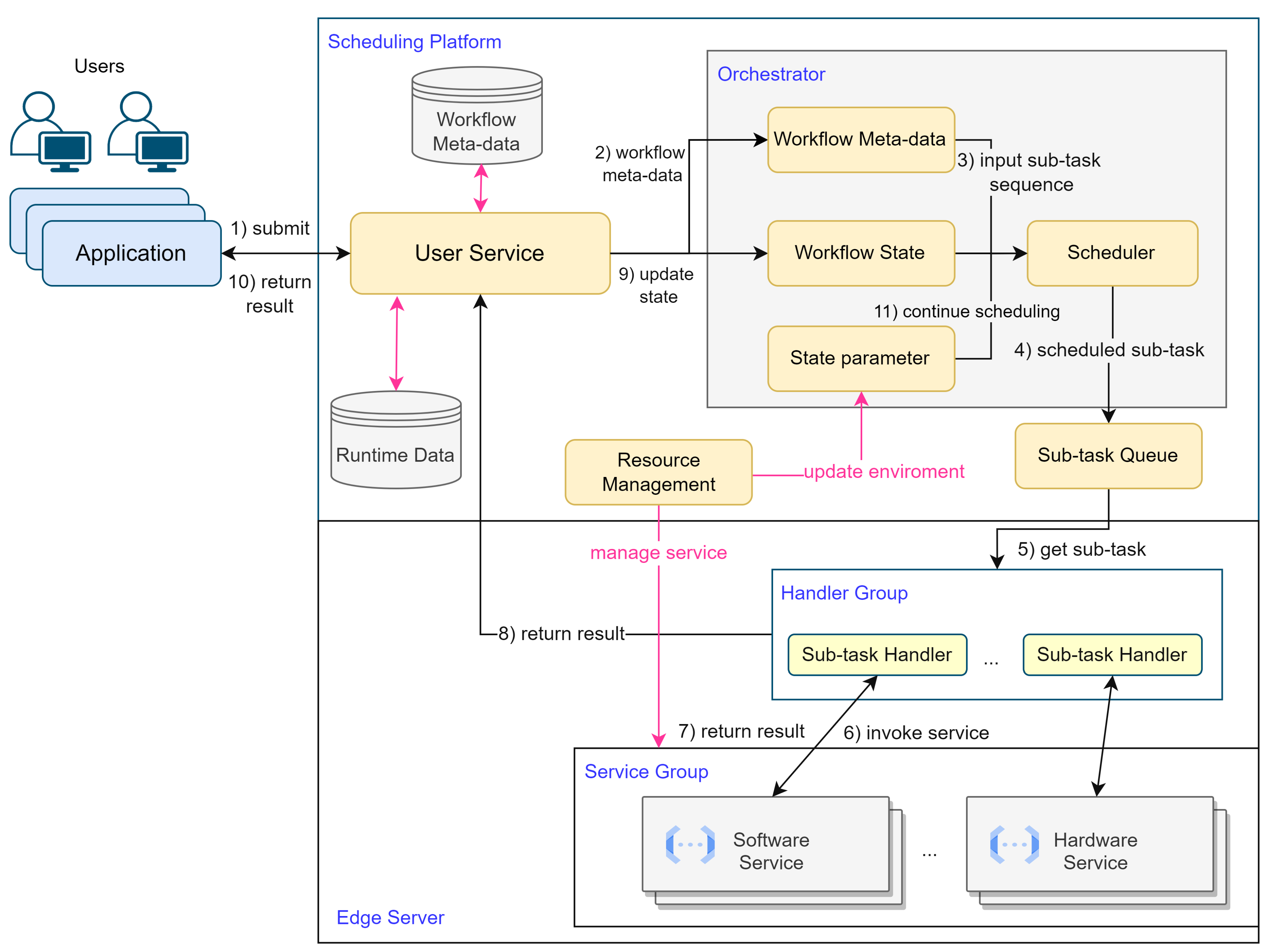
The structure of the entire system is illustrated in Figure 1. Users design and submit workflows through the user service. The Management Service is responsible for providing real-time feedback on execution information to users and receiving workflows from users to be handed over to the Orchestrator. The Orchestrator is the designated location for running the proposed method and is responsible for deciding which tasks should be added to the task queue. The task queue holds all scheduled and pending tasks for execution. The Edge Server runs the corresponding services that handle sub-tasks. The Resource Manager is responsible for monitoring the resource usage in edge servers and providing feedback to the Orchestrator.

Services can concurrently process sub-tasks when there are sufficient computational resources available. However, adding too many sub-tasks to the task queue results in a large number of tasks that services have to handle simultaneously. This can lead to resource competition among services, causing delayed completion times for multiple sub-tasks. Therefore, the scheduling objective is to balance the execution of sub-tasks across different workflows, minimizing overall response time while avoiding resource competition, and optimizing resource utilization. The Orchestrator parses all the workflows and extracts sub-tasks as an input sequence, denoted as $V=\{v_1,v_2,\dots ,v_{\left|V\right|}\}$, which is fed into the neural network. Based on the output results $O=\{o_1,o_2,\dots ,o_{\left|V\right|}\}$, the sub-tasks are scheduled. Figure 2 illustrates a case of workflow scheduling.

3.2. Entity Definitions and Constraints

In the edge workflow computing platform, there are three key entities: workflow, sub-task, and edge server. This subsection provides detailed definitions for these three entities and specifies the constraints during the scheduling process.

A workflow consists of multiple sub-tasks, where each sub-task has its predecessors and successors. The following symbols are used to describe the workflow model:

• $Workflows$: a collection of workflows submitted by users, containing a total of N workflows. $Workflow=\{w^1,w^2,\dots ,w^N\}$;
• $w^i$: a workflow is represented as a DAG and using adjacency matrix to represent DAG;
• $s{t}_j^i$: a sub-task in $w^i$;
• $x_{j,k}^i$: The elements in the matrix corresponding to $w^i$. Specifically, $x_{j,k}^i=1$ if $s{t}_j^i$ is the predecessor of $s{t}_k^i$, and $x_{j,k}^i=0$ for all other cases;
• i: the index of workflow.

The workflow model is responsible for maintaining the constraints between sub-tasks, while each sub-task has its own attributes. Each sub-task can be represented as a tuple of ($C_j^i$, $E_j^i$, $A{T}_j^i$, $D_j^i$, $P_j^i$).

• $C_j^i$: the Service corresponding to $s{t}_j^i$;
• $E_j^i$: the execution time of $s{t}_j^i$;
• $A{T}_j^i$: the arrival time of the sub-task;
• $D_j^i$: The resource requirements of $s{t}_j^i$. $D_j^i=\{r_1,r_2,\dots ,r_d\}$, where d represents the number of resources. Each resource requirement lies in the range $[0,1]$;
• $P_j^i$: the execution priority of $s{t}_j^i$;
• j: the index of sub-task;
• $SA{T}_j^i$: The start time of $s{t}_j^i$. This parameter is obtained by scheduling result.

The parameters of the edge server constrain the scheduling of sub-tasks. The definitions of the parameters relevant to the problem are as follows:

• $R_{edge}$: the resource for edge server. $R_{edge}=\{R_1,R_2,\dots ,R_d\}$;
• d: the index of Resource;
• t: the timestamp for edge server.

During scheduling, the parameters are subject to the following constraints:

• Time constraint: $SA{T}_j^i\ge Max\{SA{T}_k^i+E_k^i\}$, $\forall x_{k,j}^i=1$;
• Resource constraint: $R_{edge}\ge D_j^i$, when $s{t}_j^i$ can be scheduled.

For constraint (1), the actual start time of a sub-task, denoted as $SA{T}_j^i$, must satisfy the condition $SA{T}_j^i\ge Max\{SA{T}_k^i+E_k^i\}$. Here, $\{SA{T}_k^i+E_k^i\}$ represents the set of completion times of all predecessor sub-tasks. This constraint ensures that $s{t}_j^i$ cannot be executed before its predecessor sub-tasks have been completed.

For constraint (2), before adding a sub-task to the Sub-Task queue, it is crucial to verify that the computational resources available in the edge server can adequately meet the computational resource requirements for processing that Sub-Task.

In addition, the following constraints exist during scheduling:

• There will be no relationship between sub-tasks in different workflows;
• The time taken to transmit sub-tasks to the Sub-Task Queue and assemble the returned results is disregarded. The actual transmission time from the scheduling center to the edge servers can be determined through testing;
• Once a Service is processing a sub-task during runtime, it cannot be preempted or suspended;
• Upon completing a task, the Service can promptly release the allocated resources. Only the resources necessary for the Service to run are reserved.

3.3. Optimization Objective

In the proposed edge workflow computing platform, response time and resource consumption are the two key objectives (additional metrics can also be included), but these two objectives conflict with each other. On the one hand, the computing platform should to minimize the response time for each sub-task as much as possible. On the other hand, it should not excessively burden the system, as high loads can lead to longer execution times for all sub-tasks, rendering quick responses meaningless. Since both objectives need to be minimized, the overall scheduling objective is to find a balance point between these two objectives. As this paper employs a reinforcement learning method, the terms “reward” and “objective” are used interchangeably in the following text.

3.3.1. Average Resource Utilization

The ability of a Service to process a task is determined by its multiple resources together. Multiple resources are defined as parameters of the same type, all with values in the range [0, 1]. The total reward of the defined resources in this problem is as follows:

$$rewar{d}_1=\frac{{\sum }_{a=1}^d{\sum }_{i=0}^{t-1}R(T_i,r_a)(T_{i+1}-T_i)}{(T_t-T_0)\times d}$$

(1)

where $R(T_i,r_a)$ represents the usage of resource $r_a$ from $T_i$ to $T_{i+1}$. $T_i$ represents a timestamp. d represents the total number of resource types. The proposed platform defines four resources: CPU, GPU, memory, and I/O utilization.

3.3.2. Weighted Average Response Time and Penalty

Due to the significant variation in runtime values across different sub-tasks, using makespan as the reward metric may not be ideal. In contrast, the average response time is used as a metric. The Weighted Average Response Time is calculated as follows:  

$$rewar{d}_2=\sum _{i=1}^N\sum _{j=1}^{m_i}f\left(P_{i,j}\right)(SA{T}_j^i-A{T}_j^i)$$

(2)

where $f\left(P_{i,j}\right)$ is a function that is related to priority. This function is used to control the impact of priority on the rewards, and its parameters can be customized based on the requirements of the scenario.

The weighted average response time provides an overall measure of scheduling efficiency. However, it may not accurately reflect the appropriateness of scheduling for individual tasks. In some cases, the network may prioritize the scheduling of certain tasks while leaving others idle for extended periods.

To address this issue, a Penalty is introduced. For a timeout (e.g., k times the average response time or a user-set value) sub-task, its Penalty is defined as $penalt{y}_j^i$. The new reward is calculated as follows:

$$rewar{d}_2=\sum _{i=1}^N\sum _{j=1}^{m_i}f\left(P_{i,j}\right)(SA{T}_j^i-A{T}_j^i)+\sum _{(i,j)}^{Out}penalt{y}_j^i$$

(3)

where $Out$ represents the set of timeout sub-tasks.

4. Network and Strategy for Scheduling

4.1. Overview of the Network

Specific scheduling rules are no longer designed for sub-tasks. Instead, a Seq2Seq structure from the field of natural language processing is employed to obtain scheduling results for sub-tasks in different workflows. An architecture based on an encoder–decoder framework has been designed, and the Orchestrator illustrated in Figure 3. By encoding the sub-tasks of the workflow using the encoder and decoding them using the decoder, a sub-task is selected to be pushed into the task queue, and the environment is updated.

4.2. Encoder

Vinyals et al. [27] proposed the pointer network, which utilizes RNN or its variants as the fundamental network architecture. However, as mentioned by Nazari et al. [30], the sequential information of the input sequence does not significantly impact our specific optimization problem, unlike in machine translation tasks. In fact, employing RNN solely as an encoder increases both training and computation time. Thus, Nazari directly employ a one-dimensional CNN to process the nodes, enabling them to be passed to the Decoder for decoding. Nevertheless, this method poses challenges for the network to effectively learn additional information.

The proposed Encoder is constructed based on the Encoder structure from Transformer [35], but without the inclusion of positional encoding. As shown in Figure 4, a similar network architecture is adopted as described in [32]. First, the features of each sub-task are mapped into a higher-dimensional space using a liner projection ($d_h=128$ in this paper). Then, the Attention layer is constructed by combining Multi-head Attention sublayers, Feed-Forward sublayers, skip-connection [36], and Normalization [37], similar to the Transformer architecture. Specifically, L Attention layers are utilized within the Encoder module.

Figure 4. Illustration of the Encoder. First, the features of all tasks are grouped together, and then the grouped features are passed to the Encoder for encoding.

Figure 4. Illustration of the Encoder. First, the features of all tasks are grouped together, and then the grouped features are passed to the Encoder for encoding.

$$Q_l=h^{\left(l\right)}{W}_l^Q,K_l=h^{\left(l\right)}{W}_l^K,V_l=h^{\left(l\right)}{W}_l^V$$

(4)

$$\begin{array}{c}\hfill hea{d}_m^{\left(l\right)}=softmax\left(\frac{Q_l{K}_l^T}{\sqrt{d_k}}\right)V_l\end{array}$$

(5)

$$\begin{array}{cc}\hfill MultiHead\left(h^{\left(l\right)}\right)& =MHA(Q_l,K_l,V_l)\hfill \\ \hfill & =Concat(hea{d}_1^{\left(l\right)},\dots ,hea{d}_m^{\left(l\right)})W_l^O\hfill \end{array}$$

(6)

where $h^{\left(l\right)}$ is the embedding for all sub-tasks and $W_l^Q$, $W_l^K$$\in R^{M\times d_h\times d_k}$, and $W_l^V$$\in R^{M\times d_v\times d_h}$ are learnable parameters in layer l. $d_k=d_v=\frac{d_h}{M}$, and $M=8$ is the number of heads in the attention.

Within each Attention layer, there is also a Feed-Forward sublayer. This sublayer consists of two linear hidden layers with a dimension of $d_{ff}=512$, with a ReLU activation function applied between the layers.

$$FFN\left(h^{\left(l\right)}\right)=ReLU(h^{\left(l\right)}{W}_1+b_1)W_2+b_2$$

(7)

Each sublayer adds a Batch Normalization layer and a skip-connection.

$$h^{{\left(l\right)}^{\prime }}=BN(h^{\left(l\right)}+MHA\left(h^l\right)$$

(8)

$$h^{(l+1)}=BN(h^{{\left(l\right)}^{\prime }}+FF{N}^l\left(h^{{\left(l\right)}^{\prime }}\right))$$

(9)

After obtaining the output $h^{\left(L\right)}$ from the final Attention layer, the sequence embedding, denoted as ${\widehat{h}}^{\left(L\right)}$, is calculated by taking the average of $h^{\left(L\right)}$. This sequence embedding serves a similar role to the final state obtained by an RNN after processing all sub-tasks. The $h^{\left(L\right)}$ is used for decoding in the Actor network and $h^{\left(L\right)}$ is used for decoding in both the Actor and Critic network.

4.3. Decoder

The Decoder primarily relies on the sub-task information extracted by the Encoder, along with environmental context and mask information, to make scheduling decisions for sub-tasks. The decoding represents three scenarios that occur in practical situations: (1) the initial state, (2) the release of resources after execution of a sub-task, and (3) the current timestamp has a sub-task that can be scheduled. The following explanation is based on the current timestamp t and the decoding step $t_{dec}$. Figure 5 illustrates the complete process of a decoding step. During the decoding process, through state parameters, scheduling strategy, and mask strategy, ensure that the neural network can select sub-tasks that meet the constraints. As a result, the network does not need to learn how to handle constraints.

4.3.1. Environment Encoding

Since the resource usage and timestamp are dynamically changing parameters and not suitable as inputs to the encoder, it is necessary to encode the resource usage and timestamp separately. Let $h_{\left(C\right)}^{\left(L\right)}$ be defined as the environmental node, representing the horizontal connection of the sequence embedding, resource, and current timestamp. Then, this vector is reprojected to $d_h$ dimensions.

$$h_{\left(C\right)}^{\left(L\right)}=[{\widehat{h}}^{\left(L\right)},R,t]$$

(10)

4.3.2. Mask Strategy

Due to the aforementioned constraints, certain sub-tasks are guaranteed not to be selected at the timestamp t. To handle this, a mask is used to exclude these sub-tasks from consideration. The mask sequence is obtained based on the proposed constraints. Specifically, sub-tasks that have unfinished predecessors cannot be scheduled, sub-tasks with insufficient remaining resources cannot be scheduled, and sub-tasks with arrival times greater than the current timestamp cannot be scheduled.

Figure 5. Decoding process.

Figure 5. Decoding process.

In the mask sequence, true means masked and not available for scheduling, and false means available for selection. In addition to helping the network to make a choice, the masking strategy prevents the network from making a wrong scheduling right during the decision, instead of feeding this error back to the network through the reward function.

4.3.3. Output of the Decoder

Once the environment embedding and mask sequence are obtained, it undergoes further computation using the MHA. In this step, the same multi-headed attention mechanism as in the Encoder is applied. However, there are some differences in obtaining Q. Instead of using $h^{\left(L\right)}$ from the encoder, Q is fixed by using $h_{\left(C\right)}^{\left(L\right)}$.

$$Q=h_{\left(C\right)}^{\left(L\right)}{W}_g^Q,K=h^{\left(L\right)}{W}_g^K,V=h^{\left(L\right)}{W}_g^V$$

(11)

By utilizing the MHA, it is possible to obtain $h^{\left(g\right)}$, which acts similarly to the Glimpse function described by Bello in their work [28]. This step enables the aggregation of information from both the sub-tasks and the environment, allowing for a comprehensive representation.

$$h^{\left(g\right)}=MHA(Q,K,V)$$

(12)

After obtaining $h^{\left(g\right)}$, the output probability distribution is calculated using it, where $q=h^{\left(g\right)}{W}_c^Q$ and $k=h^{\left(L\right)}{W}_c^K$. When calculating the output distribution, the results are processed by mask, and the value of the corresponding subscript is set to $-\infty$.  

$$u=\left\{\begin{array}{c}C·tanh\left(\frac{q{k}^T}{d_k}\right),otherwise\\ -\infty ,ifmasked\end{array}\right.$$

(13)

$$p\left(o_{t_{dec}}\right|o_1,\dots ,o_{t_{dec}-1},V,R,t,t_{dec})=softmax\left(u\right)$$

(14)

Ultimately, the output distribution for the current environment is obtained, and a sub-task is chosen based on this distribution. However, the output does not necessarily indicate the selection of a sub-task; it is possible that the output distribution is all zeros, meaning no sub-task has been chosen. In such a case, it signifies that there are no sub-tasks available for scheduling in the current environment, and a strategy needs to be employed to update the environment.

4.4. State Parameters

Due to the complexity of the problem, and to satisfy the constraints, multiple state parameters need to be maintained to assist the network in making decisions. These parameters can be categorized into two types: workflow state and environmental state. The key parameters are listed below:

• Resource usage;
• Scheduling status of sub-tasks: indicates whether the sub-task has been scheduled;
• Workflow group: used to keep all Workflows;
• Running Queue: save the running sub-tasks;
• Waiting Queue: store the sub-tasks that satisfy the constraints.
• Timestamp.

Different states will be used in different scheduling scenarios.

4.5. Scheduling Strategy

4.5.1. Static Scheduling Strategy

Static scheduling is typically used when multiple workflows are submitted at once, and there will be no new submissions thereafter. This allows the network to consider scheduling from a holistic perspective. As a result, certain sub-tasks can be strategically deferred or advanced to optimize the overall response time.

In the normal case, there may be multiple optional sub-tasks for the current timestamp, and the network performs regular scheduling. However, if there are no sub-tasks available for scheduling (due to unfinished predecessor sub-tasks or insufficient resources), a state update process is designed to handle this scenario. In such cases, the timestamp is shifted by the time interval $t_{avg}$, where $t_{avg}$ represents the average execution time of all tasks in the workflow. Additionally, resources occupied by tasks that have completed their execution at the current timestamp are released. By employing this update strategy, the network is able to consider multiple tasks within a short time period and make optimal decisions. However, if there is still only one sub-task available for scheduling after applying this update, the network has no choice but to schedule that particular task. The decoding process, including the state update, is outlined in Algorithm 1. In cases where the Decoder’s output is null, the mentioned state updating strategy needs to be applied to enable the decoder to continue decoding.

Algorithm 1 Static scheduling strategy

1: while not terminated do   2:     $a\Leftarrow$ output of Decoder;   3:     if $a!=null$ then   4:         Add a to $running\_queue$;   5:         Update workflow state   6:         Reduce $R_{edge}$;   7:     else   8:         $t\Leftarrow t+t_{avg}$;   9:         Remove the completed sub-tasks from $running\_queue$; 10:       Release the resources corresponding to sub-tasks; 11:     end if 12:     update mask sequence; 13: end while 14: return sub-tasks sequence;

It is important to note that, despite the network selecting a sub-task, it does not imply immediate execution of the sub-task at that timestamp. This is because the timestamp is directly shifted forward. The actual execution time of a sub-task is determined at runtime. The evaluation of scheduling results is based on the actual execution outcomes and is fed back to the network through training.

4.5.2. Dynamic Scheduling Strategy

In the context of dynamic scheduling, workflows are submitted in real-time, making it impractical to consider global optimization. The scheduling objective is to schedule the sub-tasks currently present in the waiting queue. When no sub-tasks are available for scheduling, the timestamp does not shift. This strategy is elaborated on in Algorithm 2. The time interval for executing the scheduling algorithm can be dynamically adjusted based on the actual density of incoming tasks.

Algorithm 2 Dynamic scheduling strategy

1: $X\Leftarrow$ sub-tasks that are waiting in the $waiting\_queue$;   2: while $R_{e}dge$ can satisfy at least one D do   3:     $a\Leftarrow$ output of Decoder;   4:     if $a!=null$ then   5:         Add a to $running\_queue$;   6:         Update workflow state   7:         Reduce $R_{edge}$;   8:     else   9:         Terminate decoding; 10:     end if 11:     update mask sequence; 12: end while 13: return sub-tasks sequence;

5. Deep Reinforcement Learning for Workflow Scheduling

To optimize the defined objective, reinforcement learning is employed as the training method for the neural network. In this section, the problem are described in the form of reinforcement learning. Then, the reinforcement learning training algorithm that is used is introduced.

5.1. Problem Description in the Form of RL

5.1.1. State Space

The state $s_t$ consists of two components: workflows/sub-tasks state and environment state. The workflows/sub-tasks state refers to the adjacency matrix and sequence embedding, which remain unchanged throughout the entire execution process. The environment state includes the remaining resource capacity and the current timestamp in the system.

5.1.2. Action Space

For the action space, according to the previous description, an action is the network generating a decision, i.e., outputting a sub-task, at timestamp t based on the current state through the policy network $\pi \left(a_t\right|s_t)$.

5.1.3. Reward Function

The reward function is equivalent to the optimization objective function. To optimize both objectives simultaneously, it is necessary to unify them and derive a reward function. Li et al. [38] proposed a deep reinforcement learning method for solving multi-objective optimization problems. Their method employs a decomposition strategy to break down the multi-objective optimization problem into multiple sub-problems. Specifically, for multiple objectives, these objectives can be combined into a single reward function using linear weighting. This transformation allows the multi-objective problem to be treated as a scalarized sub-problem, which can be trained accordingly. By following this method, the two optimization objectives are normalized using linear weighting, resulting in the following unified objective by training to minimize this function.

$$reward=\alpha \times rewar{d}_1+\beta \times rewar{d}_2$$

(15)

Due to the significant time consumption involved in retraining for different weight combinations, a neighborhood-based parameter transfer strategy proposed by Li (as shown in Algorithm 3) is adopted to address this issue. Adjacent sub-problems could have similar optimization solution, and by transferring parameters from one sub-problem to another, the training efficiency can be significantly improved. This method allows for the selection of an appropriate reward function.

Algorithm 3 Neighborhood-based parameter-transfer strategy

Require:  The network of the subproblem $M=\pi$, weight vectors ${\lambda }_1\dots {\lambda }_n$, where ${\lambda }_i=[{\alpha }_i,{\beta }_i]$; Ensure:  The network group $M^{*}=\{{\pi }_1^{*},\dots ,{\pi }_n^{*}\}$;   1: ${\pi }_{{\lambda }_1}\Leftarrow$   2: for $i\Leftarrow 1:n$ do   3:     if $i==1$ then   4:            ${\pi }_{{\lambda }_1}^{*}\Leftarrow RL\_Method({\pi }_{{\lambda }_1},{\lambda }_1)$;   5:     else   6:            ${\pi }_{{\lambda }_i}\Leftarrow {\pi }_{{\lambda }_{i-1}^{*}}$;   7:            ${\pi }_{{\lambda }_i}^{*}\Leftarrow RL\_Method({\pi }_{{\lambda }_i},{\lambda }_i)$;   8:     end if   9:     add ${\pi }_{{\lambda }_i}^{*}$ to $M^{*}$; 10: end for 11: return $M^{*}$;

5.1.4. Policy

Based on $s_t$, the stochastic policy $\pi$ selects an action $a_t$, which corresponds to choosing a sub-task output, and updates the state to $s_{t+1}$ until all tasks are scheduled. The final result obtained through this random policy is a sequence of all sub-tasks. Based on the chain rule, the probability of the obtained solution can be decomposed as follows, where $O^V$ represents the complete sequence of sub-tasks.

$$P\left(O^V\right|V)=\prod _{t=0}^T\pi \left(a_t\right|s_t)$$

(16)

5.2. Training Algorithm

The Actor-Critic method exhibits lower sample utilization and instability during training, and training the Critic network to predict baselines is challenging. To address these issues, the PPO method is adopted, combined with the Self-Critic mechanism [39], using Rollout Baseline [32] as the Critic network.

For the Actor network, the training objective function is defined as the expectation of the reward.

$$J\left(\theta \right|V)=E_{O^V\sim {\pi }_{\theta }(.|V)}reward\left(O^V\right|V)$$

(17)

According to the definition of the PPO algorithm, the network parameters ${\theta }_{old}$ are saved for Actor-old, and the network parameters $\theta$ are saved for Actor-new. A mini-batch of data are fed into the corresponding networks with these two sets of parameters, resulting in two sets of action probability distributions. The important weights are then calculated based on these distributions. The important weights represent the similarity between the new and old policies.    

$$r\left(\theta \right)=\frac{{\pi }_{\theta }\left(O^V\right|V)}{{\pi }_{{\theta }_{old}}\left(O^V\right|V)}$$

(18)

After obtaining the importance weights, the update range of the Actor network is restricted using the clipping technique to prevent gradients from becoming too large. The clip function, $clip\left(r\right(\theta ),1-ϵ,1+ϵ)$, is applied to confine the weights within the range of $(1-ϵ,1+ϵ)$. Consequently, the new training objective function is as follows:

$$\begin{array}{c}\hfill J_{PPO}\left(\theta \right|V)=E_{O^V\sim {\pi }_{\theta }(.|V))}\left[max\right(r\left(\theta \right)D,\\ \hfill clip\left(r\right(\theta ),1-ϵ,1+ϵ)D\left)\right]\end{array}$$

(19)

$$D=reward\left(O^V\right|V)-b\left(V\right))$$

(20)

For the baseline $b\left(V\right)$, three methods are mainly employed: Exponential Baseline (exponential moving average of the rewards), Critic Baseline, and Rollout Baseline. The first two baselines are used for comparison. For the Rollout Baseline, during the first epoch, the Exponential Baseline is used for initial training. Two parameters, mini-batch-actor and mini-batch-critic, are defined to control the training process. After each mini-batch-actor of data, the Actor network ${\pi }_{\theta }$ is updated. After each mini-batch-critic of data, the Rollout network ${\pi }_{\varphi }$ is updated using the current network parameters $\theta$ of the Actor network. Three variations of the Actor-Critic method based on different baselines, as well as the PPO method based on the Rollout Baseline, have been implemented for comparison. The algorithm’s flow is illustrated in Algorithm 4, where the presence of both “epoch” and “episode” variables, controlling the number of training iterations, is for the purpose of comparison with non-PPO methods.

Algorithm 4 Training Algorithm

Require:  Actor-network parameter $\theta$; Rollout-network parameter $\varphi$; number of epoch E; number of episodes I; PPO-Epoch $PE$; batch-size B; mini-batch-actor $BA$; mini-batch-critic $BC$;   1: for epoch $e\Leftarrow 1:E$ do   2:     Generate D problem instances randomly;   3:     for episodes $i\Leftarrow 1:I$ do   4:         for batch $b\Leftarrow 1:B$ do   5:            Get sub-tasks sequence x from D;   6:            The agent run policy ${\pi }_{{\theta }_{old}}$ to get the scheduling sequence $O^V$ base on V;   7:            Store the ($O^V$, V, $reward$) in buffer;   8:            if b mod $BA==0$ then   9:                for $pe\Leftarrow 1:PE$ do 10:                    Sample $BA$ batches of data from the buffer; 11:                    Update $\theta$ by a gradient method to optimize the objective function 11:                         $J_{PPO}\left(\theta \right|V)$ 12:                end for 13:            end if 14:            if b mod $BC$ == 0 then 15:                if OneSidedPairedTTest(${\pi }_{\theta },{\pi }_{\varphi }<\lambda$) then 16:                    $\varphi \Leftarrow \theta$; 17:                end if 18:            end if 19:         end for 20:         Update ${\pi }_{{\theta }_{old}}$ to ${\pi }_{\theta }$ 21:     end for 22: end for

6. Experimental Study

6.1. Dataset

Due to the nature of reinforcement learning, there is no requirement for annotated data, and data can be generated randomly for training purposes. Additionally, the randomly generated data can simulate various scenarios, such as scenarios with lengthy tasks or tasks that require substantial resource utilization. Within the same set of sub-tasks, the duration and resource usage are evenly generated to avoid the network being biased towards handling only short or long tasks. The execution time E for each sub-task is constrained within the range of [0.1, 5], in seconds. and it is randomly sampled. The resource usage D for each sub-task is restricted to the range of [0, 0.25]. The priority P of all sub-tasks falls within the range of [0, 4]. As a result, three sets of datasets were established, with task quantities of 20, 50, and 100, respectively, and arrival time spans of 10, 20, and 30, respectively. The arrival time $AT$ of each sub-task was randomly sampled within the respective ranges. After obtaining sub-tasks, construct directed acyclic graphs based on the sub-task nodes. Select several sub-tasks with the smallest $AT$ values as starting nodes for their respective workflows. Using the sub-task’s $AT$ and E, randomly connect sub-task nodes to nodes within the graph, ensuring that the successor node’s $AT$ is smaller than the predecessor node’s $AT+E$. Finally, construct adjacency matrices based on the generated directed acyclic graphs. All data are generated using the Numpy. These three sets of data correspond to different task densities. In the subsequent sections, [task quantity, arrival time span] are employed to denote these three datasets.

6.2. Experiment Parameters

The number of layers for the Attention module in the Encoder is set to N = 3. During the training process, the network is optimized using the Adam optimizer [40] with a learning rate of $\eta ={10}^{-4}$. The Exponential Baseline parameter $\beta$ is set to 0.8. The significance level $\lambda$ for the t-test is set at 0.05.

For the Actor-Critic methods used for comparison, the networks are trained for a total of 100 epochs. Each epoch consists of 2500 batches, with a batch size of 512. However, for the [100,30] dataset, the batch size is set to 256. The network is also trained for 100 epochs by PPO method, but each epoch consists of 500 episodes. The step size (number of steps per update) for each episode is set to 512. The batch size for the mini-batch-actor is set to 64, the PPO-Epoch size is set to 5, and the batch size for the mini-batch-critic is set to 256. With this setup, the networks for different algorithms have the same number of forward passes and updates, making it easier to compare their performance.

The validation set and test set each consist of 2048 samples. The network and training algorithm are implemented using PyTorch, with PyTorch version 1.13.0 and Python version 3.10.8.

6.3. Performance of DRL Method to Network

In this section, the experimental results are analyzed. The analysis primarily examines the convergence of the network, the influence of the reward function on network performance, the performance of two scheduling strategies, and the computation time of the network.

6.3.1. Convergence Analysis

The dataset [20, 10] is used to validate the convergence of the network. The parameter combination for the reward function is ($\alpha ,\beta$) = (1, 0.5). The learning processes of four training methods are compared: Exponential, Critic, and Rollout baselines under the Actor-Critic method, as well as the Rollout Baseline under the PPO method. The changes in weighted reward during the training process are shown in Figure 6.

It can be observed that among the Actor-Critic methods, the Exponential Baseline and Critic Baseline perform poorly, while the Rollout Baseline achieves the best results. All three methods converge after epoch 80. It can be observed that using an actual policy network as the Baseline yields better results compared to using the Exponential method or a Critic network for prediction. However, changes in the Baseline do not significantly affect the convergence.

When using the Actor-Critic methods, significant fluctuations are observed throughout the training process due to the lack of gradient clipping or simple value clipping. In contrast, although PPO-Rollout does not show a clear advantage over Actor-Critic Rollout in terms of final reward, training based on the PPO method achieves similar results to Actor-Critic Rollout after only 60 epochs and exhibits smaller fluctuations during training. This indicates the stability of the PPO algorithm during training.

6.3.2. The Effect of a Neighborhood-Based Parameter-Transfer Strategy

To evaluate the effectiveness of the parameter transfer strategy, a set of comparative experiments was conducted. By using the neighborhood-based parameter transfer strategy, networks for different reward weight combinations could be trained quickly. With this method, there was no longer a need to initialize the network parameters and train it for 100 epochs. Instead, parameters were transferred from a previously trained network for a neighboring sub-problem, significantly reducing the training time of the network.

Table 3. Effect of using and not using neighborhood-based parameter-transfer strategy.

Target Set of Weights	Original Set of Weights	$\mathit{reward}$	${\mathit{reward}}_1$	${\mathbf{reward}}_2$
(0.5, 1)	null	0.572	0.41102	0.367
(0.5, 1)	(1, 0.5)	0.505	0.41140	0.299

demonstrates the results of the first epoch when training with the ($\alpha ,\beta$) = (0.5, 1) weight combination on the [20, 10] dataset. A comparison was made between using and not using the parameter-transfer strategy. It can be observed that using the parameter-transfer strategy resulted in better performance in the first epoch.

6.3.3. Influence of Reward Function

In this part, the impact of different components of the defined reward function on the performance of the network will be analyzed.

Weight Combination Analysis

Due to the different weights of the reward function, $\alpha$ and $\beta$, the same $rewar{d}_1$ and $rewar{d}_2$ can result in different weighted rewards. Therefore, a direct comparison of these rewards is not possible. Instead, the comparison of $rewar{d}_1$ and $rewar{d}_2$ is performed by considering the ratio $\frac{\alpha }{\beta }$. The comparison is conducted using the three proposed random datasets. The performance of each parameter weight combination on the same validation set is presented in

Table 4. Influence of the set of weights.

$\frac{\mathit{\alpha }}{\mathit{\beta }}$	Dataset	${\mathit{reward}}_1$	${\mathit{reward}}_2$
50	[20, 10]	0.355	0.774
50	[50, 20]	0.484	2.983
50	[100, 30]	0.620	8.921
10	[20, 10]	0.372	0.381
10	[50, 20]	0.513	1.482
10	[100, 30]	0.639	5.361
5	[20, 10]	0.388	0.345
5	[50, 20]	0.539	1.387
5	[100, 30]	0.647	5.311
2	[20, 10]	0.394	0.299
2	[50, 20]	0.533	1.259
2	[100, 30]	0.658	5.295
1	[20, 10]	0.401	0.294
1	[50, 20]	0.559	1.248
1	[100, 30]	0.662	5.282
0.5	[20, 10]	0.410	0.290
0.5	[50, 20]	0.564	1.243
0.5	[100, 30]	0.672	5.272
0.1	[20, 10]	0.421	0.289
0.1	[50, 20]	0.588	1.237
0.1	[100, 30]	0.691	5.272
0.02	[20, 10]	0.445	0.288
0.02	[50, 20]	0.615	1.231
0.02	[100, 30]	0.739	5.263

.

The result shows that when $\frac{\alpha }{\beta }$ is below a certain threshold (e.g., from 0.5 to 0.02), $rewar{d}_2$ no longer decreases significantly. In this case, the network does not prioritize scheduling orders to effectively utilize resources, leading to resource waste and causing a significant increase in $rewar{d}_1$. On the other hand, when $\frac{\alpha }{\beta }$ is above a threshold (e.g., from 10 to 50), $rewar{d}_1$ does not decrease significantly, and the network does not pay much attention to $rewar{d}_2$. As a result, the network keeps resources reserved without proper allocation, leading to ineffective scheduling.

From a practical perspective, the overall objective should be to minimize response time while not significantly increasing resource utilization. Therefore, a parameter ratio of $\frac{\alpha }{\beta }$ = 2 is selected to balance both objectives. The following experiments are based on this weight combination.

Priority Function Analysis

The priority function $f\left(P_j^i\right)$ is simply set as a linear function (other functions can also be used), expressed as $f\left(P_j^i\right)=k_1\times p_j^i+b$. The effect of the coefficient $k_1$ on the network is analyzed. The constant b is fixed at 1, and the tests are conducted using the [20, 10] dataset. The experimental results are presented in Table 5.

It was observed that as $k_1$ increases, $rewar{d}_2$ exhibits larger variations. Based on the previous analysis, it is known that as the proportion of $rewar{d}_2$ increases, the model tends to prioritize optimizing $rewar{d}_2$, resulting in poorer optimization of $rewar{d}_1$. Therefore, it can be concluded that an increase in $k_1$ leads to the model paying more attention to tasks with higher scheduling priorities, causing longer waiting times for sub-tasks with lower priorities and higher resource utilization. The coefficient $k_1=0.1$ was selected for subsequent experiments. However, in practical usage, the value of $k_1$ can be adjusted based on specific requirements and conditions.

Table 5. Influence of the priority function coefficients.

${\mathit{k}}_1$	${\mathit{reward}}_1$	${\mathit{reward}}_2$
1	0.413	0.619
0.7	0.410	0.482
0.5	0.410	0.345
0.3	0.404	0.318
0.1	0.394	0.290

Table 5. Influence of the priority function coefficients.

${\mathit{k}}_1$	${\mathit{reward}}_1$	${\mathit{reward}}_2$
1	0.413	0.619
0.7	0.410	0.482
0.5	0.410	0.345
0.3	0.404	0.318
0.1	0.394	0.290

Penalty Analysis

Concerning Penalty, sub-tasks surpassing $k_2$ times the average response time ($t_{avg\_resp}$) are classified as timeout sub-tasks. The value of $k_2$ can be adjusted based on the urgency of jobs in the specific context. Here, $k_2$ is set to 3 (adjustable according to the actual requirements). By varying the magnitude of the Penalty, the analysis examines its impact on $rewar{d}_2$ and the number of timeout sub-tasks.

From the results shown in Table 6, it can be observed that setting a low value for the Penalty renders it ineffective. On the other hand, setting a high value for the Penalty significantly affects the value of $rewar{d}_2$, leading to significant fluctuations in the reward during training. Additionally, if the value of the Penalty remains constant and independent of the sub-task quantity, the number of timeout tasks will inevitably increase as the task workload grows. This would have a significant impact on the value of $rewar{d}_2$, making it challenging for the network to converge.

Therefore, it can be concluded that by binding the quantity of the Penalty to the input sub-task, allowing it to vary with changes in the action space, can effectively reduce the occurrence of timeout sub-tasks and mitigate the fluctuations in the value of $rewar{d}_2$.

Table 6. Influence of the Penalty.

$\mathit{penalty}$	${\mathit{reward}}_2$	Overtime Sub-Task
$\frac{1}{n^2}{t}_{avg\_resp}$	0.285	5
$\frac{1}{n}{t}_{avg\_resp}$	0.290	3
$\frac{1}{10}{t}_{avg\_resp}$	0.314	2
$t_{avg\_resp}$	Network cannot converge	-

Table 6. Influence of the Penalty.

$\mathit{penalty}$	${\mathit{reward}}_2$	Overtime Sub-Task
$\frac{1}{n^2}{t}_{avg\_resp}$	0.285	5
$\frac{1}{n}{t}_{avg\_resp}$	0.290	3
$\frac{1}{10}{t}_{avg\_resp}$	0.314	2
$t_{avg\_resp}$	Network cannot converge	-

6.4. The Performance of Static Scheduling

For static scheduling, the comparison is primarily made with rule-based scheduling algorithms and deep reinforcement learning-based methods. Heuristic methods were not chosen for comparison, as the deep reinforcement learning-based methods being compared have already outperformed many heuristic methods. For ease of description, the term TF-WS is used to refer to the proposed method in the following figures and tables. The methods being compared are as follows:

• First Come, First Serve (FCFS): selects the sub-tasks that arrived first to be executed first;
• Shortest Job First (SJF): prioritizes the execution of sub-tasks with the smallest execution time;
• Highest Response Ratio Next (HRRN): considers both the waiting time and execution time of sub-tasks, and selects the task with the highest response ratio (defined as $\frac{waitingtime+executiontime}{executiontime}$) to be executed next;
• NeuRewriter [24]: A deep reinforcement learning method that guides local search for scheduling. It uses RL techniques to improve the search process and find better solutions;
• RLPNet [41]: A scheduler based on pointer networks and trained using RL. Although some modifications have been made to the encoder part of the network to fit our specific scenario, the overall network structure remains unchanged.

The optimization objectives are used as metrics for comparison. For clarity and understanding, in the following discussions, $rewar{d}_1$ will be referred to as “Resource Utilization” and $rewar{d}_2$ as “Response Time”. Figure 7 and Figure 8 present the experimental results.

For FCFS, the algorithm schedules sub-tasks based on their weighted waiting time as long as there are sufficient resources available. However, this algorithm does not take into account how resources are utilized or make optimal decisions regarding the order of long and short sub-task. As a result, it performs poorly in terms of both resource utilization and response time. For SJF, the algorithm prioritizes the execution of short sub-tasks over long tasks. This effectively reduces the waiting time for short sub-tasks. However, it may lead to long waiting times for multiple long sub-tasks, and it does not demonstrate a clear advantage in terms of response time compared to FCFS. For HRRN, the algorithm considers weighted waiting time, execution time, and task priorities. It avoids situations where a single task occupies resources for a long time, causing other tasks to wait for a significant duration. As a result, HRRN performs relatively well in terms of response time compared to FCFS and SJF.

NeuRewriter employs a method that trains a network to continuously swap sub-task nodes in order to achieve the best possible outcome. It functions as a search algorithm that can attain optimal results in terms of response time among all methods. The original reward function of NeuRewriter primarily focuses on average job slowdown, and a priority weight was introduced to incorporate task priorities. However, resource utilization was not specifically optimized in this method.

Regarding RLPNet, the original research paper considers multiple edge servers where requests are sent to the nearest server for processing, followed by scheduling the requests on the edge servers. The objective of the method is to optimize resource utilization, average waiting time, and average running time across all edge servers. In this case, the average running time was removed to make the network applicable to proposed problem.

It can be observed that all three reinforcement learning-based methods have significant advantages in terms of response time. Among them, NeuRewriter performs the best, followed by proposed method in this paper, and then RLPNet. Since all three reinforcement learning methods primarily focus on optimizing response time or solely optimizing response time, it is expected that resource consumption is higher. This is a reasonable phenomenon because idle resources should not be left unused while there are tasks that can be scheduled.

Additionally, the computation time (in milliseconds) of all methods for different sub-task quantities was analyzed. It is important to note that when testing the computation time, only a single dataset was used instead of multiple datasets. This choice was made because rule-based algorithms do not have the capability to perform parallel computation with multiple datasets, and comparing them to neural network-based methods based on a single dataset would naturally result in slower computation. The results are shown in

Table 7. The computation speed of different algorithms.

Method	[20, 10]	[50, 20]	[100, 30]
FCFS	26	55	112
SJF	26	56	111
HRRN	37	77	151
NeuRewriter	60	125	242
RLPNet	65	132	251
TF-WS	35	84	181

.

The experimental results indicate that rule-based algorithms have the shortest computation time. This is because these methods have relatively simple scheduling rules. FCFS and SJF exhibit similar computation time, as they only require simple sorting to obtain the results. On the other hand, HRRN has a longer computation time compared to FCFS and SJF due to its consideration of running time, waiting time, and priority, requiring additional computations to calculate the response ratio before making a selection.

Using reinforcement learning methods can achieve good results. Among these methods, methods that employ networks to guide local searches, such as NeuRewriter, exhibit the lowest response time. However, these methods also have relatively longer computation time. In contrast, the proposed method directly generates scheduling results, which may have poor scheduling performance time compared to NeuRewriter, but it has the advantage of shorter computation time. Compared to RLPNet, the proposed method demonstrates significant advantages in response time while only slightly increasing resource utilization. Additionally, although RLPNet also directly generates scheduling results, its use of an RNN limits parallel processing and thus leads to longer computation times.

6.5. Performance of Dynamic Scheduling

In dynamic scheduling, methods such as NeuRewriter, which utilize intelligent agents to guide local search, cannot be directly applied as they involve iterative improvements on the entire result and are not suitable for real-time environments. Therefore, no comparison is made with these methods.

Figure 9 and Figure 10 present the experimental results. Based on the experimental results, it is observed that in the dynamic scheduling scenario, the performance of all algorithms is generally inferior to that in static scheduling. This is attributed to the reduction in candidate sub-tasks, making it challenging to achieve optimal scheduling. However, reinforcement learning-based scheduling algorithms exhibit more significant performance variations compared to other methods. It is concluded that when the algorithm lacks the ability to observe the global context, the decisions made tend to be locally optimal within the considered subset of tasks, but may not be globally optimal.

7. Conclusions and Future Work

Workflow scheduling in edge computing platforms aims to minimize resource consumption and response time for submitted workflows. With the advancements in artificial intelligence, leveraging AI techniques to address complex scheduling problems in various scenarios has become a focal point of research. In this paper, a workflow scheduling method is designed for edge workflow computing platform, where the scheduling is performed using a neural network trained with reinforcement learning, while the constraints are handled externally to the network, allowing the neural network to focus solely on scheduling the sub-tasks of the workflow without considering the constraints. Experimental results demonstrate that the proposed method exhibits good scalability. When the scheduling objective changes, only some modifications to the reword function are required to switch to the new scenario. Additionally, the computation time of the method enables its applicability in real-time environments.

However, experiments show that the proposed method is slower in computation time compared to simple rule-based scheduling algorithms. Additionally, this approach cannot be directly applied to cluster environments, as cluster environments involve considerations beyond just the resource utilization of individual machines, such as load balancing among multiple devices and other factors.

In future work, the focus will be on optimizing the aforementioned issues. Firstly, the multi-server environment will be modeled, and a two-stage scheduling algorithm will be designed. In the first stage, load balancing will be achieved based on the load and sub-task execution status of different servers, and sub-tasks will be allocated to specific machines. In the second stage, sub-task scheduling will be performed on specific servers. Secondly, in the first scheduling stage, a series of load balancing rules will be designed for the cluster environment, combining reinforcement learning with rule-based heuristic methods, enabling the neural network to self-learn scheduling strategies or select existing scheduling rules. Thirdly, more reinforcement learning algorithms will be compared and studied to improve the training results of the network.

References

1. Souri, A.; Hussien, A.; Hoseyninezhad, M.; Norouzi, M. A systematic review of IoT communication strategies for an efficient smart environment. Trans. Emerg. Telecommun. Technol. 2022, 33, e3736. [Google Scholar] [CrossRef]
2. Kong, L.; Tan, J.; Huang, J.; Chen, G.; Wang, S.; Jin, X.; Zeng, P.; Khan, M.; Das, S.K. Edge-computing-driven internet of things: A survey. ACM Comput. Surv. 2022, 55, 1–41. [Google Scholar] [CrossRef]
3. Ismayilov, G.; Topcuoglu, H.R. Neural network based multi-objective evolutionary algorithm for dynamic workflow scheduling in cloud computing. Future Gener. Comput. Syst. 2020, 102, 307–322. [Google Scholar] [CrossRef]
4. Adhikari, M.; Amgoth, T.; Srirama, S.N. A survey on scheduling strategies for workflows in cloud environment and emerging trends. ACM Comput. Surv. (CSUR) 2019, 52, 1–36. [Google Scholar] [CrossRef]
5. Wang, P.; Lei, Y.; Agbedanu, P.R.; Zhang, Z. Makespan-Driven Workflow Scheduling in Clouds Using Immune-Based PSO Algorithm. IEEE Access 2020, 8, 29281–29290. [Google Scholar] [CrossRef]
6. Ye, L.; Xia, Y.; Yang, L.; Yan, C. SHWS: Stochastic Hybrid Workflows Dynamic Scheduling in Cloud Container Services. IEEE Trans. Autom. Sci. Eng. 2022, 19, 2620–2636. [Google Scholar] [CrossRef]
7. Tuli, S.; Casale, G.; Jennings, N.R. Mcds: Ai augmented workflow scheduling in mobile edge cloud computing systems. IEEE Trans. Parallel Distrib. Syst. 2021, 33, 2794–2807. [Google Scholar] [CrossRef]
8. Hilman, M.H.; Rodriguez, M.A.; Buyya, R. Multiple workflows scheduling in multi-tenant distributed systems: A taxonomy and future directions. ACM Comput. Surv. (CSUR) 2020, 53, 1–39. [Google Scholar] [CrossRef]
9. Rodriguez, M.A.; Buyya, R. Deadline based resource provisioningand scheduling algorithm for scientific workflows on clouds. IEEE Trans. Cloud Comput. 2014, 2, 222–235. [Google Scholar] [CrossRef]
10. Hasan, R.A.; Shahab, S.N.; Ahmed, M.A. Correlation with the fundamental PSO and PSO modifications to be hybrid swarm optimization. Iraqi J. Comput. Sci. Math. 2021, 2, 25–32. [Google Scholar] [CrossRef]
11. Jia, Y.H.; Chen, W.N.; Yuan, H.; Gu, T.; Zhang, H.; Gao, Y.; Zhang, J. An intelligent cloud workflow scheduling system with time estimation and adaptive ant colony optimization. IEEE Trans. Syst. Man Cybern. Syst. 2018, 51, 634–649. [Google Scholar] [CrossRef]
12. Surender Reddy, S.; Bijwe, P. Differential evolution-based efficient multi-objective optimal power flow. Neural Comput. Appl. 2019, 31, 509–522. [Google Scholar] [CrossRef]
13. Mnih, V.; Kavukcuoglu, K.; Silver, D.; Rusu, A.A.; Veness, J.; Bellemare, M.G.; Graves, A.; Riedmiller, M.; Fidjeland, A.K.; Ostrovski, G.; et al. Human-level control through deep reinforcement learning. Nature 2015, 518, 529–533. [Google Scholar] [CrossRef] [PubMed]
14. Silver, D.; Huang, A.; Maddison, C.J.; Guez, A.; Sifre, L.; Van Den Driessche, G.; Schrittwieser, J.; Antonoglou, I.; Panneershelvam, V.; Lanctot, M.; et al. Mastering the game of Go with deep neural networks and tree search. Nature 2016, 529, 484–489. [Google Scholar] [CrossRef] [PubMed]
15. Mao, H.; Alizadeh, M.; Menache, I.; Kandula, S. Resource management with deep reinforcement learning. In Proceedings of the 15th ACM Workshop on Hot Topics in Networks, Atlanta, GA, USA, 9–10 November 2016; pp. 50–56. [Google Scholar]
16. Zhang, C.; Song, W.; Cao, Z.; Zhang, J.; Tan, P.S.; Chi, X. Learning to dispatch for job shop scheduling via deep reinforcement learning. Adv. Neural Inf. Process. Syst. 2020, 33, 1621–1632. [Google Scholar]
17. Chen, Z.; Zhang, L.; Wang, X.; Wang, K. Cloud–edge collaboration task scheduling in cloud manufacturing: An attention-based deep reinforcement learning approach. Comput. Ind. Eng. 2023, 177, 109053. [Google Scholar] [CrossRef]
18. Wang, S.; Wang, W.; Jia, Z.; Pang, C. Flexible Task Scheduling Based on Edge Computing and Cloud Collaboration. Comput. Syst. Sci. Eng. 2022, 42, 1241–1255. [Google Scholar] [CrossRef]
19. Liao, H.; Li, X.; Guo, D.; Kang, W.; Li, J. Dependency-aware application assigning and scheduling in edge computing. IEEE Internet Things J. 2021, 9, 4451–4463. [Google Scholar] [CrossRef]
20. Sun, J.; Yin, L.; Zou, M.; Zhang, Y.; Zhang, T.; Zhou, J. Makespan-minimization workflow scheduling for complex networks with social groups in edge computing. J. Syst. Archit. 2020, 108, 101799. [Google Scholar] [CrossRef]
21. Zhao, X.; Guo, X.; Zhang, Y.; Li, W. A parallel-batch multi-objective job scheduling algorithm in edge computing. In Proceedings of the 2018 IEEE International Conference on Internet of Things (iThings) and IEEE Green Computing and Communications (GreenCom) and IEEE Cyber, Physical and Social Computing (CPSCom) and IEEE Smart Data (SmartData), Halifax, NS, Canada, 30 July–3 August 2018; pp. 510–516. [Google Scholar]
22. Mondal, S.S.; Sheoran, N.; Mitra, S. Scheduling of time-varying workloads using reinforcement learning. In Proceedings of the AAAI Conference on Artificial Intelligence, Washington, DC, USA, 7–14 February 2023; Volume 35, pp. 9000–9008.
23. Dong, T.; Xue, F.; Xiao, C.; Zhang, J. Workflow scheduling based on deep reinforcement learning in the cloud environment. J. Ambient. Intell. Humaniz. Comput. 2021, 12, 10823–10835. [Google Scholar] [CrossRef]
24. Chen, X.; Tian, Y. Learning to perform local rewriting for combinatorial optimization. Adv. Neural Inf. Process. Syst. 2019, 32, 6281–6292. [Google Scholar]
25. Ju, X.; Su, S.; Xu, C.; Wang, H. Computation Offloading and Tasks Scheduling for the Internet of Vehicles in Edge Computing: A Deep Reinforcement Learning-based Pointer Network Approach. Comput. Netw. 2023, 223, 109572. [Google Scholar] [CrossRef]
26. Ou, J.; Xing, L.; Yao, F.; Li, M.; Lv, J.; He, Y.; Song, Y.; Wu, J.; Zhang, G. Deep reinforcement learning method for satellite range scheduling problem. Swarm Evol. Comput. 2023, 77, 101233. [Google Scholar] [CrossRef]
27. Vinyals, O.; Fortunato, M.; Jaitly, N. Pointer networks. Adv. Neural Inf. Process. Syst. 2015, 28, 2692–2700. [Google Scholar]
28. Bello, I.; Pham, H.; Le, Q.V.; Norouzi, M.; Bengio, S. Neural combinatorial optimization with reinforcement learning. arXiv 2016, arXiv:1611.09940. [Google Scholar]
29. Mnih, V.; Badia, A.P.; Mirza, M.; Graves, A.; Lillicrap, T.; Harley, T.; Silver, D.; Kavukcuoglu, K. Asynchronous methods for deep reinforcement learning. In Proceedings of the International Conference on Machine Learning (PMLR), New York, NY, USA, 20–22 June 2016; pp. 1928–1937. [Google Scholar]
30. Nazari, M.; Oroojlooy, A.; Snyder, L.; Takác, M. Reinforcement learning for solving the vehicle routing problem. Adv. Neural Inf. Process. Syst. 2018, 31, 9861–9871. [Google Scholar]
31. Ma, Q.; Ge, S.; He, D.; Thaker, D.; Drori, I. Combinatorial optimization by graph pointer networks and hierarchical reinforcement learning. arXiv 2019, arXiv:1911.04936. [Google Scholar]
32. Kool, W.; Van Hoof, H.; Welling, M. Attention, learn to solve routing problems! arXiv 2018, arXiv:1803.08475. [Google Scholar]
33. Lu, H.; Zhang, X.; Yang, S. A learning-based iterative method for solving vehicle routing problems. In Proceedings of the International Conference on Learning Representations, Addis Ababa, Ethiopia, 26–30 April 2020. [Google Scholar]
34. Wu, Y.; Song, W.; Cao, Z.; Zhang, J.; Lim, A. Learning improvement heuristics for solving routing problems. IEEE Trans. Neural Netw. Learn. Syst. 2021, 33, 5057–5069. [Google Scholar] [CrossRef]
35. Vaswani, A.; Shazeer, N.; Parmar, N.; Uszkoreit, J.; Jones, L.; Gomez, A.N.; Kaiser, Ł.; Polosukhin, I. Attention is all you need. Adv. Neural Inf. Process. Syst. 2017, 30, 6000–6010. [Google Scholar]
36. He, K.; Zhang, X.; Ren, S.; Sun, J. Deep residual learning for image recognition. In Proceedings of the Computer Vision and Pattern Recognition (CVPR), Las Vegas, NV, USA, 27–30 June 2016; pp. 770–778. [Google Scholar]
37. Ioffe, S.; Szegedy, C. Batch normalization: Accelerating deep network training by reducing internal covariate shift. In Proceedings of the International Conference on Machine Learning, PMLR, Lille, France, 6–11 July 2015; pp. 448–456. [Google Scholar]
38. Li, K.; Zhang, T.; Wang, R. Deep reinforcement learning for multiobjective optimization. IEEE Trans. Cybern. 2020, 51, 3103–3114. [Google Scholar] [CrossRef] [PubMed]
39. Rennie, S.J.; Marcheret, E.; Mroueh, Y.; Ross, J.; Goel, V. Self-critical sequence training for image captioning. In Proceedings of the IEEE Conference on Computer Vision and Pattern Recognition (CVPR), Honolulu, HI, USA, 21–26 July 2017; pp. 7008–7024. [Google Scholar]
40. Kingma, D.P.; Ba, J. Adam: A method for stochastic optimization. arXiv 2014, arXiv:1412.6980. [Google Scholar]
41. Zhao, Y.; Li, B.; Wang, J.; Jiang, D.; Li, D. Integrating deep reinforcement learning with pointer networks for service request scheduling in edge computing. Knowl.-Based Syst. 2022, 258, 109983. [Google Scholar] [CrossRef]
Figure 1. The structure of the entire system.
Applsci 13 10689 g001
Figure 2. A schematic diagram of the workflow scheduling.
Applsci 13 10689 g002
Figure 3. Overview of the Orchestrator. Demonstrates the process within the Orchestrator.
Applsci 13 10689 g003
Figure 6. Convergence curves of different training methods.
Applsci 13 10689 g006
Figure 7. Resource Utilization in static scheduling scenario.
Applsci 13 10689 g007
Figure 8. Response Time in static scheduling scenario.
Applsci 13 10689 g008
Figure 9. Resource Utilization in dynamic scheduling scenario.
Applsci 13 10689 g009
Figure 10. Response Time in dynamic scheduling scenario.
Applsci 13 10689 g010