Abstract
Integrated sensing and communication (ISAC) in the Industrial Internet of Things (IIoT) presents unique challenges in terms of localization techniques. While three-dimensional (3D) environments offer extra challenges to enhanced accuracy and realism, research in this area remains limited. To bridge this gap, we propose a novel localization technique assisted by a single base station (BS) in 3D IIoT scenarios. Our approach employs the MUltiple SIgnal Classification (MUSIC) algorithm to jointly estimate the angle of arrival (AoA) in azimuth and elevation, as well as the time of arrival (ToA). Compared to conventional multi-BS-assisted or MUSIC-based algorithms, our technique offers flexibility, easy implementation, and low computational cost. To improve performance, we integrate the Taylor-series into the iterative process after a MUSIC-based joint azimuth, elevation angle and delay estimation (JAEDE), resulting in a significant reduction in computational complexity compared to a two-step MUSIC-based approach utilizing coarse-fine grid searching. Through numerical simulations, we compare our algorithm with three other MUSIC-based joint or separate estimation approaches, demonstrating its superior performance in azimuth angle of arrival (AoAz), elevation angle of arrival (AoAe), TOA, and overall location estimation across varying signal-to-noise ratio (SNR) conditions.
1. Introduction
The IIoT has transformed industries by integrated sensing and communication (ISAC) technologies, enabling seamless data exchange and control in future wireless systems [1,2]. Localization, the ability to accurately determine the location of connected devices and assets, is a crucial component of IIoT applications [3]. It helps optimize operations, enhance safety, and drive automation. Intelligent industry examples highlight the significance of localization in ISAC [4,5]. In manufacturing, precise localization is essential for the navigation of automated guided vehicles (AGVs) and robots through intricate factory layouts. It allows them to avoid obstacles, optimize material handling, and improve overall efficiency. Smart warehouses leverage localization capabilities to efficiently locate and retrieve goods, thereby reducing operational costs and enhancing fulfilment speed.
However, in the realm of ISAC applications, achieving accurate localization in the challenging industrial environment requires addressing several factors that hinder the effectiveness of localization techniques [3,6,7]. The complex indoor environments in industrial settings, including obstacles like walls and shelves, pose a challenge to localization due to reduced signal penetration and increased wireless signal degradation, shadowing, and multipath effects. The dynamic nature of industrial environments, with fluctuating lighting and background conditions, presents a challenge to localization algorithms requiring stable conditions for accurate results. High levels of interference and noise in industrial environments negatively impact localization algorithms relying on wireless signals or sound-based techniques. The movement of metallic equipment and materials introduces magnetic field interference, which affects localization methods dependent on magnetic fields. Overcoming these challenges in industrial localization requires specialized solutions and technological advancements. By addressing the challenges of localization in IIoT applications, industries can achieve valuable benefits such as enhanced operational intelligence, improved productivity, and cost savings. Integrating localization with ISAC technologies provides seamless connectivity and real-time control over industrial processes, unlocking the full potential of the IIoT across various sectors [8].
Accurate localization in three dimensions plays a crucial role in IIoT applications, as it provides a more comprehensive understanding of the physical world. Compared to two-dimensional (2D) localization, which only considers horizontal positioning, three-dimensional (3D) localization enables vertical positioning as well. This additional dimension brings about numerous benefits, including enhanced spatial awareness, improved tracking accuracy, and better representation of the real-world environment. Three-dimensional localization offers more precise depth perception, which is particularly valuable in scenarios where vertical positioning is essential, such as multilevel warehouses or construction sites. Moreover, the ability to accurately localize in 3D has been shown to significantly enhance the performance of various IIoT applications [9]. For instance, in logistics and transportation, 3D localization allows for more efficient route planning, load balancing, and collision avoidance.
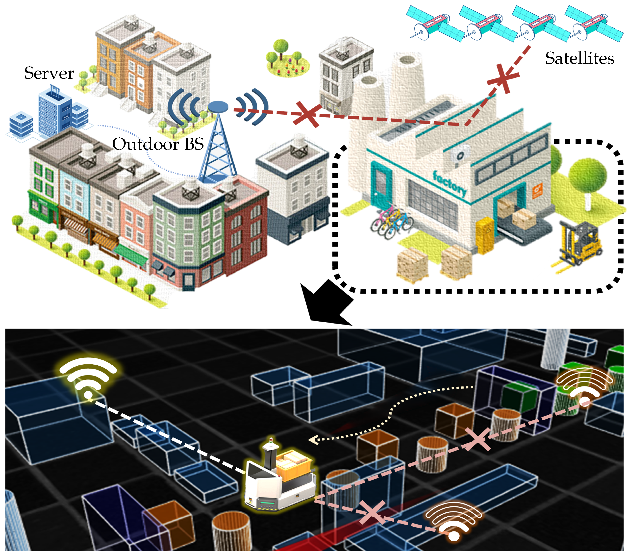
Taking a look at the evolution of modern localization techniques, the advancements in multiple-input multiple-output (MIMO) and multi-carrier technologies make great contributions. Localization techniques have expanded their capabilities by leveraging additional measurements on angle of arrival (AoA)- and time of arrival (ToA)-related information. This evolution has resulted in enhanced performance and better localization outcomes. Traditional wireless localization techniques often rely on triangulation or trilateration methods, which require three or more anchor points to perform the algorithm. However, in complex industrial environments, ensuring stable connections between multiple BS inherently introduces uncertainty. Moreover, unstable links, such as non-line-of sight (NLOS) transmissions between anchor points and the target, pose challenging obstacles to localization accuracy that are difficult to overcome [10,11] (see Figure 1). Therefore, in environments like factories and warehouses, single BS-assisted localization can be considered as an effective solution. In particular, joint angle and delay estimation (JADE) stands out as a promising solution, as it reduces the involvement of base stations and minimizes localization overhead, making it an excellent fit for various smart industry applications [12,13].

Figure 1.
Illustration of the single BS-assisted JAEDE, compared with other outdoor (upper) and indoor (lower) localization techniques.
There have been a number of mature studies that utilize JADE for localization in 2D environments, such as MUSIC and estimation of single parameters via rotational invariance techniques (ESPRIT), which offer their unique advantages [12,14,15]. For instance, the ESPRIT-based method in [12] achieves a low computational cost by using the Hadamard product, but it requires parameter pairing after the estimation, which introduces extra errors to the performance. The MUSIC-based algorithm in [14] estimates AoA and ToA components with relatively low complexity, but low signal-to-noise ratio (SNR) and sampling rate are still challenging. Another MUSIC-inspired approach presented in [15] achieves satisfactory accuracy using a two-step coarse and fine grid search. However, the fine search significantly increases the computational overhead.
All of the aforementioned works consider only 2D scenarios, while for 3D contexts, the addition of an extra dimension in 3D localization introduces an additional parameter that needs to be estimated, increasing the complexity of the localization process. This, in turn, leads to higher computational complexity and resource requirements. Another major challenge arises from the design of the antenna array. In 2D scenarios, a linear array configuration may suffice. However, in 3D environments, the array geometry must be more elaborate to capture the necessary spatial diversity for accurate AoA estimation. In [16,17], the UCA has already been utilized to estimate azimuth and elevation angle of arrival (AoA) jointly. They investigated the AoA estimation by MUSIC utilizing a uniform circular array (UCA), but they did not consider the ToA estimation at the same time.
In our previous publication [18], we have also proposed a single portable BS-assisted localization technique based on MUSIC for smart security scenarios. Our focus was on mitigating the computational burden associated with grid searching of the MUSIC algorithm and addressing the subsequent grid bias issues. However, there are several significant distinctions between our previous work and the current study. Firstly, our prior work primarily concentrated on 2D scenarios, limiting its ability to accurately estimate the vertical dimension or height of the target. Consequently, this limitation rendered it unsuitable for applications requiring localization in multiple vertical layers, such as warehouses. In contrast, the present study represents a notable advancement as we have expanded our methodology from 2D to 3D, together with a comprehensive evaluation of the performance of single BS-assisted localization techniques from various perspectives. This expansion sheds light on the unique challenges and potential solutions associated with 3D localization. Secondly, to accommodate the additional spatial dimension and the consequent performance challenges, we have upgraded our antenna model from a uniform linear array (ULA) to a UCA. This enhancement is a considerable improvement that addresses the new complexities introduced by the inclusion of the third dimension. By undertaking these enhancements and modifications, our current work substantially surpasses the limitations of our previous research, offering a more comprehensive and robust approach to 3D single BS-assisted localization techniques.
Table 1 summarizes all the aforementioned related works. Generally, the majority of current JADE algorithms encounter the issue of grid constraints. This means that during the search process, the estimated results are restricted to grid points. As a result, if the true values are off-grid, bias will persist regardless of the grid resolution. Unfortunately, the refinement process cannot be pushed to the extreme due to the resulting high computational complexity. Furthermore, studies concerning 3D environments are considerably fewer compared to those focusing on 2D scenarios, but the disparity between JAEDE and JADE cannot be ignored, since it is capable of providing accurate representation, enhancing spatial awareness, enabling safety and risk assessment, and optimizing performance.

Table 1.
Summary of Related Works.
Motivated by the aforementioned issues, we present a novel and computationally efficient localization technique for 3D IIoT scenarios. Our approach relies on a single BS and utilizes the MUSIC algorithm to estimate AoAz, AoAe, and ToA jointly. The key contributions of our work are as follows:
- We propose a localization algorithm that addresses the challenges of stable connectivity to multiple access points (AP) in IIoT scenarios, offering flexibility, easy implementation, and reduced computational cost compared to conventional multi-BS [19,20,21] and MUSIC-based single-BS [15] algorithms.
- To enhance performance without extensive grid searching, our algorithm incorporates Taylor-series in the iterative process, achieving a significant reduction in computational complexity with slight improvements in localization accuracy compared to a two-step MUSIC-based algorithm [15].
- Through numerical simulations, we compare our algorithm with three others, including MUSIC-based joint or separate angle and delay estimation. The results demonstrate that our algorithm consistently outperforms the alternatives in terms of AoAz, AoAe, ToA, and the overall location estimation accuracy across various SNR conditions.
Throughout the paper, capital boldface letters denote matrices; lowercase boldface letters denote vectors, e.g., stands for a complex matrix of the dimension ; is the identity matrix; stands for transposition; is the expectation; and represents the real part of a complex number.
2. System Model
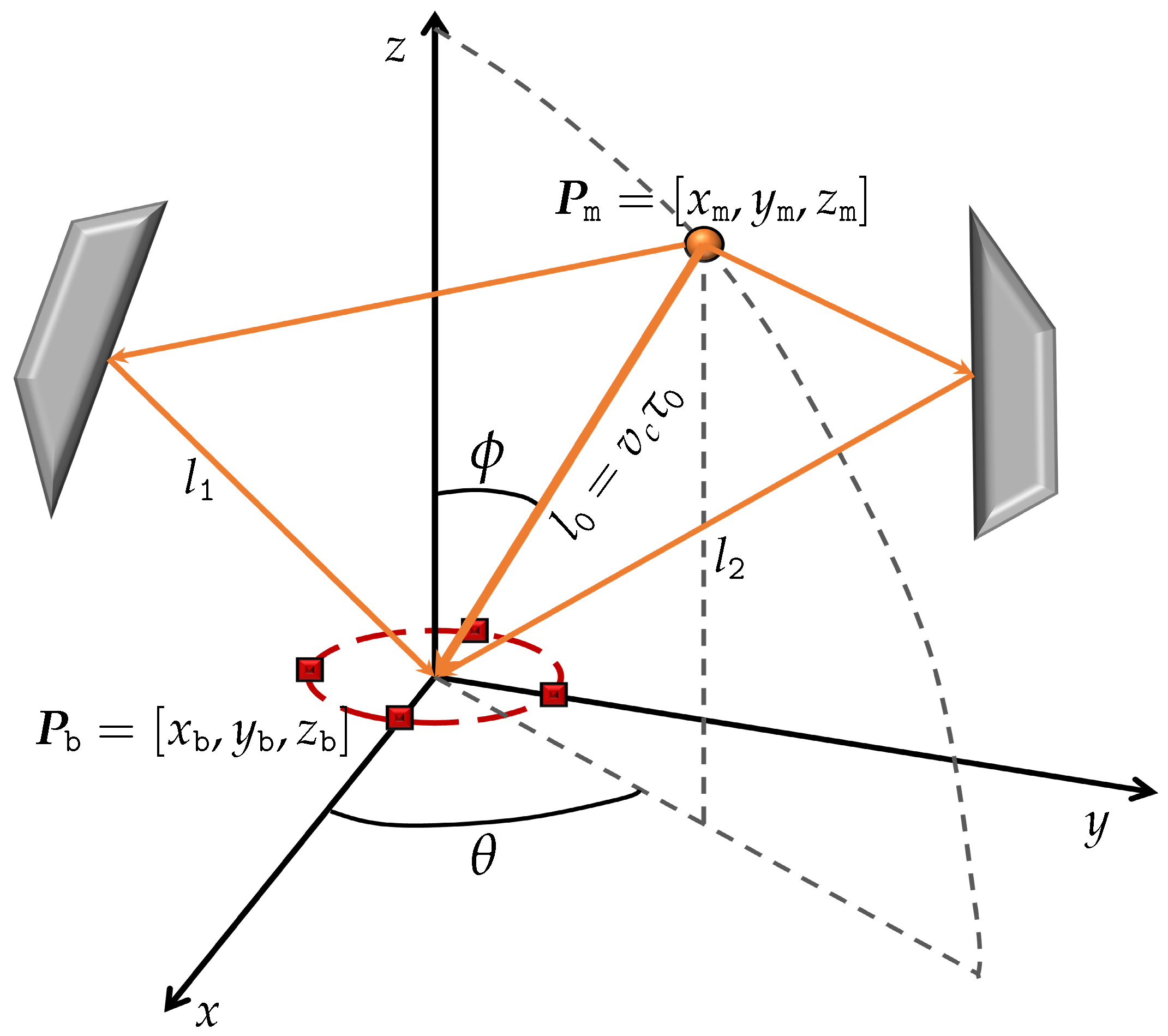
The JAEDE localization method introduces the system model as the basis of our approach. As depicted in Figure 2, the model consists of a mobile station (MS) located in a 3D Cartesian coordinate system at an unknown position denoted as . Communication between the MS and the BS involves a set of UCA positioned at a known location marked as . The main objective of the BS is to estimate the AoAz, AoAe, and ToA of the modulated signals transmitted from the MS, thereby enabling estimation of the MS’s coordinates. In accordance with our proposed approach, we consider the MS to be positioned at a far-field distance from the BS to maintain the generality of our framework.

Figure 2.
The 3D coordinate system, in which the propagation model is demonstrated with one MS (the orange ball) and three propagation paths to the UCA mounted on a BS at the origin.
In the analysis, we account for components contributing to multipath propagation. These components consist of a single line-of-sight (LOS) path with a length of , as well as NLOS paths, namely . The -th path, where , is characterized by its AoAz, AoAe, and ToA represented by , , and , respectively. Notably, we express , where m/s signifies the speed of light.
Assuming the UCA consists of identical sensor elements arranged equidistantly along a circle with a radius of r meters. The circle is positioned in the -plane of a local coordinate system, where the origin coincides with the center of the circle. In the coordinate system model represented in Figure 2, the azimuth angle, denoted as , is defined as the angle within the -plane, starting from the x-axis and pointing towards the y-axis. The elevation angle, denoted as , is defined as the angle starting from the -plane and moving towards the z-axis. The angular separation between any two adjacent elements within the array is . Consequently, the phase difference between the -th element and the origin can be expressed as , where , and represents the wavelength of the signal.
Given a transmitted signal , the received signal on the -th element of the UCA can be expressed as
where represents the complex attenuation of the -th multi-path component, with denoting the phase, and representing the additive white Gaussian noise (AWGN) on the -th array element. In addition, we perform the discrete Fourier transform (DFT) of the signal and consider sub-carriers with equal frequency increments. Consequently, the received sequence on the -th array element and the -th sub-carrier can be written as
where and are the corresponding channel frequency response and additive white Gaussian noise (AWGN), respectively. Considering the features of the AoAz, AoAe, and ToA of the UCA, the channel response yields
where is the sub-carrier frequency interval, and the channel gain.
Without loss of generality, we assume that the array elements of the UCA are identical and there is no mutual coupling or non-uniformity among them. Thus, for simplicity, we can normalize the gain in (3) [15]. Taking into account all the array elements of the Uniform Circular Array (UCA), sub-carriers, and multipath components, we can express (2) in matrix form as
with , . The steering matrix is formed from the steering element function:
The formation rule, as depicted in (6), shows only the indexes of within brackets, while omitting to simplify the notations. Now, we will introduce a three-step MUSIC-Taylor-based method to jointly estimate the AoAz, AoAe, and ToA using the steering matrix .
3. A Three Step MUSIC-Taylor-Based Localization Approach
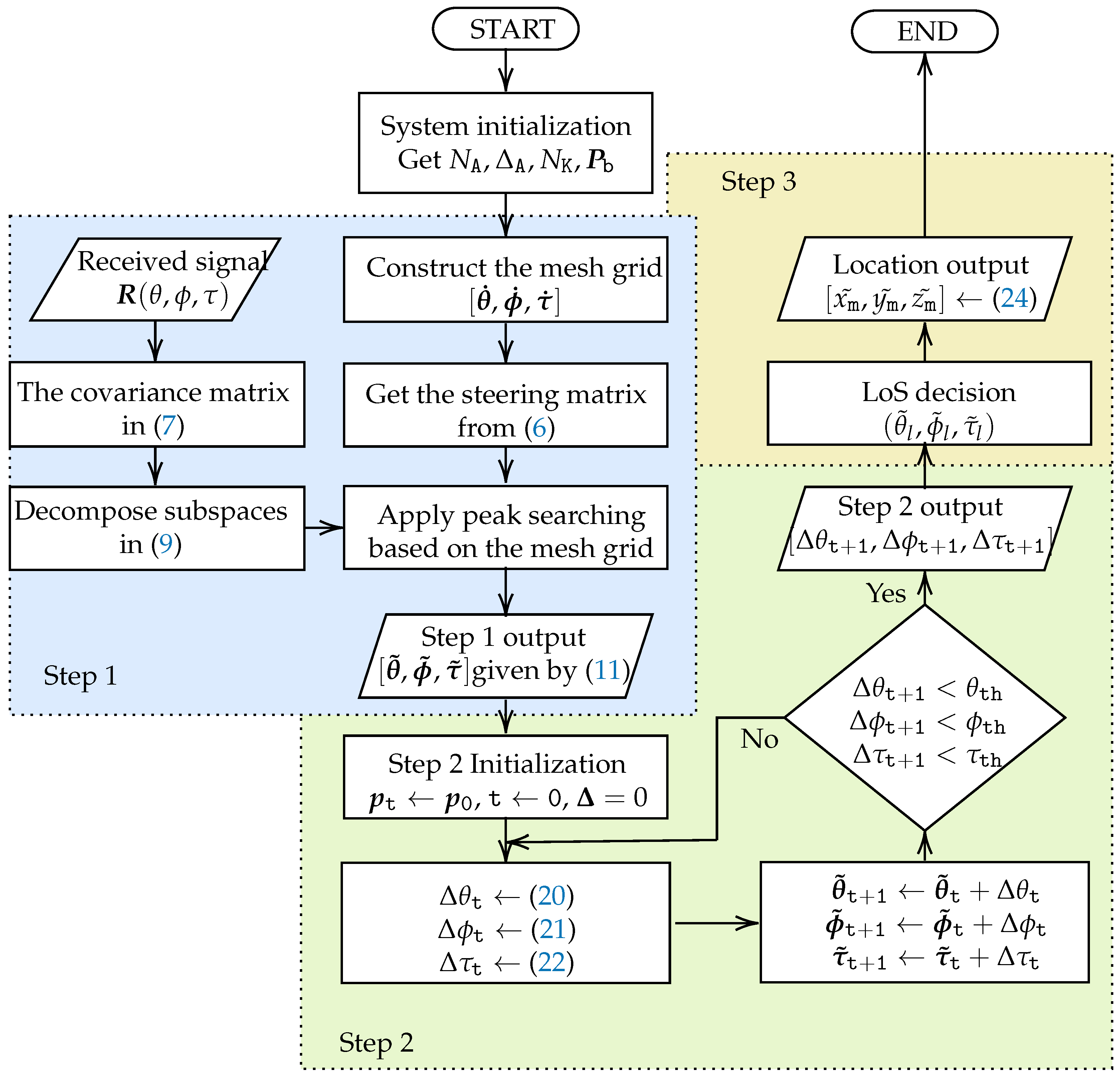
This section presents the proposed localization algorithm, which combines the MUSIC and Taylor-series techniques. The algorithm consists of three key steps: (1) Coarse localization using the MUSIC-based JAEDE algorithm; (2) Enhancement of the first step results using a Taylor-series-based approach, which helps mitigate the searching grid constraints introduced by the previous step; (3) Achieving precise localization with a single BS based on the estimated angles and delays obtained from the JAEDE process.
3.1. Step 1, MUSIC-Based Coarse JAEDE
The covariance matrix, , of the received signal, , in (4) is given by
Given that the noise is assumed to be a white Gaussian process with zero mean and variance , i.e., , and that it is independent among both the array elements and the signal, we can simplify the covariance matrix as follows:
where and are the covariance matrix of the signal and the noise, respectively. Additionally, let and represent diagonal matrices consisting of the eigenvalues of and , respectively. Given this, the covariance matrix can be decomposed as follows:
where, and denote the signal and noise subspaces, respectively. It is important to note that contains the top eigenvalues, while the remaining eigenvalues are included in . Since MUSIC-based approaches concentrate solely on the noise subspace, in the subsequent discussion, refers to unless specified otherwise. Consequently, the spectral function can be formulated as follows:
Since these two subspaces are orthogonal, the JAEDE results can be determined by the following object function,
where the vector of the estimated AoAz, AoAe and ToA correspond to the multipath components, and formed by , , and .
One approach commonly used for obtaining the pseudo-spectrum is grid searching. This involves constructing a three-dimensional mesh grid, , which divides the predefined range of AoAz (), AoAe (), and ToA () with equal spacing. The accuracy and complexity of the estimation depend on the number of grid points and the spacing between them. A smaller number of grids with larger spacing results in lower complexity but may lead to poorer accuracy. Therefore, in the initial stage, a coarse estimation is performed for computational efficiency. Later, an enhancement approach based on the Taylor-series is introduced to improve the estimation accuracy while maintaining low complexity. A summarized step-by-step implementation of Step 1, MUSIC-based coarse JAEDE is shown in Line 1 to 7, Algorithm 1.
| Algorithm 1 MUSIC-Taylor-based Single BS Localization |
3.2. Step 2, Taylor-Series Based Enhancement
Consider one of the points estimated in the previous MUSIC-based step, denoted as . Let represent the difference between this initial point and the true values, given by . The three-dimensional first-order Taylor-series expansion of the steering function around this initial point can be expressed as:
where , and are the first derivative with respect to , and , respectively. By substituting Equations (6), (11) and (12) into (10), the object function can be rewritten as a function of and ,
If is continuous, the minimization can be achieved by taking the first derivatives of (12) with respect to . To simplify the notation, we will omit the estimated point as variables, and also omit the subscript ‘’ in the following equations. Let represent the object function in Equation (13), denote the derivative , denote the derivative , and denote the derivative . The first-order partial derivatives of the object function in (13) with respect to , , and can be expressed as:
, , and can be solved by combining the linear functions (14)–(16), which can be written in determinant forms as,
Consequently, , , and of this iteration can be solved by the augmented matrix, and expressed in (20)–(22). Details of derivation can be found in Appendix A.
After obtaining the values of , , and , these values can be used to calculate the new pair of estimated points in the next iteration. Let the iteration begin with the point . Assuming that represents the current state, the current steering function can be obtained by replacing with in Equation (12). Consequently, , , and can be calculated step-by-step. Therefore, the estimation of the next state is given by:
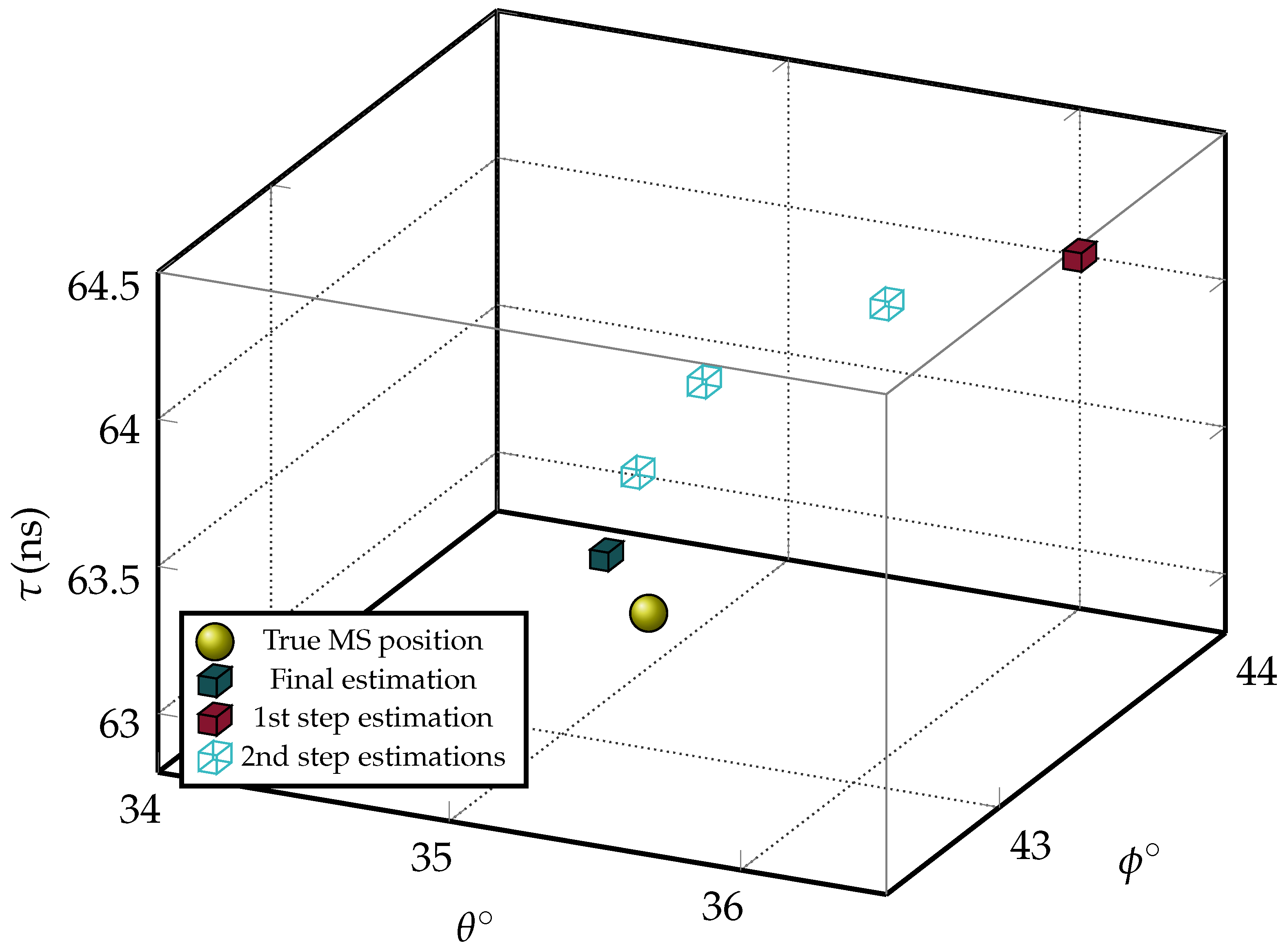
Figure 3 illustrates a simplified demonstration of the enhancement process for grid bias reduction through iterations. The ball represents the ground truth position of the target MS. The initial coarse estimation falls on the grid point at coordinates , where the grid constraints (i.e., the distance between the coarse estimation and the ground truth) are observable. The proposed Taylor-series-based enhancement method is then applied, which effectively eliminates the mis-distance through iterations. Please note that the figure provides a condensed view of the iterative process, and the actual simulation may involve denser iteration results. If the maximum number of iterations reaches or is less than a predefined threshold , the iteration will come to the end. The summarized implementation of the Taylor-series-based refinement can be found in lines 8 to 20 of Algorithm 1.
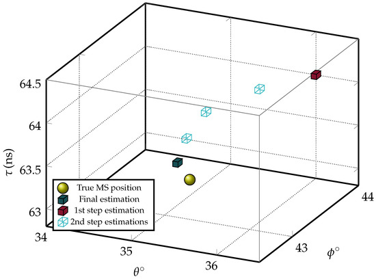
Figure 3.
A demo of the Step 1 coarse estimation, and Step 2 enhancement process.
3.3. JAEDE-Based Localization
In the final step of localizing the target MS using a single BS, the output AoAz, AoAE, and ToA are utilized. Among all the multipath components, it is highly likely that the path with the lowest time delay corresponds to the LOS path. For exceptional cases, specialized methods such as the PEak TRacking Algorithm (PETRA) can be employed to distinguish the LOS path from the NLOS multipath clusters [22]. However, these methods are beyond the scope of this discussion. Let represent the estimated LOS AoAz, AoAe, and ToA, as illustrated in Figure 2. The coordinates of the MS can be estimated using the following expression:
Algorithm 1 and the flow chart in Figure 4 summarize the full proposed localization technique step-by-step.
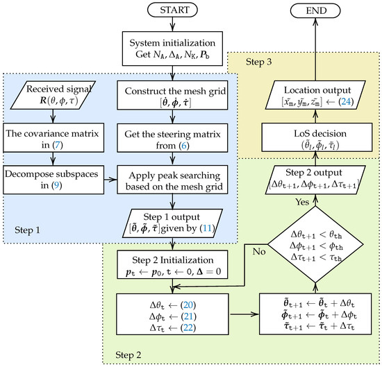
Figure 4.
Flow chart of the MUSIC-Taylor-based Single BS Localization algorithm.
It is important to note that the constraints of the algorithm should be considered when discussing the limitations and challenges faced in the proposed JAEDE approach. In this context, two key points can be highlighted. Firstly, accurate location estimation heavily depends on the determination of LOS. Any errors in LOS determination can significantly impact the accuracy of localization results. Therefore, improving LOS estimation techniques is essential for enhancing the overall performance of localization algorithms, particularly for IIoT scenarios where multipath effects can be severe. Secondly, the initial step of MUSIC-based coarse JAEDE acts as a crucial starting point that sets the stage for the entire algorithm, laying a robust foundation for its overall performance. The results of the first step should align closely with the grid points and be faithful to the available grid points, although grid spacing may be sparse. Otherwise, subsequent steps may not be able to effectively reduce the grid bias. There exists a performance bar for the Taylor expansion used in the second step, and surpassing this bar can be a potential direction for future research.
4. Performance Evaluation
In this section, the performance of the proposed localization algorithm is evaluated through Monte Carlo simulations, which take into account different SNR conditions and multipath activity patterns. The simulation parameters are detailed in Table 2, following a typical orthogonal frequency division multiplexing (OFDM) system setup. It is important to note that the coordinates of the MS should be calculated using the AoAz, AoAe, and ToA of the LOS path per Monte Carlo realization.
Table 2.
Simulation Parameters.
The performance is evaluated by the root mean square error (RMSE) metric averaged over multiple Monte Carlo realizations under different scenarios in terms of two major aspects, the accuracy of JAEDE estimation, and the mis-distance of the localization. For a given estimated result under one realization and the corresponding ground truth , with runs of Monte Carlo realizations, the RMSE is given by
where the operator (the norm) when the case is with regard to the location evaluation, and with the angle and delay estimation.
The performance of the proposed JAEDE-based localization technique (referred to as J-MT) is further compared with three other techniques:
- J-2M [15]: A two-step MUSIC-based algorithm, with coarse-fine grid spacing. In the following simulations, we extend the original 2D JADE method to 3D JAEDE, and choose coarse, find grid spacing of as and , respectively.
- S-MT: Using a MUSIC-Taylor algorithm similar to J-MT, but the angles and delay are estimated separately. The grid spacing for the 1st step MUSIC is the same as J-MT, .
- S-2M [15]: A two-step MUSIC-based algorithm, similar to J-2M, but the angles and delay are estimated separately, following the same grid spacing as J-2M.
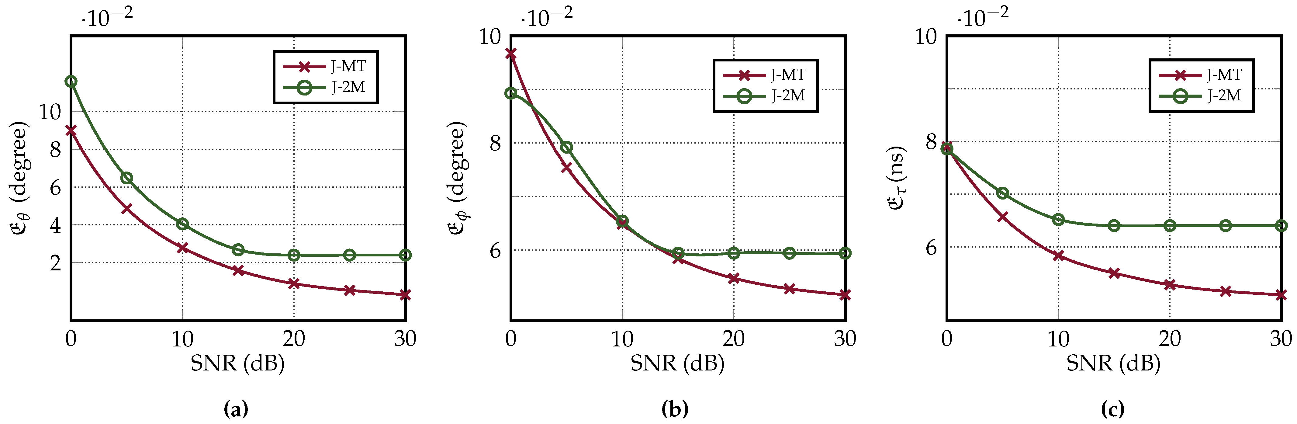
In the first comparison, we evaluate the performance of the proposed J-MT algorithm and compare it with a two-step classic MUSIC-based JAEDE algorithm called J-2M. The objective is to demonstrate the improvement achieved by reducing the grid constraints in the J-MT algorithm. The ground truth values for the three paths are deliberately set off-grid. Specifically, the AoAz, AoAe and ToA are , , and . As shown in Figure 5, the proposed J-MT method exhibits a stable downward trend. In terms of AoAz and ToA, the J-MT method consistently performs better than the J-2M method. In the case of AoAe, the J-MT method gradually outperforms the J-2M method as the SNR exceeds 15 dB. The slight upward tails of the J-2M method represent the performance limitation imposed by the grid constraints, which is effectively eliminated by the proposed J-MT method.

Figure 5.
The comparison on the grid bias elimination between J-MT and J-2M [15] for (a) AoAz, (b) AoAe, and (c) ToA estimation.
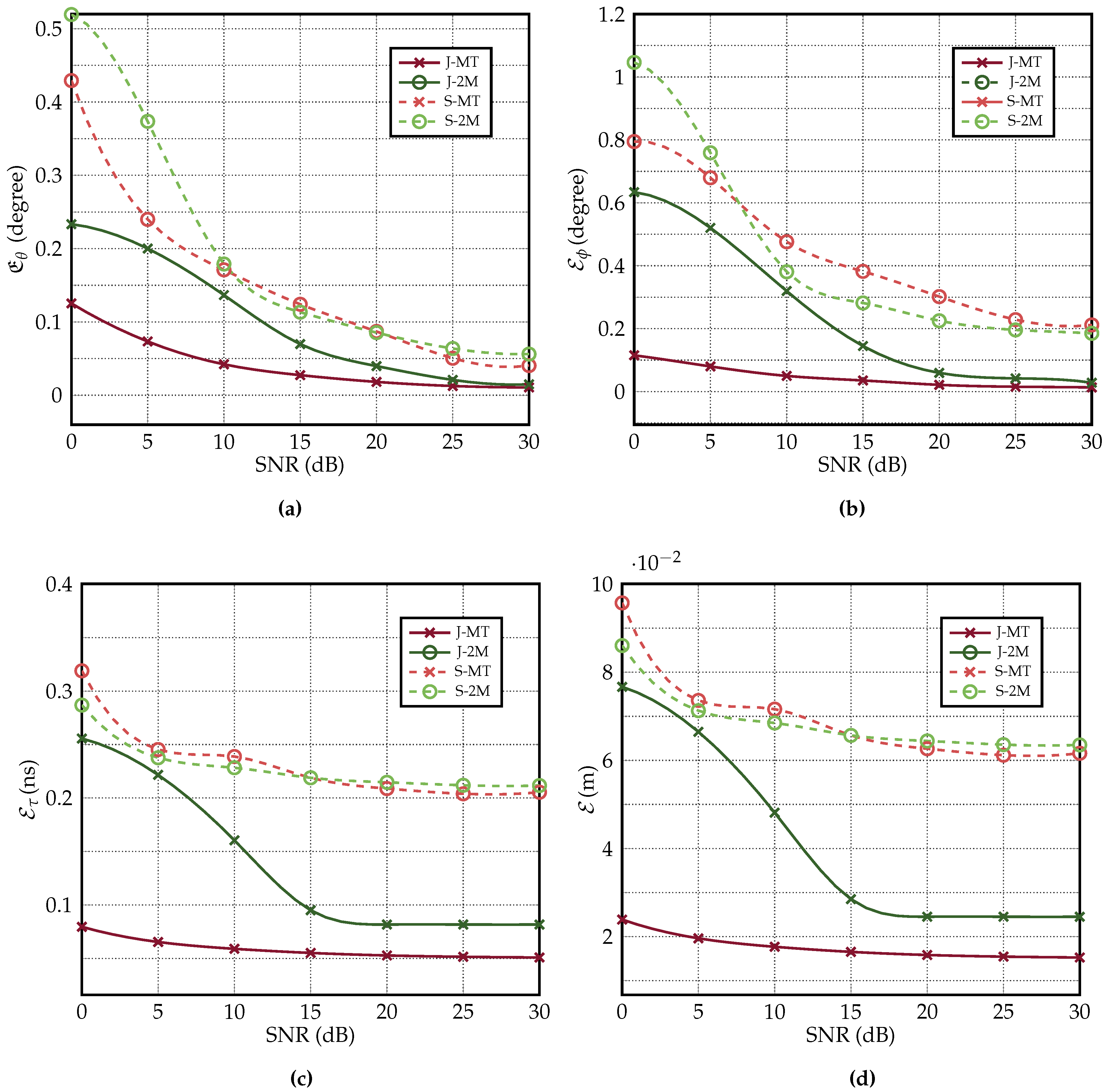
Figure 6 depicts the RMSE for the four candidate algorithms, with respect to AoAz, AoAe, ToA, and the overall location estimation under varying SNR conditions. To simulate the ground truth values of AoAz, AoAe, and ToA, we generate random variables distributed uniformly within a reasonable range, specifically, , , and ns. These ranges ensure that the MS is situated approximately 1 to 100 m away from the BS. Additionally, the minimum gap between any two components is set as 15 ns and (equal to three grid spacings), and any two paths closer than the minimum gap could be regarded as one cluster.
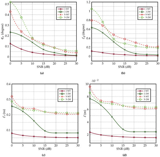
Figure 6.
Comparison of the (a) AoAz, (b) AoAe, (c) ToA, and (d) the overall location estimation performance under various SNR for J-MT, J-2M [15], S-MT, and S-2M.
Analyzing the sub-figures within Figure 6, we observe several common trends. As the SNR increases, all four algorithms consistently exhibit a decrease in RMSE, with the proposed J-MT method consistently outperforming the others. This highlights the superior performance of our proposed joint estimation approach. Moreover, the joint estimation methods (marked with ‘J’) consistently outperform the separate estimation methods (marked with ‘S’) in both angle and delay estimation. since the steering matrix adopted by the joint estimation takes advantage of both the antenna array and the sub-carrier frequency array, which is equivalent to an improvement in the antenna capability. Consequently, the joint estimation provided by the algorithms outperforms the separate estimation. However, it is noteworthy that the S-MT method does not exhibit significant superiority over the S-2M method. This limitation primarily arises from the initial MUSIC estimation. While the second-step Taylor enhancement can reduce estimation errors, its effectiveness is limited by the accuracy of the first step’s results. If the initial estimations deviate significantly from the ground truth, the second step may not fully compensate for those discrepancies. Additionally, the estimation of AoAz consistently outperforms that of AoAe. This can be attributed to two reasons: Firstly, AoAz contributes more to the phase difference at different array elements of the UCA compared to AoAe; Secondly, the elevation angle spread only spans from 0 to 90 degrees, which is half the azimuth angle range, posing additional challenges to the algorithm resolution in our specific setup.
Using the estimation results of Aoaz, AoAe, and ToA, along with the LOS judgment principle mentioned earlier, the location of the MS can be calculated. Consequently, the RMSE of the localization is depicted in Figure 6d for the four different algorithms, considering various SNR conditions. As anticipated, the accuracy of localization follows a similar trend to the accuracy of AoAz, AoAe, and ToA estimation. Our proposed algorithm consistently outperforms the other methods across different SNR conditions.
The last part of the performance evaluation is the computational complexity analysis. We mainly focus on the two MUSIC-based JAEDE algorithms, J-MT and J-2M [15]. Let G denote the number of grid points. Specifically, for the grid number of the coarse estimation in the J-MT method; and and for the grid number of the two steps in the J-MM method. Thus, the computational complexity for J-MT is
and for J-2M,
Adopting the settings for Figure 5, and assuming the maximum iterations for J-MT (the worst case in our simulations), for one Monte Carlo realization, the computational complexity of J-MT () takes up only of MM-2D complexity ().
5. Conclusions
In this paper, we propose the J-MT localization algorithm for the IIoT, aiming to address the challenges of indoor positioning using a single BS. The proposed method leverages the benefits of MUSIC-based JAEDE to effectively estimate the angle of azimuth, elevation, and time delay of the target. Moreover, the proposed approach eliminates the grid constraints that arise from the grid peak searching of conventional MUSIC-based methods, employing the Taylor-series method with a notable reduction in computational cost compared to the conventional two-step coarse-find grid searching MUSIC method. This advancement not only enhances accuracy but also improves the efficiency of the overall localization process. The comprehensive numerical results obtained through simulations have demonstrated the superiority of our proposed algorithm across various SNR conditions. It consistently outperforms other existing methods, including both separate angle and delay estimation, and two-step joint MUSIC localization algorithms.
Although the J-MT algorithm is originally proposed for indoor IIoT scenarios, it can also serve as a valuable inspiration for outdoor non-terrestrial network (NTN) applications with appropriate enhancements in both the antenna array and the algorithm design. In NTN scenarios, the longer distances between the airborne BS and the target introduce new challenges that need to be addressed. Firstly, the antenna array design must be improved to achieve higher angular sensitivity, while also considering compact size and low energy consumption. This is necessary to ensure accurate localization performance over extended distances. Secondly, the mobility of the BS, such as unmanned aerial vehicles (UAVs), presents additional obstacles that must be overcome. These include addressing link robustness, handover mechanisms, and potential interferences. By incorporating these improvements, the J-MT algorithm can be effectively adapted for NTN environments, enabling accurate localization even over large outdoor areas.
Author Contributions
Conceptualization, Z.L. and X.Z.; methodology, Z.L.; software, Z.L.; validation, Z.L.; formal analysis, Z.L.; investigation, Z.L.; resources, Z.L.; data curation, Z.L.; writing—original draft preparation, Z.L.; writing—review and editing, Z.L. and X.Z.; visualization, Z.L.; supervision, X.Z.; project administration, X.Z.; funding acquisition, X.Z. All authors have read and agreed to the published version of the manuscript.
Funding
This research was funded in part by the National Natural Science Foundation of China under Grant 62171161; in part by the Guangdong Provincial Science and Technology Program under Grant 2022A0505050022; in part by the Guangdong Basic and Applied Basic Research Foundation under Grant 2022B1515120018; in part by the Shenzhen Science and Technology Program under Grants ZDSYS20210623091808025, KQTD20190929172545139 and GXWD 20220817133854003; in part by the HIT-HKUST Joint Laboratory of Wireless Deterministic Networks.
Institutional Review Board Statement
Not applicable.
Informed Consent Statement
Not applicable.
Data Availability Statement
Data can be obtained from the corresponding author upon reasonable request.
Conflicts of Interest
The authors declare no conflict of interest.
References
- Liu, A.; Huang, Z.; Li, M.; Wan, Y.; Li, W.; Han, T.X.; Liu, C.; Du, R.; Tan, D.K.P.; Lu, J.; et al. A survey on fundamental limits of integrated sensing and communication. IEEE Commun. Surv. Tutor. 2022, 24, 994–1034. [Google Scholar] [CrossRef]
- Liu, F.; Cui, Y.; Masouros, C.; Xu, J.; Han, T.X.; Eldar, Y.C.; Buzzi, S. Integrated sensing and communications: Toward dual-functional wireless networks for 6G and beyond. IEEE J. Sel. Areas Commun. 2022, 40, 1728–1767. [Google Scholar] [CrossRef]
- Lohan, E.S.; Koivisto, M.; Galinina, O.; Andreev, S.; Tolli, A.; Destino, G.; Costa, M.; Leppanen, K.; Koucheryavy, Y.; Valkama, M. Benefits of positioning-aided communication technology in high-frequency industrial IoT. IEEE Commun. Mag. 2018, 56, 142–148. [Google Scholar] [CrossRef]
- Oyekanlu, E.A.; Smith, A.C.; Thomas, W.P.; Mulroy, G.; Hitesh, D.; Ramsey, M.; Kuhn, D.J.; McGhinnis, J.D.; Buonavita, S.C.; Looper, N.A.; et al. A Review of recent advances in automated guided vehicle technologies: Integration challenges and research areas for 5G-based smart manufacturing applications. IEEE Access 2020, 8, 202312–202353. [Google Scholar] [CrossRef]
- Yan, T. Positioning of logistics and warehousing automated guided vehicle based on improved LSTM network. Int. J. Syst. Assur. Eng. Manag. 2021, 14, 509–518. [Google Scholar] [CrossRef]
- Xiao, J.; Zhou, Z.M.; Yi, Y.W.; Ni, L.M. A survey on wireless indoor localization from the device perspective. Acm Comput. Surv. 2016, 49, 1–30. [Google Scholar] [CrossRef]
- Li, C.T.; Cheng, J.C.P.; Chen, K.Y. Top 10 technologies for indoor positioning on construction sites. Autom. Constr. 2020, 118, 103309. [Google Scholar] [CrossRef]
- Pei, T.; Li, D.; Liu, J.; Kong, W. Orthogonal time frequency space modulation-part III: ISAC and potential applications. IEEE Trans. Ind. Electron. 2023, 70, 5615–5625. [Google Scholar] [CrossRef]
- Fu, J.; Cui, B.; Wang, N.; Liu, X. A distributed position-based routing algorithm in 3-D wireless industrial internet of things. IEEE Trans. Ind. Inform. 2019, 15, 5664–5673. [Google Scholar] [CrossRef]
- Conti, A.; Mazuelas, S.; Bartoletti, S.; Lindsey, W.C.; Win, M.Z. Soft information for localization-of-things. Proc. IEEE 2019, 107, 2240–2264. [Google Scholar] [CrossRef]
- Zhu, Y.; Yan, F.; Zhao, S.; Xing, S.; Shen, L. On improving the cooperative localization performance for IoT WSNs. Ad Hoc Netw. 2021, 118, 102504. [Google Scholar] [CrossRef]
- Li, H.; Zheng, N.; Song, X.; Tian, Y. Fast estimation method of space-time two-dimensional positioning parameters based on Hadamard product. Intl. J. Antennas Prop. 2018, 2018, 7306902. [Google Scholar] [CrossRef]
- Zhu, X.; Qu, W.; Qiu, T.; Zhao, L.; Atiquzzaman, M.; Wu, D.O. Indoor intelligent fingerprint-based localization: Principles, approaches and challenges. IEEE Commun. Surv. Tutor. 2020, 22, 2634–2657. [Google Scholar] [CrossRef]
- Wang, Y.Y.; Chen, J.T.; Fang, W.H. TST-MUSIC for joint DOA-delay estimation. IEEE Trans. Signal Process. 2001, 49, 721–729. [Google Scholar] [CrossRef]
- Chen, L.; Qi, W.; Liu, P.; Yuan, E.; Zhao, Y.; Ding, G. Low-complexity joint 2-D DOA and TOA estimation for multipath OFDM signals. IEEE Signal Process. Lett. 2019, 26, 1583–1587. [Google Scholar] [CrossRef]
- Amine, I.M.; Seddik, B. 2-D DOA estimation using MUSIC algorithm with uniform circular array. In Proceedings of the 4th IEEE International Colloquium on Information Science and Technology (CiSt), Tangier, Morocco, 24–26 October 2016; pp. 850–853. [Google Scholar]
- Ihedrane, M.A.; Bri, S. Direction of arrival using uniform circular array based on 2-D MUSIC algorithm. Indones. J. Electr. Eng. Comput. Sci. 2018, 12, 30–37. [Google Scholar] [CrossRef]
- Li, Z.; Zhu, X. A portable base station assisted localization with grid bias elimination. In Proceedings of the 2023 IEEE Wireless Communications and Networking Conference (WCNC), Glasgow, UK, 26–29 March 2023; pp. 1–6. [Google Scholar]
- Zafari, F.; Gkelias, A.; Leung, K.K. A survey of indoor localization systems and technologies. IEEE Commun. Surv. Tutor. 2019, 21, 2568–2599. [Google Scholar] [CrossRef]
- Guo, X.; Ansari, N.; Hu, F.; Shao, Y.; Elikplim, N.R.; Li, L. A survey on fusion-based indoor positioning. IEEE Commun. Surv. Tutor. 2020, 22, 566–594. [Google Scholar] [CrossRef]
- Li, Z.; Giorgetti, A.; Kandeepan, S. Multiple radio transmitter localization via UAV-based mapping. IEEE Trans. Veh. Technol. 2021, 70, 8811–8822. [Google Scholar] [CrossRef]
- Klukas, R.; Fattouche, M. Line-of-sight angle of arrival estimation in the outdoor multipath environment. IEEE Trans. Veh. Technol. 1998, 47, 342–351. [Google Scholar] [CrossRef]
Disclaimer/Publisher’s Note: The statements, opinions and data contained in all publications are solely those of the individual author(s) and contributor(s) and not of MDPI and/or the editor(s). MDPI and/or the editor(s) disclaim responsibility for any injury to people or property resulting from any ideas, methods, instructions or products referred to in the content. |
© 2023 by the authors. Licensee MDPI, Basel, Switzerland. This article is an open access article distributed under the terms and conditions of the Creative Commons Attribution (CC BY) license (https://creativecommons.org/licenses/by/4.0/).