Study on the Frontal Collision Safety of Trains Based on Collision Dynamics

Abstract

The high-speed collision issue brought on by railway vehicles’ intensive and high-speed operation has become a critical concern for operational safety. Therefore, it is necessary to research the high-speed collision problem of trains. Firstly, a train collision dynamic model suitable for higher collision velocities is established. This model includes a 38-degree-of-freedom (DOF) three-dimensional vehicle model and a three-layered vibrating fixed-track model. Corresponding mathematical models are developed for nonlinear factors such as wheel–rail contact, car–end contact, and coupler overload representation in the model. Then, the Train Collision State Score (TCSS) is proposed, enabling quantitative safety evaluation under different collision conditions. Finally, the influence of the energy-absorbing device’s initial attitude and leading car parameters on collisions is studied. The results indicate that initial vertical height difference and pitching angle significantly increase TCSS. As the force level of the energy-absorbing device of the leading car increases, the effects of two intermediate coupler overload states on TCSS show opposite trends.

1. Introduction

With the rapid development of rail transportation, rail vehicles are moving towards higher speeds and increased operational density. Train collisions have become an undeniable safety issue, resulting in significant casualties and property damage worldwide every year. In North America, high-speed collision cases with collision velocities exceeding 36 km/h account for 43% of all collision accidents in the past 20 years. Similarly, high-speed collision accidents caused by overspeeding in Europe make up approximately 25% [1,2]. Addressing the problem of high-speed collisions becomes a decisive factor in further advancing the passive safety of trains.

Regarding research methods, common approaches to study train collision issues include conducting experiments and developing train collision models for numerical simulation calculations. These models include finite-element-based train collision models and multibody-dynamics-based train collision models. Meanwhile, new approaches based on traditional methods and machine learning can effectively address model-specific crash response prediction [3].

Although collision experiments [4,5,6,7] may have limitations regarding cost effectiveness, repeatability, and operability, they are necessary for verifying structural durability, formulating and establishing collision safety regulations, and optimizing and validating numerical calculation models. In order to balance the advantages and disadvantages of the collision test, scholars have studied the scaled model, and the establishment of a suitable scaled model can well restore the collision responses of the full-size model [8,9,10,11].

Finite-element-based train collision models can be used to investigate the comprehensive collision response of trains in various scenarios, including frontal collisions [12], oblique collisions [13], rollovers [14], and collisions with the operating environment [15,16]. They enable dynamic impact simulations ranging from component-level to full-scale vehicle-level analysis [17,18,19,20,21]. However, they suffer from complex modelling and long computation times. On the other hand, multibody-dynamics-based train collision models, while unable to provide information on structural deformation and stress distribution during collisions, offer a simplified modelling process and faster computation speed. Therefore, they are suited for initial analysis and parameter optimization in the design phase of high-speed collisions.

In terms of model development, multibody-dynamics-based train collision models can be categorized into one-dimensional, two-dimensional, and three-dimensional models. Yuan Chengbiao [22] developed a longitudinal train collision dynamic model and verified the model’s accuracy in longitudinal response through finite element methods. They also proposed multiple energy management schemes to achieve optimal energy allocation. The one-dimensional collision dynamic model primarily considers vehicle acceleration and energy utilization and is used to study energy allocation schemes and optimization problems for trains. Dias et al. [23] earlier extended the one-dimensional model to establish a two-dimensional train collision dynamic model. Three-dimensional models fully capture various responses during train collisions, and their three-dimensional coupling relationships accurately describe the interdependencies of trains during collisions. Therefore, they have become the focus and hotspot of research among scholars. Ling et al. [24] developed a three-dimensional nonlinear dynamic model for the oblique collision between passenger trains and road freight vehicles at level crossings. Using geometric-based derailment evaluation criteria, they studied the influence of critical parameters such as collision velocity, freight car mass, and collision angle on train derailment behavior. Hou et al. [25] evaluated the derailment risk based on the wheelsets’ lateral and vertical relative displacement and investigated the train collision and derailment issues using a three-dimensional train–track coupled dynamic model. Zhou et al. [26,27] utilized the SIMPACK to establish a three-dimensional collision model for the city tram and analyzed the factors causing derailment in city tram collisions and the response of the city tram when it is laterally impacted by a car at level crossings.

Currently, research on low-speed collisions below 36 km/h using dynamic models is relatively extensive and comprehensive. The models for the vehicle–track system, integration algorithms, and other aspects are relatively mature. Nonlinear factors such as the wheel–rail relationship and the mathematical model of the coupler have also experienced further advancements. However, such problems as car–end contact and coupler overload have not been thoroughly investigated in high-speed collisions. This lack of research leads to poor accuracy at higher collision speeds. Based on these two aspects, this paper establishes a three-dimensional train collision dynamic model suitable for higher collision velocities.

2. Three-Dimensional Train Collision Dynamic Model

Based on the traditional three-dimensional collision dynamic model, a three-dimensional train collision dynamic model applicable to higher collision velocities was established, as shown in Figure 1, by considering the vehicle’s actual structure and the functioning mechanisms of its components during high-speed collision. To accurately describe the vehicle’s motion during a high-speed collision, a three-dimensional vehicle model with 38 DOF was developed, including one carbody, two bogie frames, and four wheelsets. The carbody and bogie frame possess six degrees of freedom (longitudinal, lateral, vertical, roll, pitch, and yaw), and the wheelsets have five degrees of freedom (longitudinal, lateral, vertical, roll, and yaw). The carbody is connected to the frames via secondary suspension, and the frames are connected to the wheelsets via primary suspension. The dynamic equation of the model is as follows:

$$\mathit{M}\ddot{\mathit{u}}+\mathit{C}\dot{\mathit{u}}+\mathit{K}\mathit{u}=\mathit{F}$$

(1)

where $\mathit{M}$, $\mathit{C}$, and $\mathit{K}$ represent the mass matrix, damping matrix, and stiffness matrix, respectively. $\mathit{u}$ and $\mathit{F}$ denote the displacement vector and force vector, respectively.

By organizing and analyzing the dynamic equations of the vehicle model, the mass matrix of the vehicle model and the displacement vector can be obtained by Equations (2) and (3), respectively. The stiffness matrix is a sparse matrix of size 38 × 38, as shown in

Table A1. The non-zero elements of the stiffness matrix.

Location	Value	Location	Value
(1,1)	$4k_{\mathrm{ssz}}$	(1,2) (1,3) (2,1) (3,1)	$-2k_{\mathrm{ssz}}$
(2,8) (8,2)	$2k_{\mathrm{ssz}}{l}_{\mathrm{cb}}$	(2,2) (3,3)	$4k_{\mathrm{psz}}+2k_{\mathrm{ssz}}$
(2,4) (2,5) (3,6) (3,7) (4,2) (5,2) (6,3) (7,3)	$-2k_{\mathrm{psz}}$	(3,8) (8,3)	$-2k_{\mathrm{ssz}}{l}_{\mathrm{cb}}$
(4,4) (5,5) (6,6) (7,7)	$2k_{\mathrm{psz}}$	(4,9) (6,10) (9,4) (10,6)	$2k_{\mathrm{psz}}{l}_{\mathrm{bg}}$
(5,9) (7,10) (9,5) (10,7)	$-2k_{\mathrm{psz}}{l}_{\mathrm{bg}}$	(8,8)	$\begin{array}{l}4k_{\mathrm{ssz}}{l}_{\mathrm{cb}}^2+4k_{\mathrm{ssx}}{h}_{\mathrm{cb}}^2+\\ 2k_{\mathrm{trx}}{h}_{\mathrm{trc}}^2\end{array}$
(8,9) (8,10)	$2k_{\mathrm{ssx}}{h}_{\mathrm{cb}}{h}_{\mathrm{bgs}}-k_{\mathrm{trx}}{h}_{\mathrm{trc}}{h}_{\mathrm{trb}}$	(8,11)	$4k_{\mathrm{ssx}}{h}_{\mathrm{cb}}+2k_{\mathrm{trx}}{h}_{\mathrm{trc}}$
(8,12) (8,13)	$-2k_{\mathrm{ssx}}{h}_{\mathrm{cb}}-k_{\mathrm{trx}}{h}_{\mathrm{trc}}$	(9,8) (10,8)	$-2k_{\mathrm{ssx}}{h}_{\mathrm{bgs}}{h}_{\mathrm{cb}}$
(9,9) (10,10)	$\begin{array}{l}4k_{\mathrm{psz}}{l}_{\mathrm{bg}}^2-2k_{\mathrm{ssx}}{h}_{\mathrm{bgs}}^2+\\ 4k_{\mathrm{psx}}{h}_{\mathrm{bgp}}^2\end{array}$	(9,11) (10,11)	$-2k_{\mathrm{ssx}}{h}_{\mathrm{bgs}}-k_{\mathrm{trx}}{h}_{\mathrm{trb}}$
(9,12) (10,13)	$\begin{array}{l}2k_{\mathrm{ssx}}{h}_{\mathrm{bgs}}+4k_{\mathrm{psx}}{h}_{\mathrm{bgp}}+\\ k_{\mathrm{trx}}{h}_{\mathrm{trb}}\end{array}$	(9,14) (9,15) (10,16) (10,17)	$-2k_{\mathrm{psx}}{h}_{\mathrm{bgp}}$
(9,25) (10,25)	$-k_{\mathrm{trx}}{h}_{\mathrm{trb}}{h}_{\mathrm{trc}}$	(9,26) (10,27)	$k_{\mathrm{trx}}{h}_{\mathrm{trb}}^2$
(11,8)	$4k_{\mathrm{ssx}}{h}_{\mathrm{cb}}$	(11,9) (11,10)	$2k_{\mathrm{ssx}}{h}_{\mathrm{bgs}}$
(11,11)	$4k_{\mathrm{ssx}}+2k_{\mathrm{trx}}$	(11,12) (11,13)	$-2k_{\mathrm{ssx}}-k_{\mathrm{trx}}$
(12,8) (13,8)	$-2k_{\mathrm{ssx}}{h}_{\mathrm{cb}}$	(12,9) (13,10)	$-2k_{\mathrm{ssx}}{h}_{\mathrm{bgs}}+4k_{\mathrm{psx}}{h}_{\mathrm{bgp}}$
(12,11) (13,11)	$-2k_{\mathrm{ssx}}$	(12,12) (13,13)	$2k_{\mathrm{ssx}}+4k_{\mathrm{psx}}$
(12,14) (12,15) (13,16) (13,17) (14,12) (15,12) (16,13) (17,13)	$-2k_{\mathrm{psx}}$	(14,9) (15,9) (16,10) (17,10)	$-2k_{\mathrm{psx}}{h}_{\mathrm{bgp}}$
(18,18)	$4k_{\mathrm{ssy}}$	(14,14) (15,15) (16,16) (17,17)	$2k_{\mathrm{psx}}$
(18,25) (25,18)	$-4k_{\mathrm{ssy}}{h}_{\mathrm{cb}}$	(18,19) (18,20) (19,18) (20,18)	$-2k_{\mathrm{ssy}}$
(19,21) (19,22) (20,23) (20,24) (21,19) (22,19) (23,20) (24,20)	$-2k_{\mathrm{psy}}$	(18,26) (18,27)	$-2k_{\mathrm{ssy}}{h}_{\mathrm{bgs}}$
(19,26) (20,27)	$2k_{\mathrm{ssy}}{h}_{\mathrm{bgs}}-4k_{\mathrm{psy}}{h}_{\mathrm{bgp}}$	(19,25) (20,25) (20,32) (25,19) (25,20)	$2k_{\mathrm{ssy}}{h}_{\mathrm{cb}}$
(19,19) (20,20)	$2k_{\mathrm{ssy}}+4k_{\mathrm{psy}}$	(19,32)	$-2k_{\mathrm{ssy}}{l}_{\mathrm{cb}}$
(21,26) (22,26) (23,27) (24,27)	$2k_{\mathrm{psy}}{h}_{\mathrm{bgp}}$	(21,21) (22,22) (23,23) (24,24)	$2k_{\mathrm{psy}}$
(22,33) (24,34)	$2k_{\mathrm{psy}}{l}_{\mathrm{bg}}$	(21,33) (23,34)	$-2k_{\mathrm{psy}}{l}_{\mathrm{bg}}$
(25,26) (25,27)	$\begin{array}{l}-2k_{\mathrm{ssz}}{d}_{\mathrm{ss}}^2+2k_{\mathrm{ssy}}{h}_{\mathrm{cb}}{h}_{\mathrm{bgs}}\\ -k_{\mathrm{ar}}\end{array}$	(25,25)	$4k_{\mathrm{ssz}}{d}_{\mathrm{ss}}^2+4k_{\mathrm{ssy}}{h}_{\mathrm{cb}}^2+2k_{\mathrm{ar}}$
(26,19)	$-2k_{\mathrm{ssy}}{h}_{\mathrm{bgs}}-4k_{\mathrm{psy}}{h}_{\mathrm{bgp}}$	(26,18)	$2k_{\mathrm{ssy}}{h}_{\mathrm{bgs}}$
(26,20) (26,21) (27,22) (27,23)	$2k_{\mathrm{psy}}{h}_{\mathrm{bgp}}$	(26,26) (27,27)	$\begin{array}{l}2k_{\mathrm{ssz}}{d}_{\mathrm{ss}}^2-2k_{\mathrm{ssy}}{h}_{\mathrm{bgs}}^2+\\ 4k_{\mathrm{psz}}{d}_{\mathrm{ps}}^2+k_{\mathrm{ar}}+4k_{\mathrm{psy}}{h}_{\mathrm{bgp}}^2\end{array}$
(26,32) (32,26)	$2k_{\mathrm{ssy}}{h}_{\mathrm{bgs}}{l}_{\mathrm{cb}}$	(26,25) (27,25)	$\begin{array}{l}-2k_{\mathrm{ssz}}{d}_{\mathrm{ss}}^2-2k_{\mathrm{ssy}}{h}_{\mathrm{bgs}}{h}_{\mathrm{cb}}\\ -k_{\mathrm{ar}}\end{array}$
(27,18)	$2k_{\mathrm{ssy}}{h}_{\mathrm{bgs}}$	(26,28) (26,29) (27,30) (27,31) (28,26) (29,26) (30,27) (31,27)	$-2k_{\mathrm{psz}}{d}_{\mathrm{ps}}^2$
(27,32) (32,27)	$-2k_{\mathrm{ssy}}{h}_{\mathrm{bgs}}{l}_{\mathrm{cb}}$	(27,20)	$-2k_{\mathrm{ssy}}{h}_{\mathrm{bgs}}-4k_{\mathrm{psy}}{h}_{\mathrm{bgp}}$
(32,19)	$-2k_{\mathrm{ssy}}{l}_{\mathrm{cb}}$	(28,28) (29,29) (30,30) (31,31)	$2k_{\mathrm{psz}}{d}_{\mathrm{ps}}^2$
(32,32)	$4k_{\mathrm{ssx}}{d}_{\mathrm{ss}}^2+4k_{\mathrm{ssy}}{l}_{\mathrm{cb}}^2$	(32,20)	$2k_{\mathrm{ssy}}{l}_{\mathrm{cb}}$
(35,33) (36,33) (37,34) (38,34)	$-2k_{\mathrm{psx}}{d}_{ps}^2$	(33,33) (34,34)	$\begin{array}{l}2k_{\mathrm{ssx}}{d}_{\mathrm{ss}}^2+4k_{\mathrm{psx}}{d}_{\mathrm{ps}}^2+\\ 4k_{\mathrm{psy}}{l}_{\mathrm{bg}}^2\end{array}$
(35,35) (36,36) (37,37) (38,38)	$2k_{\mathrm{psx}}{d}_{ps}^2$

where $k_{\mathrm{psx}}$, $k_{\mathrm{psy}}$, and $k_{\mathrm{psz}}$ represent the longitudinal, lateral, and vertical stiffness of the primary suspension, respectively. $k_{\mathrm{ssx}}$, $k_{\mathrm{ssy}}$, and $k_{\mathrm{ssz}}$ represent the longitudinal, lateral, and vertical stiffness of the secondary suspension, respectively. $k_{\mathrm{trx}}$ represents the longitudinal stiffness of the traction rod. $k_{\mathrm{ar}}$ represents the stiffness of the anti-roll rod. $l_{\mathrm{cb}}$ and $h_{\mathrm{cb}}$ represent the longitudinal and vertical distance between the secondary suspension and the center of gravity of the carbody, respectively. $l_{\mathrm{bg}}$ represents the longitudinal distance between the primary suspension and the center of gravity of the frame. $h_{\mathrm{bgs}}$ and $h_{\mathrm{bgp}}$ represent the vertical distance between the secondary and primary suspension and the center of gravity of the frame, respectively. $h_{\mathrm{trc}}$ and $h_{\mathrm{trb}}$ represent the vertical distance between the traction rod and the center of gravity of the carbody and frame, respectively. $d_{\mathrm{ss}}$ and $d_{\mathrm{ps}}$ represent half of the lateral distance of two secondary and primary suspensions, respectively.

. The stiffness terms in the stiffness matrix are replaced with damping terms to obtain the damping matrix.

$$\begin{array}{c}{\mathit{M}}_{\mathrm{v}}=\mathrm{diag}(m_{\mathrm{cb}},m_{\mathrm{bg}},m_{\mathrm{bg}},m_{\mathrm{w}},m_{\mathrm{w}},m_{\mathrm{w}},m_{\mathrm{w}},I_{\mathrm{cby}},I_{\mathrm{bgy}},I_{\mathrm{bgy}},m_{\mathrm{cb}},m_{\mathrm{bg}},m_{\mathrm{bg}},\\ \hspace{1em}\hspace{1em}\hspace{1em} m_{\mathrm{w}},m_{\mathrm{w}},m_{\mathrm{w}},m_{\mathrm{w}},m_{\mathrm{cb}},m_{\mathrm{bg}},m_{\mathrm{bg}},m_{\mathrm{w}},m_{\mathrm{w}},m_{\mathrm{w}},m_{\mathrm{w}},I_{\mathrm{cbx}},I_{\mathrm{bgx}},\\ \hspace{1em} I_{\mathrm{bgx}},I_{\mathrm{wx}},I_{\mathrm{wx}},I_{\mathrm{wx}},I_{\mathrm{wx}},I_{\mathrm{cbz}},I_{\mathrm{bgz}},I_{\mathrm{bgz}},I_{\mathrm{wz}},I_{\mathrm{wz}},I_{\mathrm{wz}},I_{\mathrm{wz}})\end{array}$$

(2)

where $m$ and $I$ are mass and moments of inertia, respectively. The subscripts cb, bg, and w denote the carbody, bogie frames, and wheelsets, respectively.

$$\begin{array}{ll}{u}_{\mathrm{v}}=& [z_{\mathrm{cb}},z_{\mathrm{bg}1},z_{\mathrm{bg}2},z_{\mathrm{w}1},z_{\mathrm{w}2}.z_{\mathrm{w}3},z_{\mathrm{w}4},{\beta }_{\mathrm{cb}},{\beta }_{\mathrm{bg}1},{\beta }_{\mathrm{bg}2},x_{\mathrm{cb}},x_{\mathrm{bg}1},x_{\mathrm{bg}2},x_{\mathrm{w}1},\\ & x_{\mathrm{w}2},x_{\mathrm{w}3},x_{\mathrm{w}4},y_{\mathrm{cb}},y_{\mathrm{bg}1},y_{\mathrm{bg}2},y_{\mathrm{w}1},y_{\mathrm{w}2},y_{\mathrm{w}3},y_{\mathrm{w}4},{\alpha }_{\mathrm{cb}},{\alpha }_{\mathrm{bg}1},{\alpha }_{\mathrm{bg}2},\\ & {\alpha }_{\mathrm{w}1},{\alpha }_{\mathrm{w}2},{\alpha }_{\mathrm{w}3},{\alpha }_{\mathrm{w}4},{\gamma }_{\mathrm{cb}},{\gamma }_{\mathrm{bg}1},{\gamma }_{\mathrm{bg}2},{\gamma }_{\mathrm{w}1},{\gamma }_{\mathrm{w}2},{\gamma }_{\mathrm{w}3},{\gamma }_{\mathrm{w}4}{]}^{\mathrm{T}}\end{array}$$

(3)

where z, β, x, y, α, and γ represent the longitudinal, lateral, vertical, roll, pitch, and yaw motion, respectively.

The track model utilizes a fixed-track model with a three-layer discrete elastic support. The rail is simplified as a finite-length Euler beam supported by continuous elastic point supports. Below, are the sleeper and ground, which form a three-layer vibration model using distributed spring–damper units. Compared to the moving track model, this model can more accurately simulate the wheel–rail interaction force after high-speed collisions. The rail and sleeper have translational degrees of freedom in the vertical and lateral directions. If $E$, $I$, $l$, $m_r$, $N_k$, $m_s$, and $n_s$ denote the elastic modulus of the rail, moments of inertia of the rail section, length of each section of the rail, rail mass, maximum mode order of vibration for the rail, sleeper mass, and sleeper number, respectively, according to the differential equation governing the Euler beam vibration, the mass matrix and stiffness matrix of the track model can be obtained as follows:

$${\mathit{M}}_{\mathrm{R}}=\left[\begin{array}{cc}{\mathit{M}}_{\mathrm{r}}& 0\\ 0& {\mathit{M}}_{\mathrm{s}}\end{array}\right],K_{\mathrm{R}}=\left[\begin{array}{cc}{K}_{\mathrm{r}}& 0\\ 0& K_{\mathrm{s}}\end{array}\right]$$

(4)

where ${\mathit{M}}_{\mathrm{r}}$ is the dimensional identity matrix of size $2N_k$, and ${\mathit{M}}_{\mathrm{s}}$ is a diagonal matrix of size $n_s$ with all $m_s$ values on the main diagonal. Additionally,

$${\mathit{K}}_{\mathrm{r}}=\left[\begin{array}{cc}\frac{E{I}_y{\pi }^4}{m_r{l}^4}\mathrm{diag}\left(1^4,2^4,\dots ,N_k^4\right)& 0\\ 0& \frac{E{I}_z{\pi }^4}{m_r{l}^4}\mathrm{diag}\left(1^4,2^4,\dots ,N_k^4\right)\end{array}\right],K_{\mathrm{s}}=\left[\begin{array}{cc}{K}_{\mathrm{sz}}& 0\\ 0& K_{\mathrm{sy}}\end{array}\right]$$

where ${\mathit{K}}_{\mathrm{sz}}$ is a diagonal matrix of size $n_s$ with all $2k_{\mathrm{rsz}}+k_{\mathrm{sgz}}$ values on the main diagonal, and ${\mathit{K}}_{\mathrm{sy}}$ is a diagonal matrix of size $n_s$ with all $2k_{\mathrm{rsy}}+k_{\mathrm{sgy}}$ values on the main diagonal. Similarly, replacing the stiffness term with the damping term yields the damping matrix of the track model.

The combination of the vehicle model and track model yields a coupled vehicle–track model. For calculating the train collision problem consisting of p vehicles, the mass matrix, stiffness matrix, and damping matrix of the entire model can be obtained as follows:

$$\{\begin{array}{l}M=\mathrm{diag}\left(M_{\mathrm{VR}1},M_{\mathrm{VR}2},\dots ,M_{\mathrm{VRp}}\right)\hfill \\ K=\mathrm{diag}\left(K_{\mathrm{VR}1},K_{\mathrm{VR}2},\dots ,K_{\mathrm{VRp}}\right)\hfill \\ C=\mathrm{diag}\left(C_{\mathrm{VR}1},C_{\mathrm{VR}2},\dots ,C_{\mathrm{VRp}}\right)\hfill \end{array}$$

(5)

The train collision dynamic problem is a multi-degree-of-freedom nonlinear second-order differential equation typically solved using numerical integration methods. Yang et al. [28] proposed a corrected explicit method of double time steps that balances computational speed and accuracy for solving the train collision dynamic problem. This algorithm surpasses most other methods in terms of computational accuracy and exhibits significant advantages in computational speed. Therefore, we chose it as the integration method in this study.

3. The Nonlinear Factors and Their Mathematical Models in a Multibody System

It is crucial to establish appropriate mathematical models for the various nonlinear factors in the train collision dynamic model, including wheel–rail contact, car–end contact, and coupler forces.

3.1. Mathematical Model for Wheel–Rail Contact

To calculate the wheel–rail force, it is necessary to determine the position of the contact points between the wheel and rail. The trail method assumes that the contact points corresponding to all rolling circles of the wheel can be connected to form a spatial curve, thus improving scanning efficiency. After obtaining the minimum vertical clearance between the wheel and rail using the trail method [29], the normal compression at the contact point can be determined:

$$\Delta Z_c=\frac{\Delta Z_{\min }}{\cos \left(\delta \pm \phi \right)}$$

(6)

where $\Delta Z_c$ represents the normal compression at the contact point. $\Delta Z_{\min }$ represents the minimum vertical clearance between the wheel and rail. $\delta$ represents the contact angle, and $\phi$ represents the wheelset lateral roll angle.

After obtaining the normal compression, the normal contact force between the wheel and rail can be determined using Hertz contact theory:

$$F_N={\left(\frac{\Delta Z_c}{G}\right)}^{\frac{3}{2}}$$

(7)

where $G$ is the wheel–rail contact constant.

Finally, the creep force can be calculated using Polach’s creep theory:

$$F_T=\{\begin{array}{l}0,\sqrt{{\xi }_x^2+{\xi }_y^2}=0\hfill \\ \frac{2\mu F_N}{\pi }\left(\frac{k_{\mathrm{A}}\epsilon }{1+{\left(k_{\mathrm{A}}\epsilon \right)}^2}+\arctan \left(k_{\mathrm{S}}\epsilon \right)\right),\sqrt{{\xi }_x^2+{\xi }_y^2}\ne 0\hfill \end{array}$$

(8)

$$\{\begin{array}{l}{F}_{Tx}=-F_T\frac{{\xi }_x}{{\xi }_c}\hfill \\ F_{Ty}=-\frac{F_T{\xi }_y+F_{ys}{\xi }_{sp}}{{\xi }_c}\hfill \end{array}$$

(9)

where $F_T$ is the resultant creep force. $F_{Tx}$ and $F_{Ty}$ are longitudinal and lateral creep force, respectively. $k_{\mathrm{A}}$ and $k_{\mathrm{S}}$ are creep model coefficients. ${\xi }_x$ and ${\xi }_y$ are longitudinal and lateral creep rate, respectively. ${\xi }_{sp}$ denotes spin creep rate. $F_{ys}$ represents the influence of spin creep rate on longitudinal and lateral directions.

3.2. Mathematical Model for Car–End Contact

When a high-speed collision occurs, insufficient energy absorption by the coupler and anti-climbing device can cause car–end contact. Establishing a simple and fast algorithm for car–end contact is crucial for solving high-speed collision problems. Luo et al. [30] proposed a geometry-based compliant contact model for solving contact problems between two polyhedral bodies, which was applied to the dynamic simulation of a space station manipulator. However, it mainly focuses on calculating solid polyhedra under small deformation contact conditions. For train collision problems, the carbody can be considered a hollow, thin-walled polyhedron predominated by longitudinal length. The original formula has been modified for applicability based on the relationship between deformation and load during longitudinal impact. The original method, originally used for contact calculation between two solid polyhedra, is adapted for calculating the hollow carbody by introducing a stiffness weakening coefficient. Meanwhile, the original formula only applies to situations involving small plastic deformation. A steady-state coefficient is introduced to characterize the features of the steady-state crush stage. With the introduction of the stiffness weakening coefficient and steady-state coefficient, the car–end contact force can be expressed as:

$$P=\{\begin{array}{l}\lambda \gamma \pi \frac{E}{2(1-{\nu }^2)}\frac{A}{\tau }x,0\le x<x_{\mathrm{t}1}\hfill \\ f_{\mathrm{Interp}}\left(x\right),x_{\mathrm{t}1}\le x\le x_{\mathrm{t}2}\hfill \\ \eta P_{\max },x>x_{\mathrm{t}2}\hfill \end{array}$$

(10)

where $\lambda$ is the stiffness weakening coefficient. $\eta$ is the steady-state coefficient. $\gamma$ is a case coefficient. a and b represent the elastic modulus and Poisson’s ratio of the materials for the colliding carbody, respectively. $A$ represents the geometry contact area. $\tau$ represents the shape coefficient. $x$ denotes the car–end compression deformation. $P_{\max }$ represents the peak force. $x_{\mathrm{t}1}$ and $x_{\mathrm{t}2}$ are transition points of contact force, and $f_{\mathrm{Interp}}\left(x\right)$ is the transition interpolation function for compression.

For ease of engineering applications, further research was conducted on the determination of shape coefficient, stiffness weakening coefficient, and steady-state coefficient based on the structural analysis of a representative high-speed train through geometric derivation and numerical simulations.

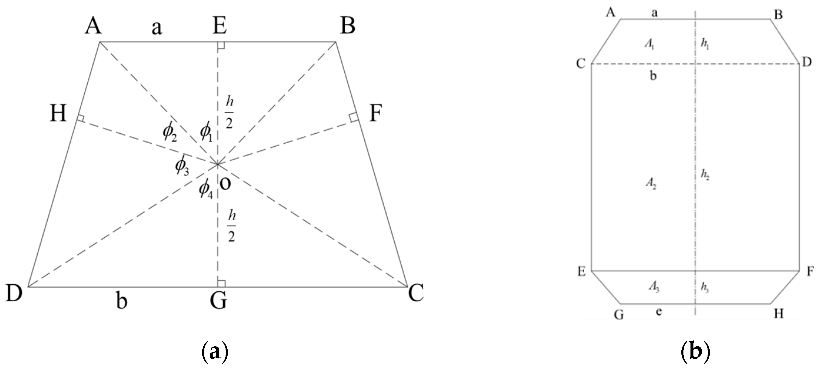
3.2.1. Shape Coefficient

An arbitrarily uniformly loaded polygon can be regarded as being composed of multiple right-angle triangles. A polygon with n sides can be divided into 2n right-angle triangles. Therefore, the shape coefficient of the section of any polygon can be calculated using Equation (11), as proposed in [31]:

$$\tau ={\displaystyle {\sum }_{i=1}^{2\mathrm{n}}{f}_i\frac{h_i}{2}\ln \left(\frac{1+\sin {\varphi }_i}{1-\sin {\varphi }_i}\right)}$$

(11)

where the value of $f_i$ takes either 1 or −1 based on the loading or unloading of the right-angle triangle. $h_i$ is the altitude of the right-angled triangle. ${\varphi }_i$ is the angle between two right-angle triangles.

The car ends of a typical high-speed train can be divided into the cab end and the intermediate car end. To facilitate calculations, the section of the crush zone can be geometrically simplified. The cab end section can be simplified as a symmetrical quadrilateral, while the intermediate car end section can be simplified as a symmetrical octagon. The simplified shapes and dimensional parameters of the section are shown in Figure 2.

By combining Equation (11) and Figure 2, the shape coefficient of the cab end can be calculated using the following equation:

$${\tau }_{cab}={\displaystyle \sum _{i=1}^4{h}_i\ln \left(\frac{1+\sin {\varphi }_i}{1-\sin {\varphi }_i}\right)}$$

(12)

where $h_1=h_4=\frac{h}{2}$, $h_2=h_3=\frac{ah+bh}{2\sqrt{{\left(b-a\right)}^2+h^2}}$, ${\varphi }_1=\arctan \frac{2a}{h}$, ${\varphi }_4=\arctan \frac{2b}{h}$, ${\varphi }_2=\arccos \frac{ah+bh}{\sqrt{{\left(b-a\right)}^2+h^2}\sqrt{4a^2+h^2}}$, ${\varphi }_3=\arccos \frac{ah+bh}{\sqrt{{\left(b-a\right)}^2+h^2}\sqrt{4b^2+h^2}}$.

The shape coefficient of the intermediate car end can be divided into three parts (A1, A2, and A3) and calculated separately, as shown in Equations (13)–(15):

$$\{\begin{array}{l}{\tau }_1=\frac{h_1}{2}\left(f_{\mathrm{SF}1}\left(\frac{2a}{h_1}\right)+f_{\mathrm{SF}1}\left(\frac{2b}{h_1}\right)\right)+Q_1\left(f_{\mathrm{SF}2}\left(W_1\right)+f_{\mathrm{SF}2}\left(E_1\right)\right)\hfill \\ {\tau }_2=h_2{f}_{\mathrm{SF}1}\left(\frac{2b}{h_2}\right)+2b{f}_{\mathrm{SF}1}\left(\frac{h_2}{2b}\right)\hfill \\ {\tau }_3=\frac{h_3}{2}\left(f_{\mathrm{SF}1}\left(\frac{2e}{h_3}\right)+f_{\mathrm{SF}1}\left(\frac{2b}{h_3}\right)\right)+Q_3\left(f_{\mathrm{SF}2}\left(W_3\right)+f_{\mathrm{SF}2}\left(E_3\right)\right)\hfill \end{array}$$

(13)

$$f_{\mathrm{SF}1}\left(x\right)=\ln \left(\frac{1+\sin \arctan x}{1-\sin \arctan x}\right),f_{\mathrm{SF}2}\left(x\right)=\ln \left(\frac{1+\sin \arccos x}{1-\sin \arccos x}\right)$$

(14)

$$\{\begin{array}{l}{Q}_1=\frac{\left(a+b\right)h_1}{2\sqrt{{\left(b-a\right)}^2+h_1{}^2}}\hfill \\ W_1=\frac{\left(a+b\right)h_1}{\sqrt{{\left(b-a\right)}^2+h_1{}^2}\sqrt{4b^2+h_1{}^2}}\hfill \\ E_1=\frac{\left(a+b\right)h_1}{\sqrt{{\left(b-a\right)}^2+h_1{}^2}\sqrt{4a^2+h_1{}^2}}\hfill \end{array},\{\begin{array}{l}{Q}_3=\frac{\left(e+b\right)h_3}{2\sqrt{{\left(b-e\right)}^2+{\left(h_3\right)}^2}}\hfill \\ W_3=\frac{\left(e+b\right)h_3}{\sqrt{{\left(b-e\right)}^2+h_3{}^2}\sqrt{4b^2+h_3{}^2}}\hfill \\ E_3=\frac{\left(e+b\right)h_3}{\sqrt{{\left(b-e\right)}^2+h_3{}^2}\sqrt{4e^2+h_3{}^2}}\hfill \end{array}$$

(15)

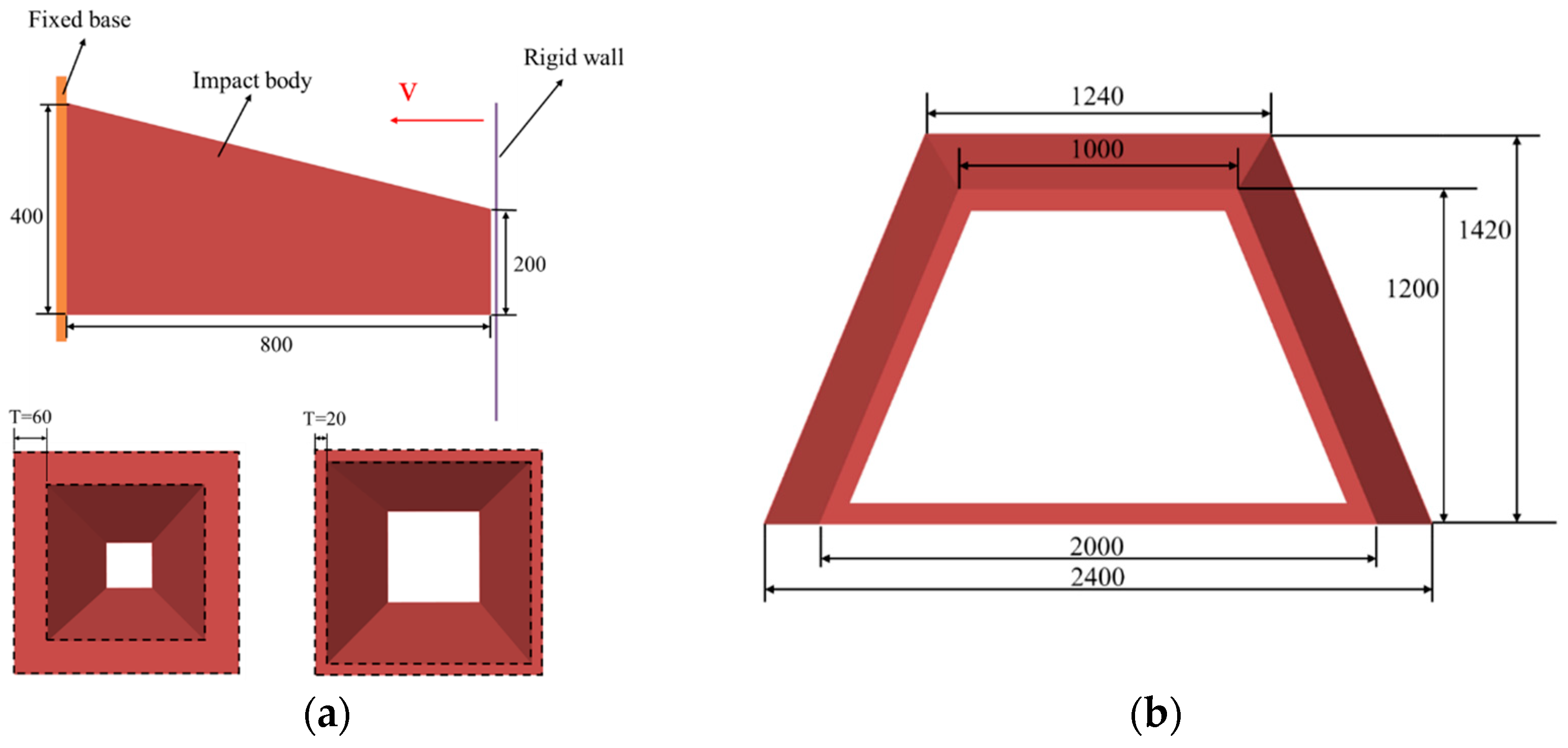
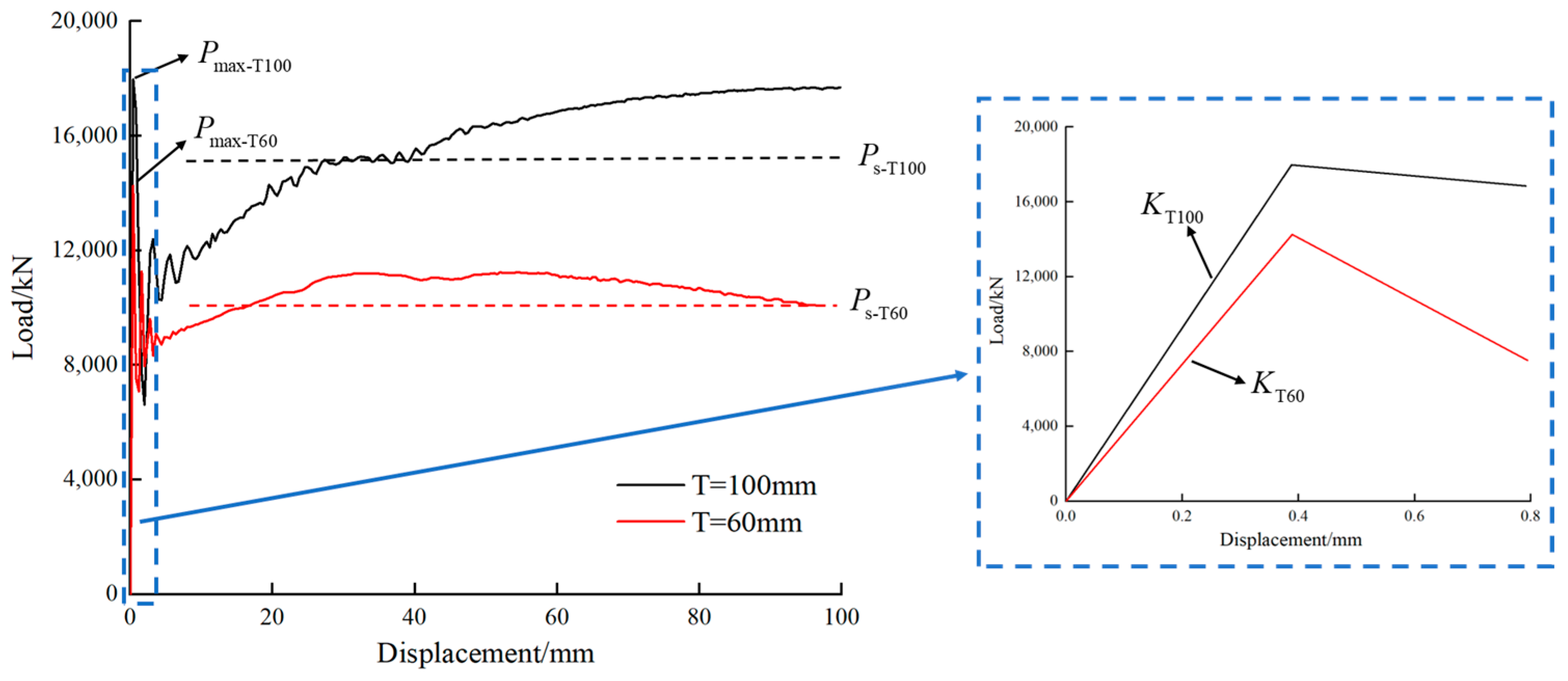
3.2.2. Stiffness Weakening Coefficient and Steady-State Coefficient

If the car–end crush zone of a high-speed train is simplified as a thin-walled, hollow polyhedron, the weakening law of the stiffness of the thin-walled, hollow polyhedron compared to its corresponding solid polyhedron, as well as the relationship between the volume ratio and the steady-state coefficient, can be established from the perspective of volume ratio. A finite element model was established in LS-DYNA, as shown in Figure 3a, to simulate the mechanical characteristics of the thin-walled structure after impact at different volume ratios. The model comprises a rigid wall, impact bodies with different volume ratios, and a fixed base. The fixed base and rigid wall are modelled using rigid material, while the impact bodies are modelled using elastic–plastic material. All components are modelled using solid elements. The simulation’s impact scenario involves a rigid wall with an initial velocity of 40 m/s impacting the aluminium alloy body with different volume ratios fixed on the base. The thin-walled body is a hexahedron with a square section. The side length of the front square section is 200 mm, the side length of the rear square section is 400 mm, and the overall length of the hexahedron is 800 mm.

To investigate the relationship between different volume ratios and the stiffness weakening coefficient and steady-state coefficient, finite element numerical simulations were conducted using various thicknesses of 100, 80, 60, 40, 20, 10, 5, and 1 mm. The simulations aimed to obtain the load–deformation relationship under dynamic impact conditions. The load–deformation relationship for the impact bodies with thicknesses of 100 mm (solid) and 60 mm subjected to impact loading from a rigid wall is shown in Figure 4.

After conducting multiple sets of numerical simulation experiments, the relationships between the stiffness weakening coefficient and steady-state coefficient with the volume ratio were obtained through polynomial fitting as follows:

$$\{\begin{array}{l}\lambda =-4.668Vo{l}_{\mathrm{r}}^6+13.523Vo{l}_{\mathrm{r}}^5-16.5Vo{l}_{\mathrm{r}}^4+8.829Vo{l}_{\mathrm{r}}^3-\\ \hspace{1em} 1.016Vo{l}_{\mathrm{r}}^2+0.828Vo{l}_{\mathrm{r}}+0.002\\ \eta =0.439Vo{l}_{\mathrm{r}}^4+0.629Vo{l}_{\mathrm{r}}^3-1.948Vo{l}_{\mathrm{r}}^2+1.294Vo{l}_{\mathrm{r}}+0.487\hfill \end{array}$$

(16)

where $Vo{l}_{\mathrm{r}}$ represents the volume ratio.

The obtained relationships are based on a specific model. To enhance their applicability, velocity and section variation factors are introduced to modify the stiffness weakening and steady-state coefficients. Assuming that there is no coupling relationship between the modification factors and no coupling relationship between the modification factors and the volume ratio, the individual effects of each modification factor on the stiffness weakening coefficient and the steady-state coefficient can be analyzed separately. Therefore, a thin-walled body with a volume ratio 0.24 was selected to study the modification factors.

The mechanical characteristics of the structure will exhibit significant differences under the impact of different velocities. Based on the original model, numerical experiments were conducted by varying the impact velocity with impact velocities set at 40, 35, 30, 25, 20, 15, and 10 m/s, respectively. It enabled the evaluation of the effects of different velocities on the two coefficients. After fitting the data, the relationship between the velocity modification factor and velocity can be obtained as follows:

$${\xi }_{\lambda }^v=0.896v_{\mathrm{r}}^3-2.721v_{\mathrm{r}}^2+2.841v_{\mathrm{r}}-0.015,{\xi }_{\eta }^v=\{\begin{array}{l}-3.36v_{\mathrm{r}}+2.49,v_{\mathrm{r}}<0.375\hfill \\ -v_{\mathrm{r}}+1.605,0.375\le v_{\mathrm{r}}<0.625\hfill \\ 1,v_{\mathrm{r}}\ge 0.625\hfill \end{array}$$

(17)

where ${\xi }_{\lambda }^v$ and ${\xi }_{\eta }^v$ represent the modification factor of stiffness weakening and steady-state coefficients, respectively. $v_{\mathrm{r}}$ denotes velocity ratio.

Due to variations in design, different trains may have different longitudinal sectional dimensions in their crush zones. Therefore, the section variation rate is introduced to characterize the influence of longitudinal sectional size variations on the two coefficients. The calculation of the section variation rate is given as follows:

$$SV=\frac{\sqrt{S_2}-\sqrt{S_1}}{l}$$

(18)

where $SV$ is the section variation rate. $S_1$ and $S_2$ are the front and rear section areas of the impact body, respectively. $l$ represents the length of the impact body.

The relationship between the section variation factor and the section variation rate was obtained through numerical simulations of eight scenarios where the section variation rates were 0, 0.1, 0.2, 0.25, 0.3, 0.4, 0.5, and 0.6, respectively, and where the volume ratio and the front section area were kept constant while the rear section area was varied. After fitting the data, the relationship between the section variation factor and the section variation rate is as follows:

$$\begin{array}{ccc}\begin{array}{l}{\xi }_{\lambda }^{SV}=0.068S{V}_{\mathrm{r}}^6-0.389S{V}_{\mathrm{r}}^5+0.793S{V}_{\mathrm{r}}^4-0.801S{V}_{\mathrm{r}}^3+\\ \hspace{1em}\hspace{1em} \hspace{0.17em}0.638S{V}_{\mathrm{r}}^2-0.007S{V}_{\mathrm{r}}+0.679\end{array}& ,& {\xi }_{\eta }^{SV}=\{\begin{array}{l}1.314,S{V}_{\mathrm{r}}=0\hfill \\ 1,S{V}_{\mathrm{r}}\ne 0\hfill \end{array}\end{array}$$

(19)

where ${\xi }_{\lambda }^{SV}$ and ${\xi }_{\eta }^{SV}$ are the section variation factor of the stiffness weakening coefficient and steady-state coefficient, respectively; $S{V}_{\mathrm{r}}$ denotes the ratio of section variation rate.

Based on the assumption of non-coupling, the modification factors for the stiffness weakening coefficient and the steady-state coefficient can be obtained as follows:

$${\xi }_{\lambda }={\xi }_{\lambda }^v\cdot {\xi }_{\lambda }^{SV},{\xi }_{\eta }={\xi }_{\eta }^v\cdot {\xi }_{\eta }^{SV}$$

(20)

To verify the accuracy of the application to different section shapes and the degree of coupling between the modification factors, a validation model with a volume ratio of 0.2 was designed, as shown in Figure 3b. Numerical simulations were conducted at an impact velocity of 28 m/s. The stiffness weakening and steady-state coefficients obtained through finite element numerical simulations and calculations are shown in

Table 1. Comparison between the fitting formula and finite element numerical simulation.

	Fitting Formula Value	Numerical Simulation Value	Relative Error
stiffness weakening coefficient	0.166	0.175	5.14%
steady state coefficient	0.673	0.714	5.74%

. This indicates good accuracy of the results with a relative error of approximately 5%.

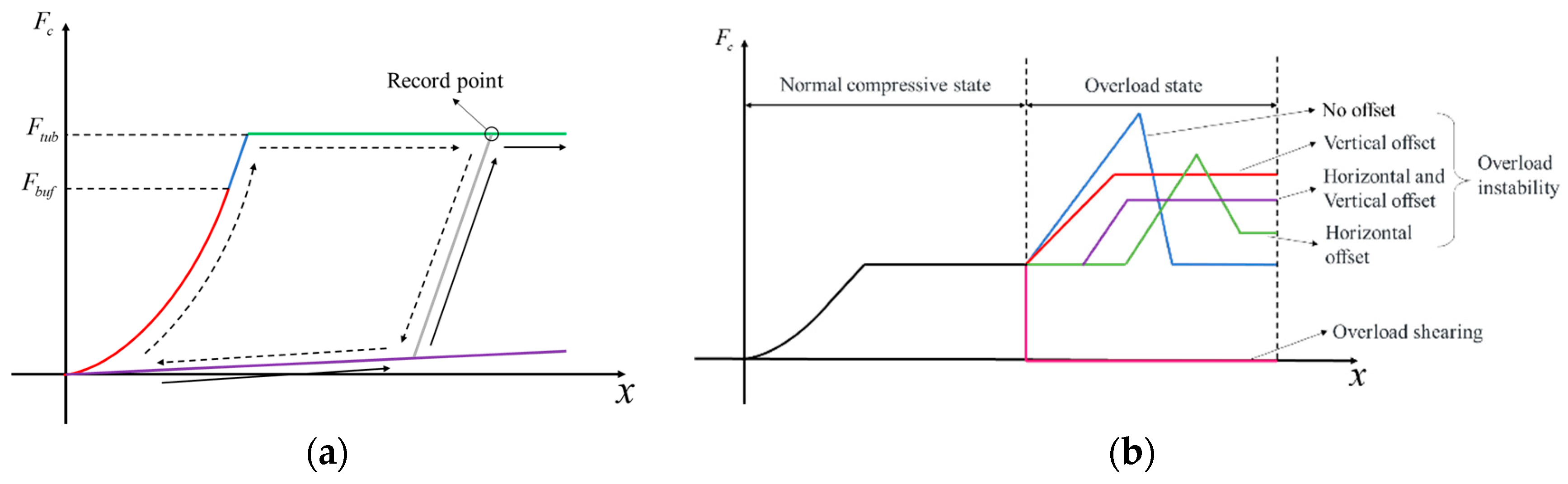
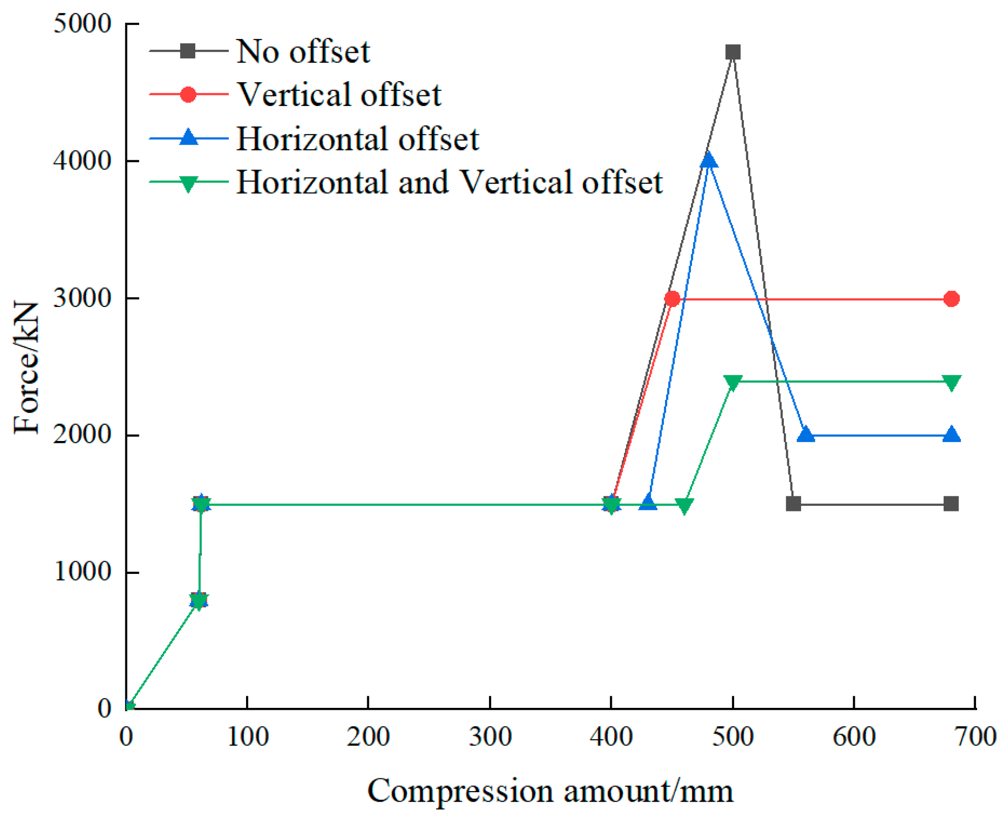
3.3. Mathematical Model for Coupler

The buffer and collapse tube of the coupler act sequentially during the collision compression process. To address the loading–unloading conversion caused by velocity changes during the collision process, a composite curve method is employed to construct the characteristic curve of the coupler. Figure 5a illustrates this curve, where the dashed arrow represents the path of the coupler’s initial loading and unloading, and the solid arrow represents the coupler’s secondary loading path. The red line is the buffer action stage, and the blue line is the transition stage that at this time the buffer reaches the limit load but has not yet reached the trigger load of the collapse tube. The green line is the collapse tube action stage, the purple line is the unloading stage of the buffer, and the gray line is the loading-unloading transition stage. The compression state of the coupler is recorded in real time by setting the maximum compression displacement $d_{\max }$ and maximum compression force $F_{\max }$. By constructing different transition curves using the maximum compression displacement, maximum compression force, and unloading curve of the buffer, the calculation of the coupler force becomes faster and more stable. This approach helps avoid oscillation issues that may arise during velocity changes. The coupler force during the collision compression process can be calculated using the following equation:

$$F_c(x)=\max \left(f_{lo}(x),f_{ut}(x)\right)$$

(21)

where $f_{lo}(x)$ represents the loading function of the coupler, and $f_{ut}(x)$ denotes the unloading transition function of the coupler.

When a high-speed collision occurs, the coupler may experience overload, meaning that the rated energy absorption capacity of the buffer and collapse tube cannot meet the energy absorption requirements during high-speed collisions. In traditional models, it is commonly assumed that the axial force of the intermediate coupler increases linearly with the compression displacement after overload. However, this assumption does not accurately reflect the actual behavior of the intermediate coupler. Zhang et al. [32] conducted a study on the collision characteristics of the intermediate coupler under deflection angle by developing an elaborate finite element model. The results showed that the intermediate coupler experiences instability after overload. By combining the compression characteristics of the intermediate coupler in its normal compressive state, a comprehensive representation model of the compression state throughout the collision process of the intermediate coupler can be obtained, as shown in Figure 5b.

3.4. Mathematical Model for Other Nonlinear Factors

There are also models for anti-climbing devices and stop devices in collision dynamics models. Anti-climbing devices are typically installed at the ends of trains and can absorb the remaining collision kinetic energy after the heading coupler has sheared off. The anti-climbing devices model is relatively mature, and their loading characteristics can be described as follows:

$$F_{alo}(x)=\{\begin{array}{l}0,x<d_g\hfill \\ k_a\left(x-d_s\right),d_g\le x<d_u+d_g\hfill \\ F_s,d_u+d_g\le x<d_g+d_u+d_s\hfill \\ F_s+k_a\left(x-d_g-d_u-d_s\right),x\ge d_g+d_u+d_s\hfill \end{array}$$

(22)

where $d_g$ represents the initial distance between two anti-climbing devices. $d_u$ represents deformation when the anti-climbing device reaches steady-state force. $d_s$ denotes the total stroke of the anti-climbing device. $k_a$ denotes the contact stiffness of the anti-climbing device, and $F_s$ denotes the steady-state force of the anti-climbing device.

Due to the lack of a buffer, the force of the anti-climbing device becomes zero directly after unloading. Similarly, the characteristic curve of the anti-climbing device during the collision process can be constructed. Common stop devices include secondary suspension lateral and vertical stop and primary suspension vertical stop. Their purpose is to limit significant relative displacement between the carbody and the frame and between the frame and the wheelset. In collision dynamics models, stop force is applied using stiffness, and its calculation method is as follows:

$$F_b\left(x\right)=\{\begin{array}{l}0,\left|x\right|<\delta \hfill \\ k_b\left(\left|x\right|-\delta \right)\mathrm{sgn}(x),\left|x\right|\ge \delta \hfill \end{array}$$

(23)

where $F_b\left(x\right)$ is stop force. $\delta$ represents stop clearance, and $k_b$ denotes stop stiffness.

4. Research on High-Speed Collision Safety of Trains and Results Analysis

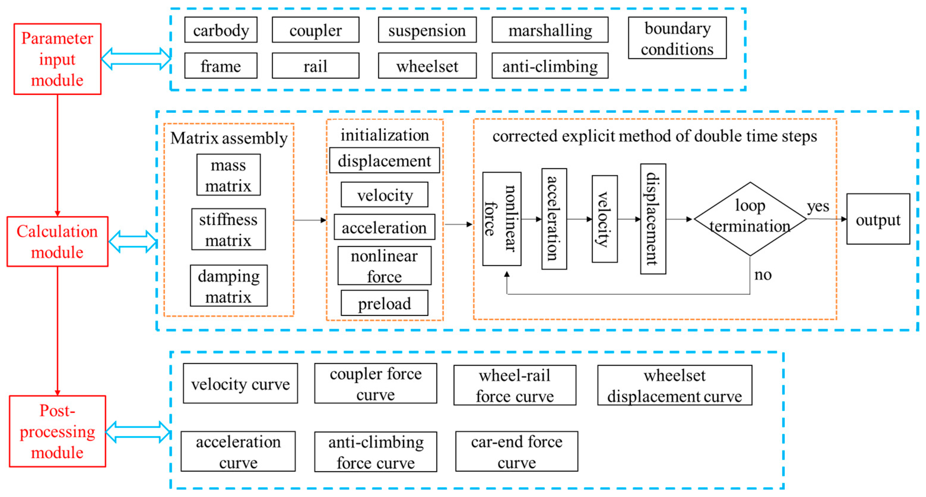
4.1. Dynamic Calculation Program and Collision Scenarios

A simulation calculation program using MATLAB based on the train collision dynamic mathematical model has been developed. The program consists of three main modules, as shown in Figure 6. These modules are the parameter input, calculation, and post-processing modules. They enable dynamic simulation calculations of frontal collisions for trains of any configuration at arbitrary velocities.

To conduct safety research on high-speed collisions, a collision scenario was set up where a moving four-unit trainset impacts a stationary train of the same configuration at a 48 km/h speed, as depicted in Figure 7. The inertia and suspension parameters of the vehicle can be found in

Table A2. The inertia parameters of the vehicle.

Component	Mass/ kg	X-Axis Moment of Inertia/ $\mathbf{kg}\cdot {\mathbf{m}}^2$	Y-Axis Moment of Inertia/ $\mathbf{kg}\cdot {\mathbf{m}}^2$	Z-Axis Moment of Inertia/ $\mathbf{kg}\cdot {\mathbf{m}}^2$
A1 carbody	35,542	82,867	1.68 × 106	1.69 × 106
A2 carbody	33,937	86,337	1.95 × 106	1.95 × 106
A3 carbody	33,937	86,337	1.95 × 106	1.95 × 106
A4 carbody	35,542	82,867	1.68 × 106	1.69 × 106
frame of power bogie	3671	2895	1838	4582
wheelset of power bogie	2177	1581	—	1607
frame of trailer bogie	2724	2148	1364	3399
wheelset of trailer bogie	1642	1192	—	1212

and

Table A3. The suspension parameters of the vehicle.

Component	Stiffness			Damping
	Vertical	Longitudinal	Lateral	Vertical	Lateral
primary suspension	1.25 × 106	1.10 × 108	5.70 × 106	9.80 × 103	9.80 × 103
secondary suspension	3.85 × 105	9.00 × 105	5.70 × 106	3.60 × 104	3.60 × 104
traction rod	-	1.58 × 108	-	-	-

. The parameters for the energy absorption devices of the vehicles are listed in

Table 2. Energy absorption devices parameters.

Device Name	Buffer		Collapse Tube		Shearing Force/ N	Contact Stiffness/ $\mathbf{N}\cdot {\mathbf{m}}^{-1}$
	Stiffness/ $\mathbf{N}\cdot {\mathbf{m}}^{-1}$	Stroke/ m	Stiffness/ $\mathbf{N}\cdot {\mathbf{m}}^{-1}$	Stroke/ m
heading coupler	1.00 × 107	0.10	1.50 × 106	1.30	1.55 × 106	-
intermediate coupler	1.33 × 107	0.06	1.50 × 106	0.34	1.55 × 106	-
anti-climbing	-	-	1.00 × 106	0.50	-	5.00 × 107
stop	-	-	-	-	-	1.00 × 107

, and the sectional parameters of the crush zone at the ends of the vehicles can be found in

Table 3. Geometric parameters of the crush zone at the ends of the vehicles.

Notation		Value	Notation		Value
cab end front section/ m	a1	0.57	intermediate end section/ m	a	1.08
	b1	0.96		b	1.58
	h1	0.91		e	1.15
cab end rear section/ m	a2	1.23		h1	0.81
	b2	1.62		h2	1.15
	h2	2.54		h3	0.91

. The intermediate coupler experiences two states after overload, instability and shearing, and the instability characteristic curve is depicted in Figure 8.

4.2. Assessment of Train Collision States

To quantitatively assess the safety of trains after high-speed collisions under different conditions, a Train Collision State Score (TCSS) has been established based on three evaluation indicators of crashworthiness according to the EN15227 standard. These indicators include wheel uplift displacement, car–end crush deformation, and the 30 ms maximum average acceleration. The Train Collision State Score (TCSS) is obtained by summing up the Vehicle State Scores (VSS) of the individual vehicles in a trainset. The calculation method for the VSM of a single vehicle is as follows.

Firstly, the calculation methods for each evaluation indicator are as shown in Equation (24):

$$Inde{x}_i=\frac{va{l}_{ic}-va{l}_{is}}{va{l}_{is}}$$

(24)

where $i=wl,\hspace{0.17em}cru,\hspace{0.17em}acc$ represent the wheel uplift displacement, car–end crush deformation, and 30 ms maximum average acceleration, respectively; $va{l}_{ic}$ and $va{l}_{is}$ represent the simulation calculated values and standard specified values of the evaluation indicators, respectively.

Then, by using the Analytic Hierarchy Process (AHP) to analyze the hierarchical relationships, the weight coefficients for the three evaluation indicators can be obtained. Subsequently, the calculations for VSS and TCSs can be expressed as follows, according to Equation (25):

$$\{\begin{array}{l}VSM=0.3956Inde{x}_{wl}+0.3297Inde{x}_{cru}+0.2747Inde{x}_{acc}\hfill \\ TCSM={\displaystyle \sum _{i=1}^{n}VS{M}_i}+10\hfill \end{array}$$

(25)

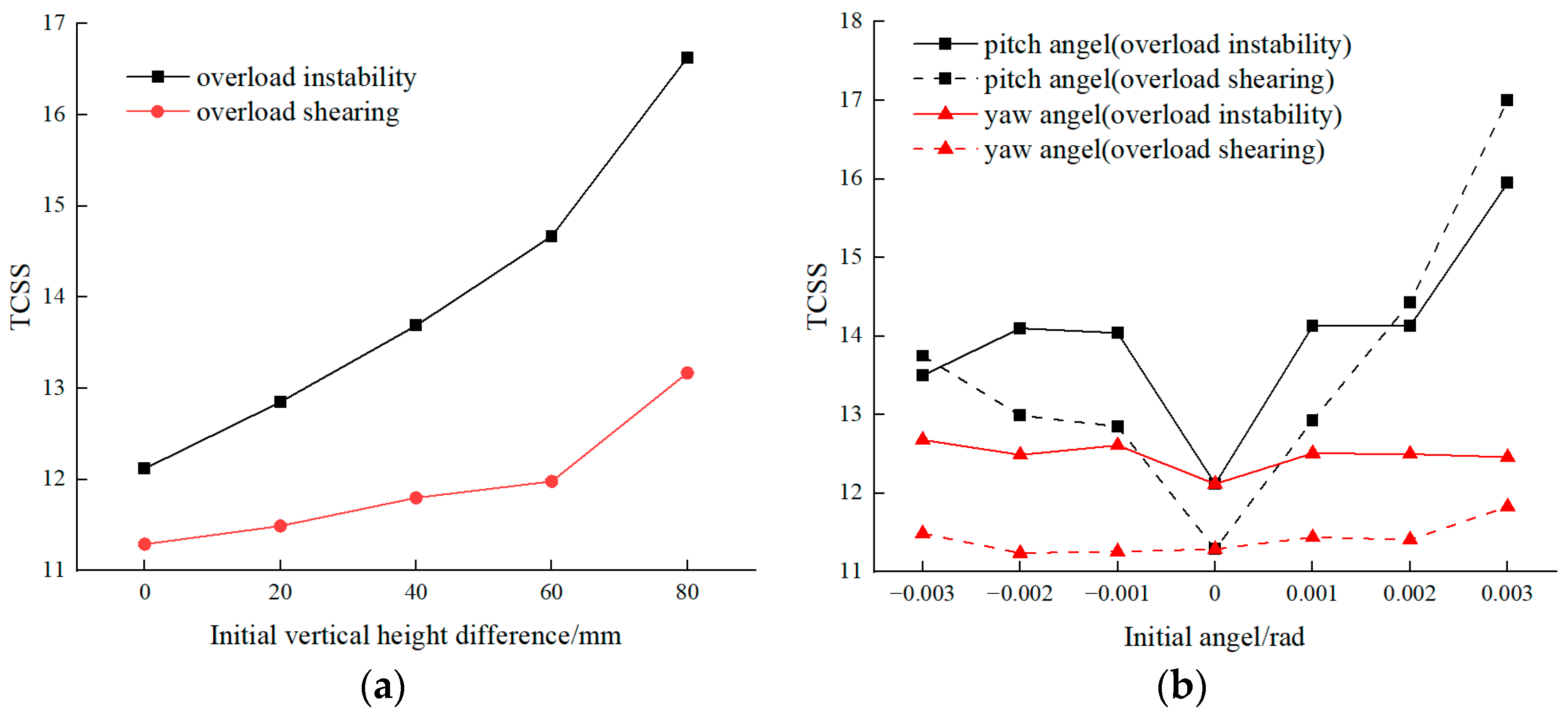
4.3. The Influence of Initial Attitude on Collisions

The influence of factors such as curved track, uneven rail conditions, and lateral oscillation may cause vertical lift, yaw, or pitch motions in the carbody before collisions. Three sets of dynamic simulation calculations were performed to investigate the influence of these factors on collisions. In the first set, the carbody of the moving train was raised by 20, 40, 60, and 80 mm. In the second set, the moving train carbody was initially set with pitch angles of −0.003, −0.002, −0.001, 0, 0.001, 0.002, and 0.003 radians. In the third set, the moving train carbody was initially set with yaw angles of −0.003, −0.002, −0.001, 0, 0.001, 0.002, and 0.003 radians.

Figure 9a illustrates the TCSS for different intermediate coupler overload states at various initial vertical heights. The greater the initial vertical height difference between the two colliding trains, the larger the TCSS after the collision. Under the same conditions, trains with coupler overload shearing have lower TCSS values than those with overload instability after the collision. Figure 9b illustrates the TCSS for different intermediate coupler overload states at various initial pitch and yaw angles. An initial pitch angle significantly increases the TCSS after the collision, while the yaw angle minimizes the TCSS. Additionally, positive pitch angles have a greater impact on increasing TCSS than negative ones. When an initial yaw angle is present, trains with coupler overload shearing have lower TCSS values than trains with overload instability after the collision.

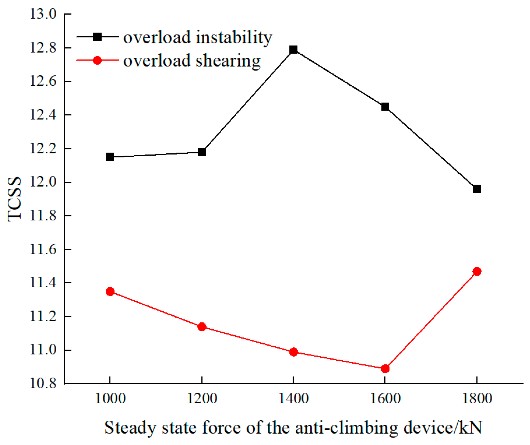
4.4. The Influence of Leading Car Energy-Absorbing Device Parameters on Collisions

During a frontal collision, the central collision interface absorbs much of the collision energy, making the parameter settings of the leading car energy-absorbing device crucial for collision response. The leading car energy-absorbing device comprises a leading coupler and an anti-climbing device. The primary energy-absorbing component of the leading coupler is the collapse tube. Six different combinations of stroke and force have been designed while maintaining an equal energy absorption capacity for the collapse tube. The specific scheme configurations and TCSS values for different schemes can be found in

Table 4. Combination schemes of the heading coupler collapse tube.

Scheme	Stroke/ mm	Force/ kN	TCSS
			Overload Instability	Overload Shearing
Scheme 1	1620	1200	12.21	11.50
Scheme 2	1500	1300	12.22	11.27
Scheme 3	1390	1400	12.33	11.35
Scheme 4	1300	1500	12.15	11.35
Scheme 5	1220	1600	12.20	11.50
Scheme 6	1150	1700	12.16	11.40

. The response after the collision varies depending on the overload state of the intermediate coupler. As the force level of the collapse tube increases, the TCSS of the train with overload instability exhibits a trend of initially increasing and then decreasing. In contrast, the TCSS of the train with overload shearing shows a trend of initially decreasing and then increasing. In overall comparison, trains with intermediate coupler overload shearing have smaller TCSS values. Therefore, selecting an appropriate combination of collapse tube force and stroke based on different overload states of the intermediate coupler can effectively enhance collision safety.

The heading anti-climbing device emerges when the heading coupler fails due to shearing. Without changing other parameters, the force levels of the heading anti-climbing device are set to 1000, 1200, 1400, 1600, and 1800 kN for simulation calculations. The variation of the TCSS of the anti-climbing device with increasing steady-state force level is shown in Figure 10. Similar to the impact of the collapse tube in the coupler on TCSS, different overload states of the intermediate coupler exhibit diverse trends. Therefore, the selection of force levels for the anti-climbing device is not necessarily “the higher, the better”. Choosing appropriate force levels based on the actual situation is necessary to achieve lower TCSS values.

5. Conclusions

To investigate the issue of high-speed frontal train collisions, this study establishes a vehicle–track coupled model with a three-dimensional vehicle model consisting of 38 degrees of freedom and a fixed three-layer vibrating track model. Additionally, several algorithms are developed, including a wheel–rail contact algorithm based on Hertz contact theory, a geometry-based car–end contact algorithm, and a nonlinear representation method for the entire process of the intermediate coupler. These components collectively constitute a collision dynamic model suitable for higher collision velocities. The main conclusions of this study are as follows:

(1)

The collision dynamic model considers the wheel–rail contact, car–end contact, and coupler overload issues in high-speed collisions. Based on mathematical models, simulation programs are developed to effectively simulate and calculate the problem of high-speed frontal train collisions;

(2)

A calculation method for car–end contact is established based on a typical compliant contact model, which can be used in the collision dynamic model. An engineering determination method for the coefficients in the calculation method is studied through finite element numerical simulations, enabling rapid calculation of the car–end contact force;

(3)

A collision dynamic simulation is conducted on a specific model of a high-speed train to investigate the impact of the initial attitude and parameters of the leading energy-absorption device on collision safety. The results indicate that an initial height difference and yaw angle will increase TCSS, making the train more dangerous after the collision;

(4)

Different overload states of the intermediate coupler lead to different effects of parameter variations in the leading energy-absorption device on TCSS. For trains with overload instability, TCSS shows a trend of initially increasing and then decreasing with the increase in force level of the energy-absorption device after the collision. On the other hand, trains with overload shearing exhibit the opposite trend. Therefore, it is necessary to select appropriate force levels for the energy-absorption device based on the actual situation.

Through the study in this paper, it is possible to rationally configure the parameters of the energy-absorption device under different collision velocities at the early stage of train design and improve the safety of the train after a frontal collision. However, to obtain more accurate calculation results, it is crucial to establish more elaborate vehicle models and develop more accurate car–end contact algorithms in future research. In addition, it is worth further research to establish a comprehensive and extensive model to predict the posture of trains after collision in different situations.

References

1. Evans, A.W. Fatal train accidents on Europe’s railways: An update to 2019. Accid. Anal. Prev. 2021, 158, 106182. [Google Scholar] [CrossRef] [PubMed]
2. Lin, C.-Y.; Rapik Saat, M.; Barkan, C.P. Quantitative causal analysis of mainline passenger train accidents in the United States. Proc. Inst. Mech. Eng. Part F J. Rail Rapid Transit 2020, 234, 869–884. [Google Scholar] [CrossRef]
3. Xu, T.; Xu, P.; Zhao, H.; Yang, C.; Peng, Y. Vehicle running attitude prediction model based on Artificial Neural Network-Parallel Connected (ANN-PL) in the single-vehicle collision. Adv. Eng. Softw. 2023, 175, 103356. [Google Scholar] [CrossRef]
4. Severson, K.J.; Parent, D.P.; Tyrell, D.C. (Eds.) Two-Car Impact Test of Crash-Energy Management Passenger Rail Cars: Analysis of Occupant Protection Measurements. In Proceedings of the ASME 2004 International Mechanical Engineering Congress and Exposition, Anaheim, CA, USA, 13 November 2004. [Google Scholar]
5. Tyrell, D.; Jacobsen, K.; Martinez, E. (Eds.) Train-to-Train Impact Test of Crash Energy Management Passenger Rail Equipment: Structural Results. In Proceedings of the ASME 2006 International Mechanical Engineering Congress and Exposition, Chicago, IL, USA, 5–10 November 2006. [Google Scholar]
6. Tyrell, D.; Severson, K.; Perlman, A.B. (Eds.) Rail Passenger Equipment Crashworthiness Testing Requirements and Implementation. In Proceedings of the ASME 2000 International Mechanical Engineering Congress and Exposition, Cambridge, MA, USA, 6 November 2000. [Google Scholar]
7. Sutton, A. The development of rail vehicle crashworthiness. Proc. Inst. Mech. Eng. Part F J. Rail Rapid Transit 2002, 216, 97–108. [Google Scholar] [CrossRef]
8. Yao, S.; Yan, K.; Lu, S.; Xu, P. Energy-absorption optimisation of locomotives and scaled equivalent model validation. Int. J. Crashworth. 2017, 22, 1–12. [Google Scholar] [CrossRef]
9. Yu, Y.; Gao, G.; Guan, W.; Liu, R. Scale similitude rules with acceleration consistency for trains collision. Proc. Inst. Mech. Eng. Part F J. Rail Rapid Transit 2018, 232, 2466–2480. [Google Scholar] [CrossRef]
10. Li, J.; Gao, G.; Yu, Y.; Li, J. Similitude scaled method for three-dimensional train collision. Proc. Inst. Mech. Eng. Part F J. Rail Rapid Transit 2022, 237, 1–12. [Google Scholar] [CrossRef]
11. Lu, S.; Wang, P.; Ni, W.; Yan, K.; Chen, Z. A mechanical equivalence similitude method for dynamic responses of high-speed train middle vehicles in a collision. Proc. Inst. Mech. Eng. Part F J. Rail Rapid Transit 2022, 237, 1–12. [Google Scholar] [CrossRef]
12. Meran, A.P.; Baykasoglu, C.; Mugan, A.; Toprak, T. Development of a design for a crash energy management system for use in a railway passenger car. Proc. Inst. Mech. Eng. Part F J. Rail Rapid Transit 2016, 230, 206–219. [Google Scholar] [CrossRef]
13. Yao, S.; Zhu, H.; Yan, K.; Liu, M.; Xu, P. The derailment behaviour and mechanism of a subway train under frontal oblique collisions. Int. J. Crashworth. 2021, 26, 133–146. [Google Scholar] [CrossRef]
14. Baykasoglu, C.; Mugan, A.; Sunbuloglu, E.; Bozdag, S.E.; Aruk, F.; Toprak, T. Rollover crashworthiness analysis of a railroad passenger car. Int. J. Crashworth. 2013, 18, 492–501. [Google Scholar] [CrossRef]
15. Bae, H.-U.; Yun, K.-M.; Lim, N.-H. Containment capacity and estimation of crashworthiness of derailment containment walls against high-speed trains. Proc. Inst. Mech. Eng. Part F J. Rail Rapid Transit 2018, 232, 680–696. [Google Scholar] [CrossRef]
16. Wei, L.; Zhang, L.; Tong, X.; Cui, K. Crashworthiness study of a subway vehicle collision accident based on finite-element methods. Int. J. Crashworth. 2021, 26, 159–170. [Google Scholar] [CrossRef]
17. Song, Z.; Ming, S.; Li, T.; Du, K.; Zhou, C.; Wang, B. Improving the energy absorption capacity of square CFRP tubes with cutout by introducing chamfer. Int. J. Mech. Sci. 2021, 189, 105994. [Google Scholar] [CrossRef]
18. Yang, H.; Lei, H.; Lu, G. Crashworthiness of circular fiber reinforced plastic tubes filled with composite skeletons/aluminum foam under drop-weight impact loading. Thin-Walled Struct. 2020, 160, 107380. [Google Scholar] [CrossRef]
19. Baroutaji, A.; Arjunan, A.; Stanford, M.; Robinson, J.; Olabi, A.G. Deformation and energy absorption of additively manufactured functionally graded thickness thin-walled circular tubes under lateral crushing. Eng. Struct. 2021, 226, 111324. [Google Scholar] [CrossRef]
20. Tang, Z.; Liu, F.J.; Guo, S.H.; Chang, J.; Zhang, J.J. Evaluation of coupled finite element/meshfree method for a robust full-scale crashworthiness simulation of railway vehicles. Adv. Mech. Eng. 2016, 8, 2071833383. [Google Scholar] [CrossRef]
21. Xie, S.; Yang, W.; Ping, X. Simulation Analysis of a Multiple-Vehicle, High-Speed Train Collision Using a Simplified Model. Shock Vib. 2018, 2018, 9504141. [Google Scholar] [CrossRef]
22. Yuan, C.B. Study on Longitudinal Impact Modeling and Energy Management Based on Train Collision Dynamics. Master’s Thesis, Southwest Jiaotong University, Chengdu, China, 2018. [Google Scholar]
23. Dias, J.; Pereira, M.S. Analysis and design for train crashworthiness using multibody models. Veh. Syst. Dyn. 2004, 40, 107–120. [Google Scholar]
24. Ling, L.; Guan, Q.; Dhanasekar, M.; Thambiratnam, D.P. Dynamic simulation of train–truck collision at level crossings. Veh. Syst. Dyn. 2017, 55, 1–22. [Google Scholar] [CrossRef]
25. Hou, L.; Peng, Y.; Sun, D. Dynamic analysis of railway vehicle derailment mechanism in train-to-train collision accidents. Proc. Inst. Mech. Eng. Part F J. Rail Rapid Transit 2021, 235, 1022–1034. [Google Scholar] [CrossRef]
26. Zhou, H.; Zhan, J.; Zhang, C. Simulation of the city tram collision at the level crossing. J. Mech. Eng. 2018, 54, 35–40. [Google Scholar] [CrossRef]
27. Zhou, H.; Wang, W.; Hecht, M. Three-dimensional derailment analysis of a crashed city tram. Veh. Syst. Dyn. 2013, 51, 1200–1215. [Google Scholar] [CrossRef]
28. Yang, C. Research on Key Issues of Train Collision Dynamics. Ph.D. Thesis, Southwest Jiaotong University, Chengdu, China, 2016. [Google Scholar]
29. Wang, K.W. Calculation of the wheel contact trajectory and wheel-rail contact geometric parameters. J. Southwest Jiaotong Univ. 1984, 1, 89–99. [Google Scholar]
30. Luo, L.; Nahon, M. Development and Validation of Geometry-Based Compliant Contact Models. J. Comput. Nonlinear Dyn. 2010, 6, 011004. [Google Scholar] [CrossRef]
31. Luo, L. Development and validation of a geometry-based contact force model. Ph.D. Thesis, McGill University, Montreal, QC, Canada, 2010. [Google Scholar]
32. Zhang, J.; Zhu, T.; Yang, B.; Wang, X.; Xiao, S.; Yang, G.; Liu, Y. Collision characteristics of the intermediate coupler of a rail vehicle. Veh. Syst. Dyn. 2022, 1–22. [Google Scholar] [CrossRef]
Figure 1. Three-dimensional train collision dynamic model.
Applsci 13 10805 g001
Figure 2. Sketch of the simplified section of car ends. (a) Simplified section of the cab end; (b) simplified section of the intermediate car end.
Applsci 13 10805 g002
Figure 3. Finite element model and dimensions. (a) Sketch of the impact model; (b) sketch of the validation model.
Applsci 13 10805 g003
Figure 4. Load–deformation relationship under impact loading.
Applsci 13 10805 g004
Figure 5. Mathematical model of the coupler. (a) The composite curve method; (b) Representation of the compression state throughout the entire collision process of the intermediate coupler.
Applsci 13 10805 g005
Figure 6. Flowchart of the dynamic calculation program.
Applsci 13 10805 g006
Figure 7. Collision scenario.
Applsci 13 10805 g007
Figure 8. Instability characteristic curve of the intermediate coupler.
Applsci 13 10805 g008
Figure 9. The influence of initial attitude on collisions. (a) Initial vertical height differences; (b) initial angles.
Applsci 13 10805 g009
Figure 10. The influence of anti-climbing device on collisions.
Applsci 13 10805 g010