Abstract
Knee orthosis plays a vital role in enhancing the wellbeing and quality of life of individuals suffering from knee arthritis. This study explores a machine-learning-based methodology for predicting a user’s gait subphase using inertial measurement units (IMUs) for a semiactive orthosis. A musculoskeletal simulation is employed with the help of existing experimental motion-capture data to obtain essential metrics related to the gait cycle, which are then normalized and scaled. A meticulous data capture methodology using foot switches is used for precise synchronization with IMU data, resulting in comprehensive labeled subphase datasets. The integration of simulation results and labeled datasets provides activation data for effective knee flexion damping following which multiple supervised machine learning algorithms are trained and evaluated for performances. The time series forest classifier emerged as the most suitable algorithm, with an accuracy of 86 percent, against randomized convolutional kernel transform, K-neighbor time series classifier, and long short-term memory–fully convolutional network, with accuracies of 68, 76, and 78, respectively, showcasing exceptional performance scores, thereby rendering it an optimal choice for identifying gait subphases and achieving the desired level of damping for magnetorheological brake-mounted knee orthosis based on simulated results.
1. Introduction
Osteoarthritis (OA) is a common form of arthritis categorized as primary or secondary, typically involving pain and restricted joint movement. Its clinical presentation can vary from asymptomatic to debilitating and persistent [1]. Gait encompasses the coordinated movement of limbs during activities like walking and running. It involves the integration of multiple body systems, including musculoskeletal, nervous, and cardiovascular. The study of gait is valuable in fields like biomechanics, physical therapy, and rehabilitation, enabling insights into movement mechanisms and the detection of abnormalities or impairments impacting mobility [2]. Patients experiencing long-term osteoarthritis exhibit notable alterations in their usual gait pattern, including heightened external rotation, decreased articulation speed, and abnormal stance phase flexion that inadequately supports proper weight bearing [3]. A knee orthosis (KO) coupled with some damping mechanism is a relatively new concept, and the use of a magnetorheological (MR) brake is a promising application [4]. One of the major challenges is to devise a mechanism to significantly increase the mechanical advantage while keeping the weight of the device to a minimum by the use of a compact, lightweight gear reduction system. Significant advances have been made in the field of material sciences, and composites even pose mechanical strength for the knee joint [5]. The knee moment is the force exerted on the knee joint during the gait cycle. Deviations from normal knee moment patterns can indicate potential mobility issues and biomechanical abnormalities. Increased knee moment can contribute to knee injuries and affect mobility and quality of life. Conversely, decreased knee moment may lead to instability and reduced force transmission, impacting gait patterns and mobility. Assessing knee moment and its relationship with gait provides valuable insights for guiding treatment and rehabilitation strategies to address specific gait abnormalities and improve overall mobility [6].
Machine learning, a subset of artificial intelligence, is focused on enabling computer systems to improve their performance on specific tasks without being explicitly programmed. This field involves the utilization of algorithms that learn from data through mathematical and statistical methodologies, allowing them to recognize patterns and relationships. By leveraging these acquired patterns and relationships, machine learning algorithms can make predictions, uncover hidden insights, and accomplish various tasks [7]. Gait subphase detection entails the utilization of machine learning techniques to identify and categorize various subphases within the gait cycle. These subphases are specific windows of time where the detection and activation of the MR brake occur to control knee flexion and assess knee stress based on the knee moment parameter. By analyzing gait data using machine learning algorithms, it becomes possible to automatically recognize and distinguish various subphases, such as heel strike, toe-off, swing phase, and stance phase, among others. This approach provides a more precise and comprehensive understanding of gait patterns, offering potential advancements in areas like clinical assessment, rehabilitation, and biomechanical research involving human movement [8]. C. Prakash et al. described a unique method for identifying gait phases by utilizing an optical approach with passive markers. It uses fuzzy logic to automatically recognize different subphases of gait, resulting in a precise and reliable measurement useful for analyzing gait abnormalities in patients and for the use in the development of control strategies for active lower-extremity prosthetics and orthotics [9]. Taborri et al. proposed a distributed classifier for gait phase detection in an active knee orthosis for pediatric subjects with neurological diseases. The classifier utilizes a hierarchical weighted decision framework applied to scalar hidden Markov models trained on kinematic data from the shank and thigh. Results show that the classifier based on angular velocities achieves higher sensitivity and specificity. Utilizing additional linear acceleration data does not improve performance, suggesting a need for a gait phase detection algorithm based on gyroscopes placed on the shank and thigh for the orthosis implementation [10].
The objective of this study is to develop a methodology for identifying gait phases and determining the activation level of a magnetorheological brake-mounted knee orthosis based on simulated gait knee moment. The application of a time forest tree classifier algorithm proves effective in accurately identifying gait phases, while the knee moment is obtained through an OpenSim simulation of the gait. Foot switches are utilized to collect data for labeling and to determine the individual percentage gait share. Through this approach, the study aims to provide insights into accurately identifying gait phases and quantifying the activation level of the knee orthosis based on knee moment during simulated gait.
2. Musculoskeletal Simulation
OpenSim 4.4 (SimTK: National Institutes of Health (NIH), Bethesda, MD, USA) is an open-source software developed at Stanford University for musculoskeletal simulation and biomechanical modeling. It enables the creation of detailed models to study human movement and assess joint movements, muscle forces, and energy consumption during activities. It is widely used in biomedical engineering and biomechanics, offering valuable insights into the effects of injuries, diseases, surgical interventions, and the design of prosthetics or therapeutic interventions [11]. The objective of the simulation is to perform inverse kinematics to obtain joint angles. With the results, inverse dynamics is performed to obtain joint reaction forces and moments. The simulation utilizes existing motion capture data for inverse kinematics, which is then combined with ground reaction force data sourced online and associated with a generic model. The objective is to obtain a normalized and scaled knee moment for one gait cycle, without requiring any experimental data input other than scaling the model to match the subject’s specific anthropometry (physical dimensions), and the inertial parameters of the model are given in Table 1 [12].

Table 1.
Model inertial parameters [12].
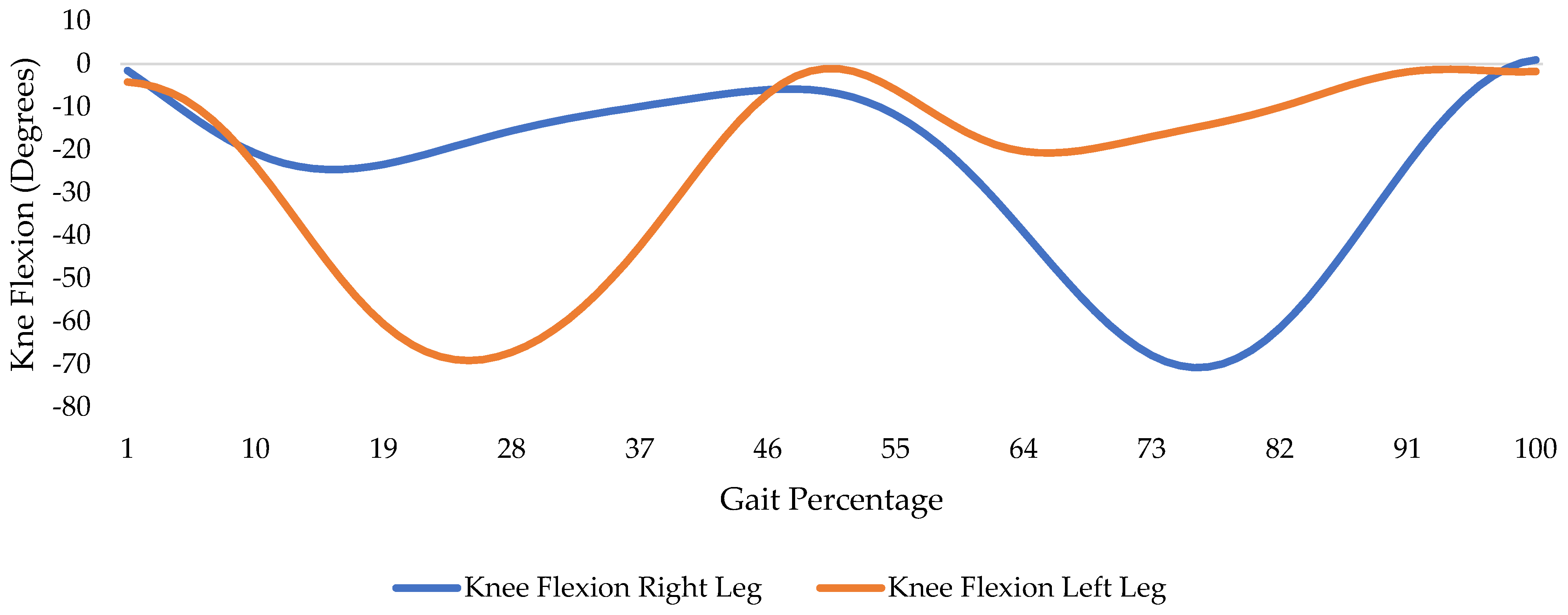
The simulation involves performing inverse kinematics on a scaled model of the subject’s musculoskeletal system. The output knee flexion is shown in Figure 1; it was corrected for gait phase alignment and is scaled for one complete gait cycle.
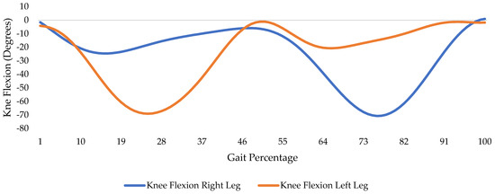
Figure 1.
Simulated knee flexion of both legs.
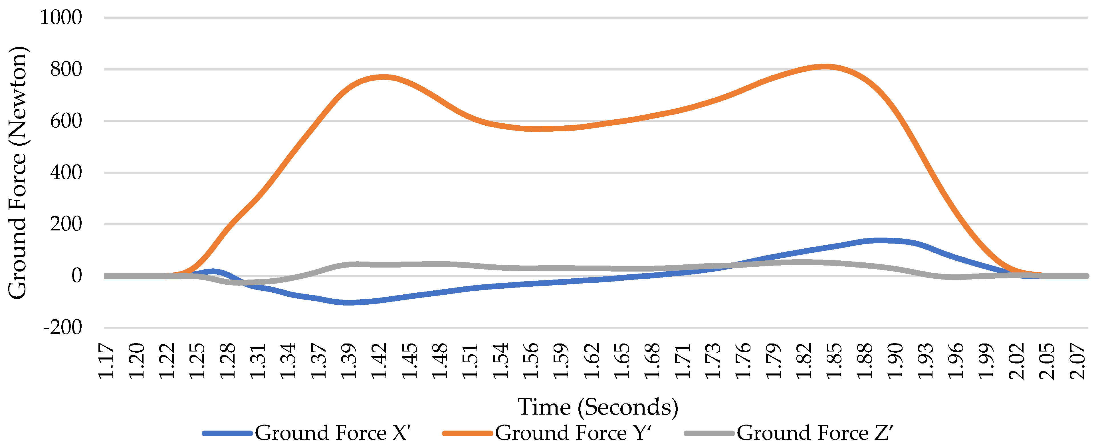
The process of inverse dynamic simulation encompasses 76 frames, which are captured using motion capture techniques. In this process, force data associated with the leg-mounted force plates, as shown in Figure 2, are obtained from the repository. These force plates provide measurements of forces in the X′, Y′, and Z′ directions, corresponding to the frontal, transverse, and sagittal planes, respectively [13]. These techniques capture the subject’s movements by strategically placing markers on their body to trace a complete gait cycle.
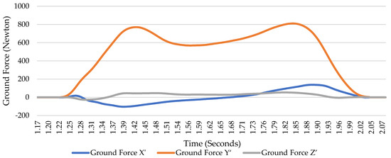
Figure 2.
Ground forces along different axes.
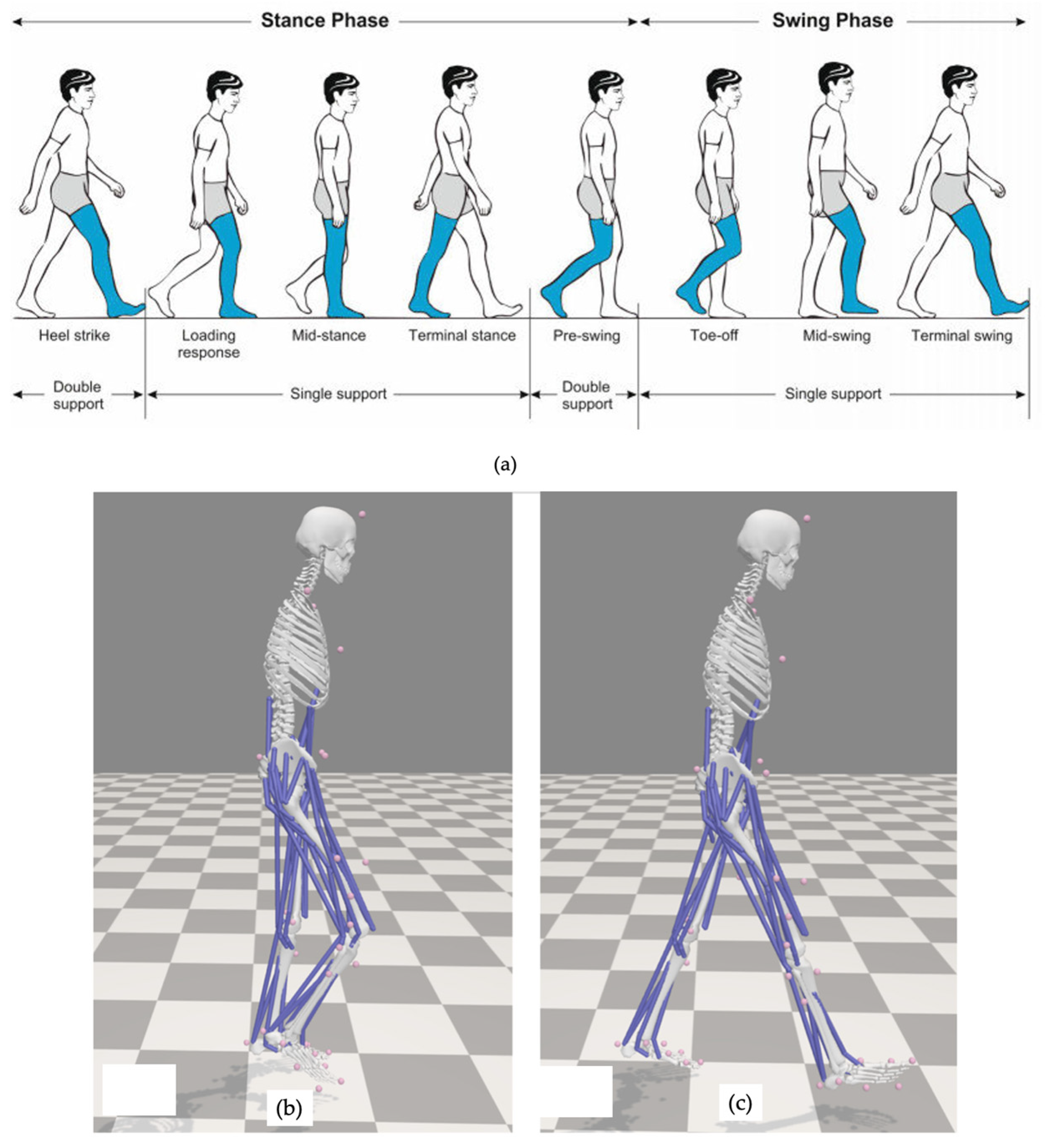
To establish alignment between the knee flexion pattern simulated during the gait and the designated zero state (representing heel strike Figure 3c), a phase shift is implemented. The alignment process is shown in Figure 3 for synchronization between the simulated knee flexion and the defined starting state. The objective of inverse dynamics is the determination of the forces and moments responsible for a particular motion, thereby elucidating the muscular contributions underlying said motion. The attainment of these forces and moments involves a methodical iterative solution of the system’s equations of motion. These equations of motion encompass a comprehensive consideration of the kinematic characteristics and mass attributes inherent in a model of the musculoskeletal system.
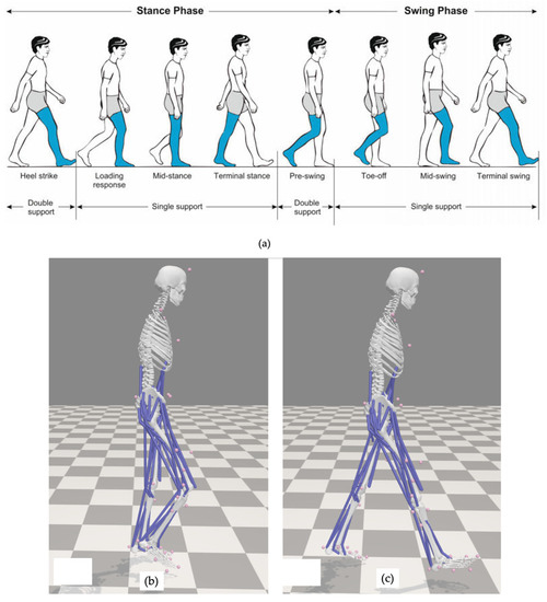
Figure 3.
(a) Gait phases; (b) nominal gait starting phase from simulation; (c) corrected gait starting phase.
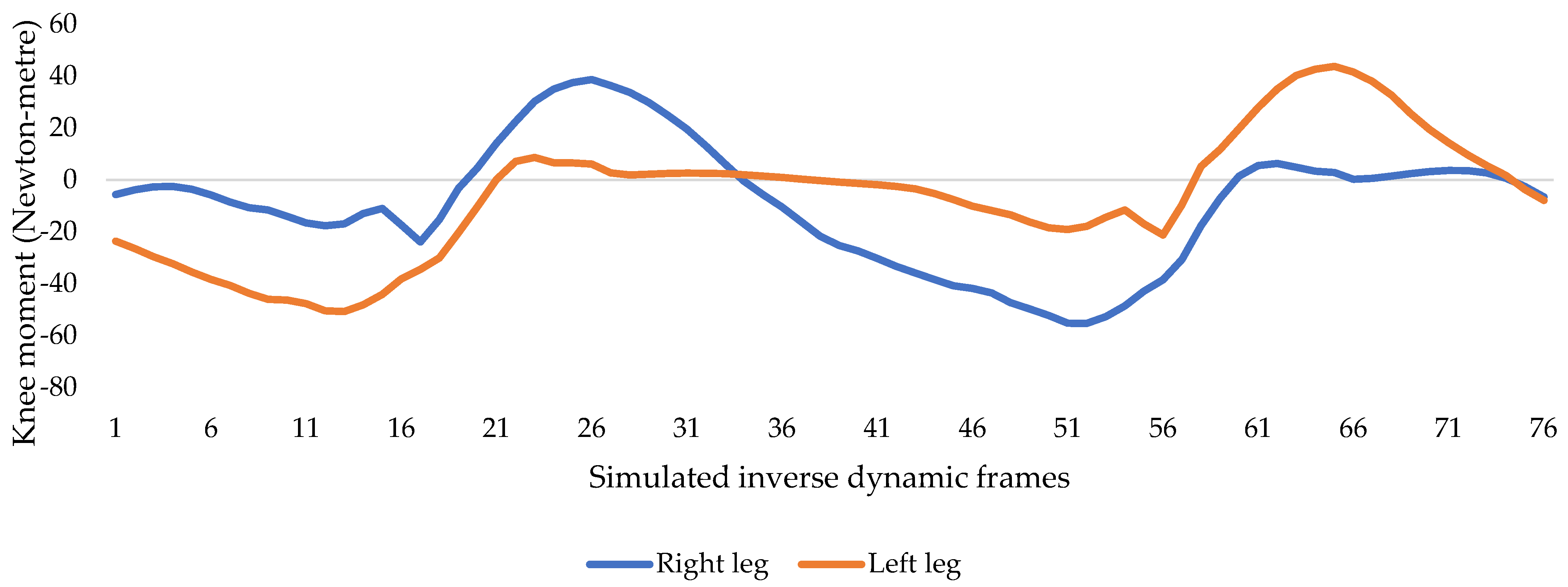
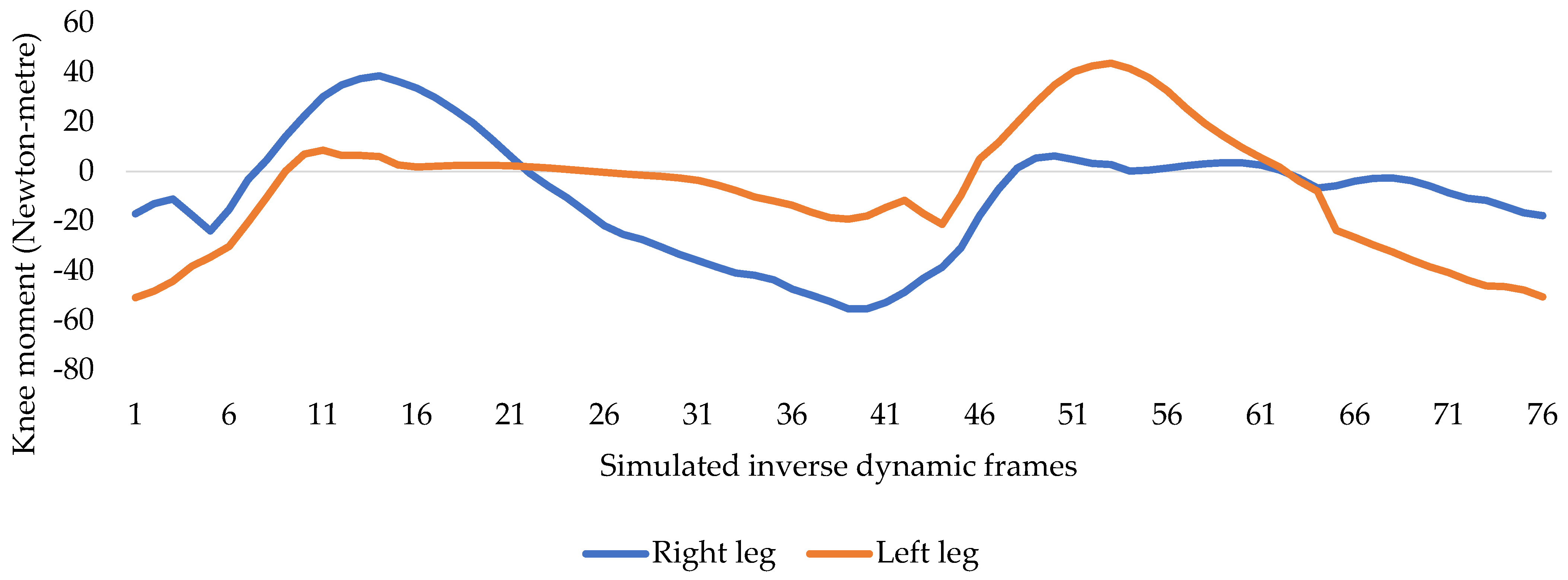
Utilizing the joint angles derived from the principles of inverse kinematics and informed by experimental data pertaining to ground reaction forces, the resultant reactive forces and moments acting upon each joint can be effectively calculated. Notably, this calculation adheres rigorously to the imperatives of dynamic equilibrium and the constraints imposed by the system’s boundaries [14]. The output in Figure 4 is the nominal output from the simulation performed on the scaled musculoskeletal model, which is not corrected for the phase shift of gait. A simple slicing of the data points and placing them in the end position results in a phase-corrected gait cycle, as shown in Figure 5.
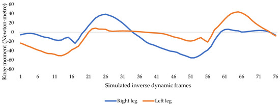
Figure 4.
Simulated knee output moments.
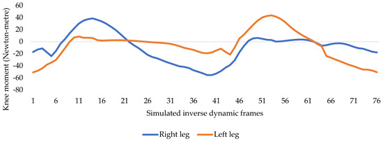
Figure 5.
Phase-shifted knee moments.
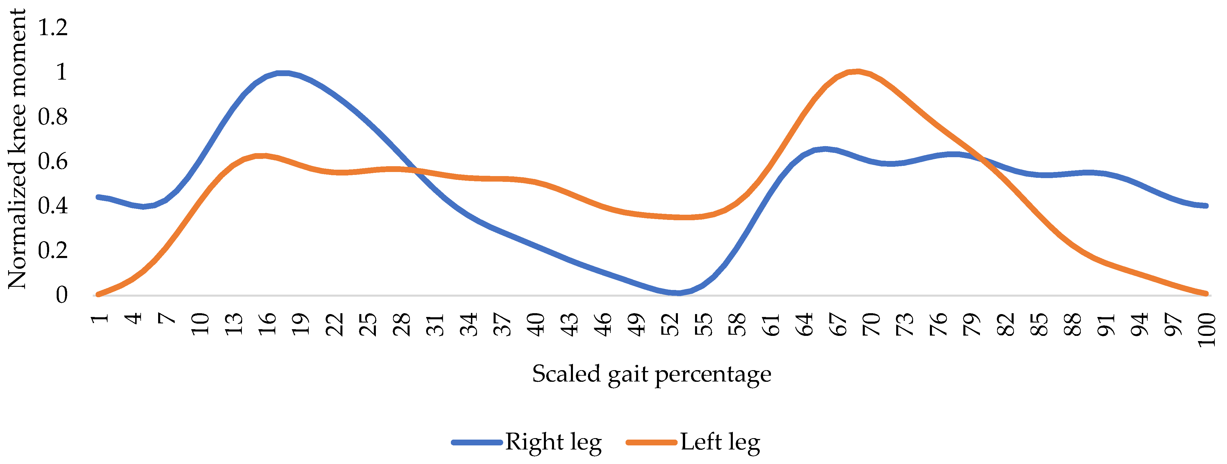
Further, the gait cycle is normalized for the moment and the output is shown in Figure 6. The inverse dynamics is performed in 76 different frames; therefore, the output has 76 data points. To scale them, the MATLAB curve fitting toolbox is used and an optimum balance between preserving the profile and accuracy is reached by the use of a sum of the sine curve, as shown by Equation (1), and selecting subsequent coefficients for both the curves with the final moment profile in Figure 6.
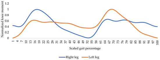
Figure 6.
Normalized, phase-shifted, and scaled knee moments.
In this application, prioritizing the moment parameter associated with specific gait subphases over knee flexion is more suitable. Figure 6 depicts knee moments throughout the gait cycle and offers valuable insights for enhancing patient ambulation. This entails engaging the orthosis brake to align flexion damping with the moment profile, offering supportive assistance. The choice to eschew knee flexion as a braking parameter arises from instances where knee flexion lacks consistent strain correlation. Additionally, cases involving weight transfer to the contralateral knee may present lower flexion but heightened strain, further justifying the moment parameter’s preference.
3. Gait Phase Segregation and Percentage Share
IMU data acquisition involves the use of footswitch data acquired simultaneously with two different IMUs’ angular displacement and acceleration of the right leg for labeling the gait phases. A frequency distribution analysis is performed on the labeled data and an averaged gait percentage share is obtained. This helps to identify the share of each gait subphase in one gait cycle and its relative importance, and is combined with the simulated knee moment. This acts as a marker for the time period when the knee joint is under strain. The IMU Adafruit BNO085 is equipped with a 9-DoF (degrees of freedom) sensor fusion algorithm, incorporating data from the accelerometer, gyroscope, and magnetometer. Combining the data from multiple sensors provides orientation estimates that are more accurate and reliable, effectively reducing the likelihood of a gimbal lock. Furthermore, it has autocalibration support, allowing continuous updating of calibration parameters to compensate for factors such as temperature variations or sensor aging. The sensor is accompanied by a proprietary motion engine that utilizes the Mahony and Madgwick sensor fusion algorithms. These algorithms estimate orientation by considering sensor biases, noise, and other characteristics, resulting in enhanced accuracy and stability. A normalized gait cycle is obtained with a percentage share of each phase. Together, these two sets of information are used to obtain the gait phase activation cycle with the corresponding magnitude. Roll, pitch, and yaw associated with IMUs with units in degrees are collected from the sensor’s onboard motion engine along with acceleration along the three axes to make the model more generalized when analyzing actual gait, which has variations in data output from two IMUs mounted on the thigh and shin of the right leg (only right leg is considered for data collection and testing) shown in Table 2.
Table 2.
Headers for data collection.
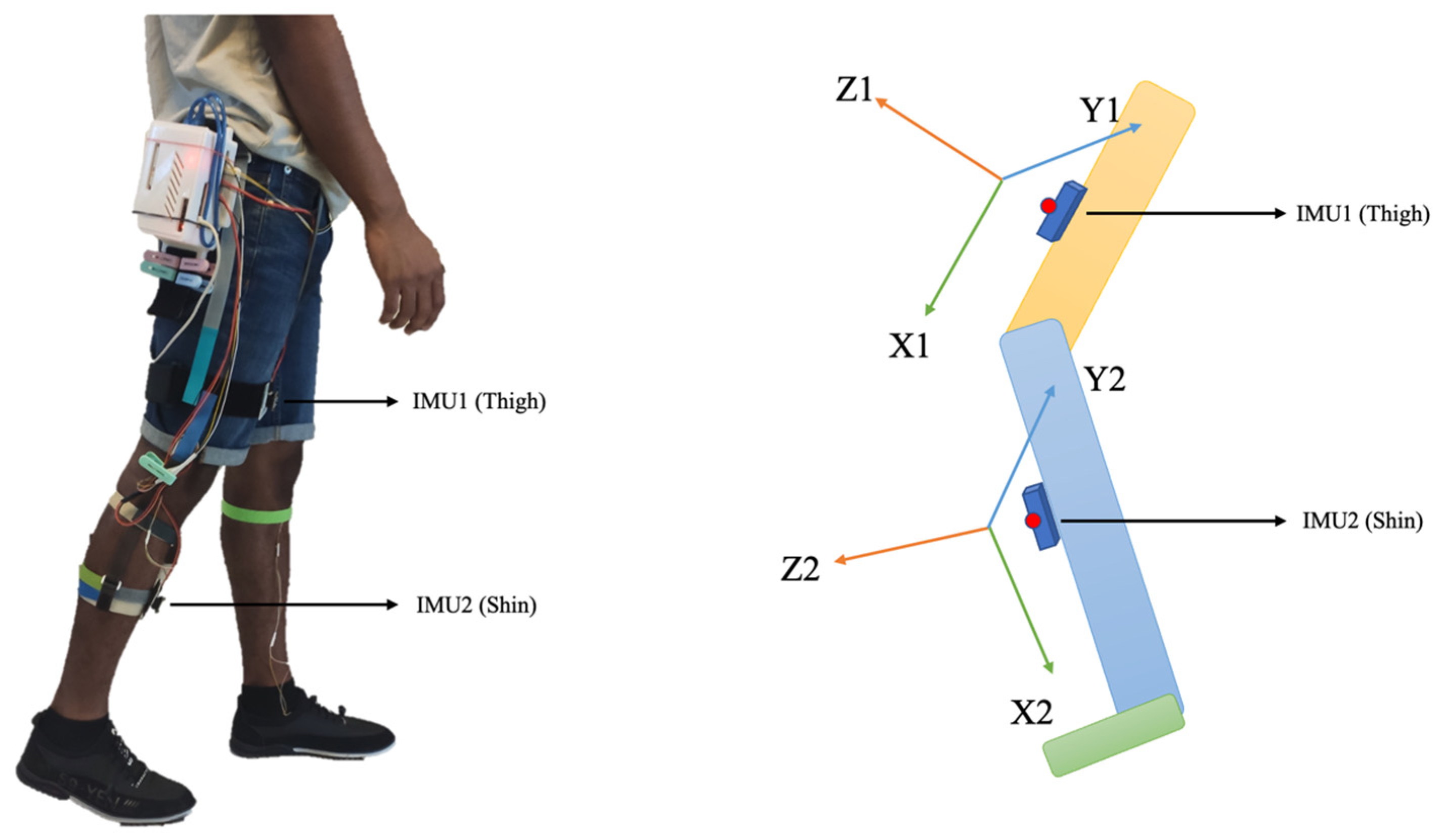
The knee flexion is captured with a pair of IMUs mounted on the thigh and shin, shown in Figure 7, with X1 and X2 denoting angular displacement along the transverse plane, Y1 and Y2 denoting angular displacement along the sagittal plane, and Z1 and Z2 denoting angular displacement along the frontal plane.
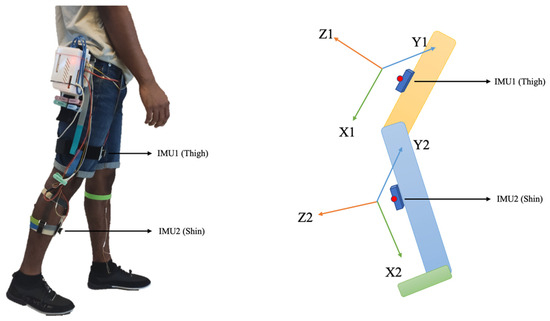
Figure 7.
IMU placement and axial description.
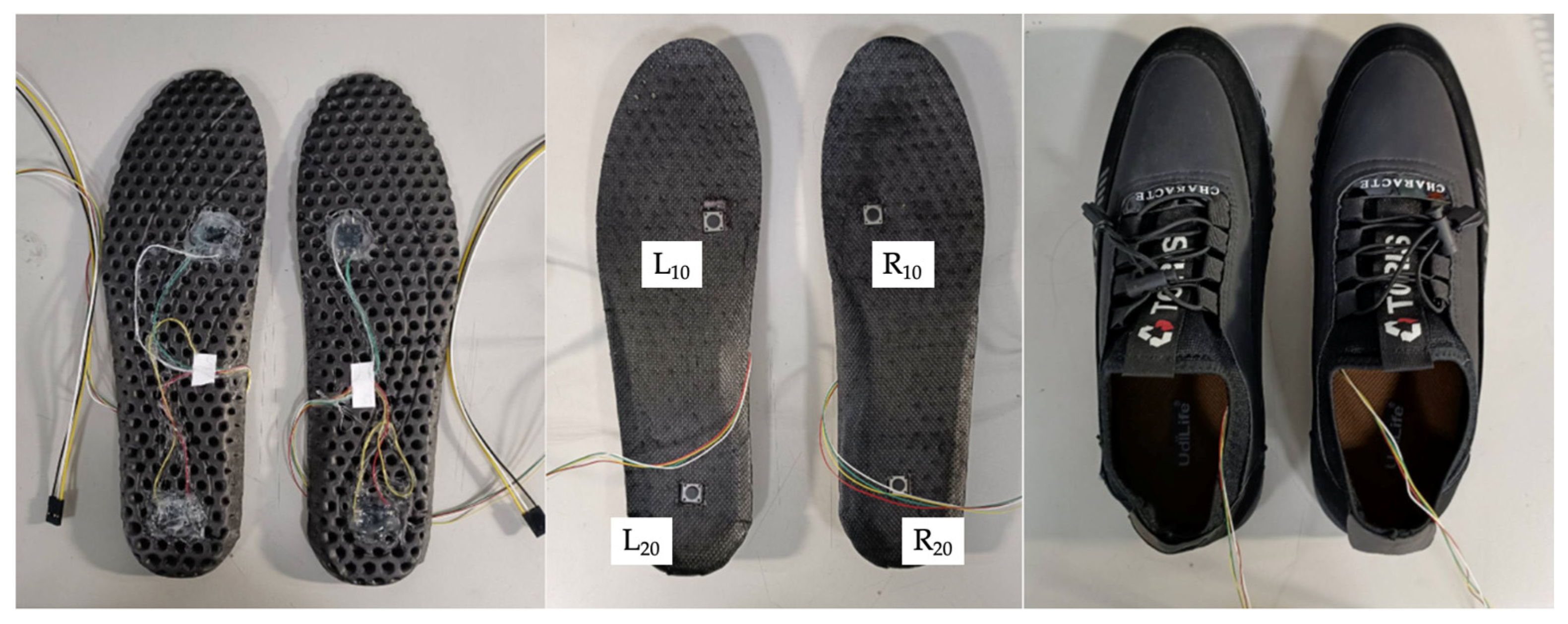
The use of four-foot switches, two for each leg mounted on the sole under the heel and ball, is shown in Figure 8, toggling between active and inactive states, resulting in permutations of 24 binary states. In a normal gait, seven distinct combinations are identified, excluding the standing-still condition where full feet support is present. Some momentary states are excluded, which arise during the transition from one phase to another, and the remaining impossible states, which are not possible, are identified as shown in Table 3, where the foot switches mounted on the left leg are labeled as L10 and L20 for the ball and heel mounted switches, whereas R10 and R20 are the right leg ball and heel mounted switches. The resolution of gait when segregated with foot switches causes some of the gait to merge in a single state, as depicted in states 2, 4, and 13, whereas certain gait phases are skewed and are identified by demarking them as starting and ending states, as depicted in states 5 and 9. The dataset description is given in Table 4. The gait is divided into seven different phases, which is shown in Figure 9.
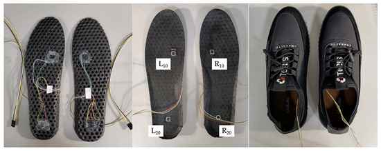
Figure 8.
Foot switch placement.
Table 3.
Ground truth table for foot switches and corresponding gait.
Table 4.
Dataset description.
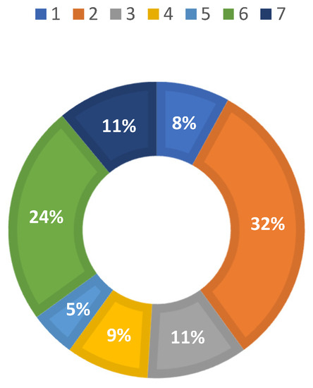
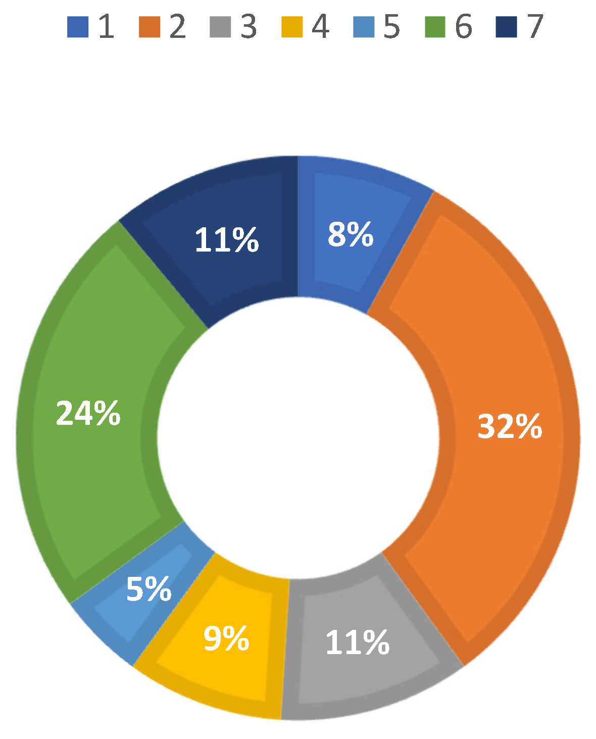
Figure 9.
Percentage share of gait phases from class 1 to 7.
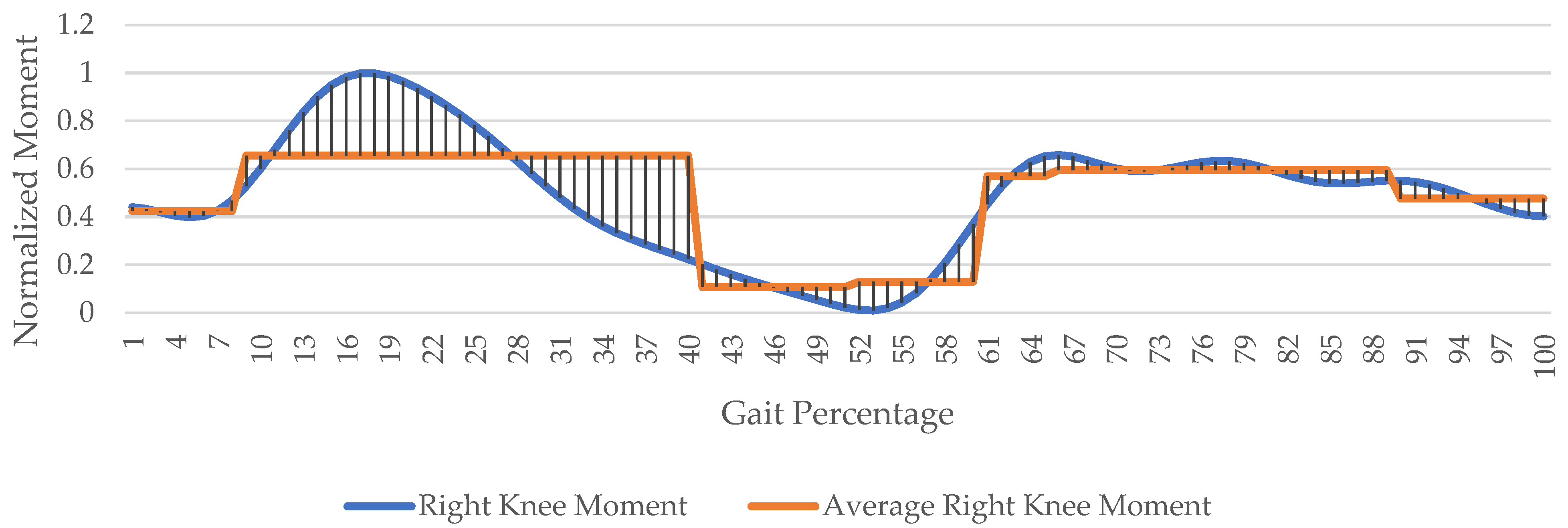
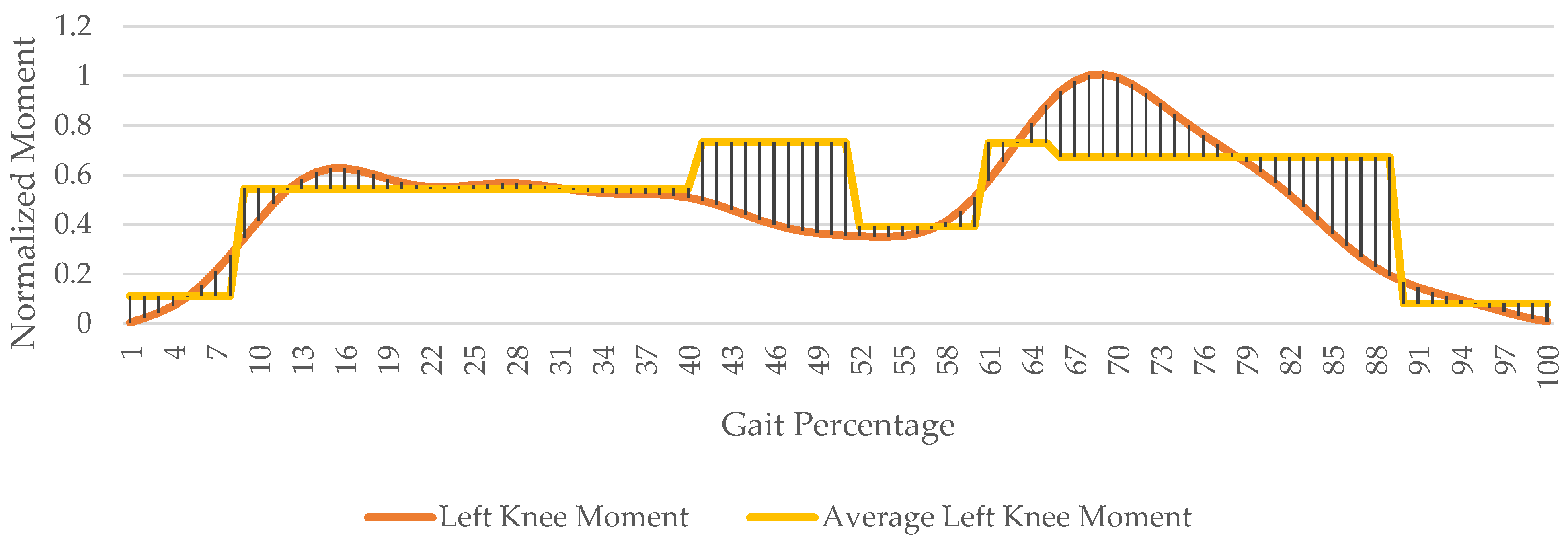
The final objective of identifying the gait phase and finding the corresponding activation level for knee damping is achieved by averaging the moment associated with each gait subphase, and a lookup table is generated, as shown in Table 5, for referenced damping. Figure 10 and Figure 11 represent the moment associated with both knees.
Table 5.
Mean and median activation for gait phases.
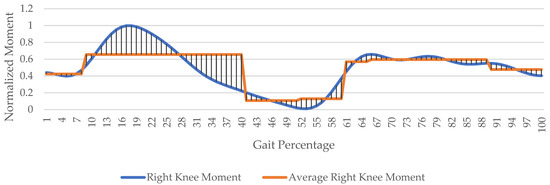
Figure 10.
Mean right knee moment associated with gait phases.
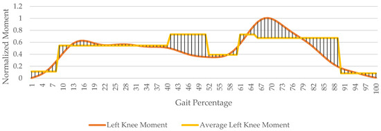
Figure 11.
Mean left knee moment associated with gait phases.
The mean time for one gait cycle ranges from 0.98 to 1.07 s [15]. The pace variation occurs for each stride. An algorithm that can predict the next gait subphase by classifying the present subphase and exploiting the Markov cycle nature of the controller gait is ideal for knee flexion damping where the next gait subphase can be known if the present subphase is identified.
Table 5 shows the mean and median brake activation corresponding to each gait phase. This is independent of the method used for damping the knee flexion. For this application, the damping is achieved by the MR brake-mounted knee orthosis; any other system devised for arresting the flexion of the knee can leverage the same data.
4. Machine Learning Algorithm for Gait Phase Identification: Training, Evaluation, and Results
For this application, four different machine learning algorithms are tested with the system specifications given in Table 6. The time series forest classifier offers interpretability through its decision-tree-based approach. ROCKET provides computational efficiency by leveraging optimized matrix operations and random convolutional kernels. LSTM–FCN combines LSTM and fully convolutional networks to capture long-term dependencies in time series. K-nearest neighbors is valued for its simplicity, flexibility, lack of a training phase, resilience to noise, and adaptability to various time series classification tasks. Evaluating and comparing these classifiers on a case-by-case basis is important, considering dataset characteristics and problem specifics, to determine the most suitable choice for a given time series classification scenario [16,17].
Table 6.
System and GPU specifications.
4.1. Time Series Forest Classifier (TSFC)
Kane et al. [18] showcased the comparative advantage and enhanced predictability of random forest for the prediction of H5N1 influenza over other state-of-the-art machine learning algorithms. An enhanced version of this algorithm, coined the hybrid random forest, was used to classify the home appliances in the household by their profile of harmonics in the current draw, which resulted in better results when time series data were fed in as parameters, wherein it performed better than other time series algorithms [19]. For the time series forest classifier (TSFC), the availability of labeled data for subphases of gait assists in the model’s supervised learning, and the random forest’s inherent ability to act as a classifier and a predictor makes it a viable choice [20]. Deng et al. [21] modified the intervals of data augmentation with a replacement that makes it a bare form of an HIVE-COTE algorithm.
The hyperparameter for the time series forest classification is based on the data type, computational resources available, and output efficiency, as shown below.
4.1.1. Number of Features
The dataset created has 12 different features that correspond to absolute orientation in degrees and acceleration associated with two IMUs. The acceleration data are requisite for stable prediction, and the absolute orientation is to counter the long-term deviations incurred as it uses the output from the onboard fusion engine in the Adafruit BNO085 chipset.
4.1.2. Number of Estimators
It defines the number of decision trees comprising the forest. For this application, 195 estimators were used to balance computational cost and acceptable results through random search.
4.1.3. Maximum Depth
The value for the maximum depth was chosen to be 10. This provides optimal performance in this application. Higher depth helps to capture the more intricate relationship of orientation data but increases the risk of overfitting. Given the variation in data, a tradeoff is achieved by avoiding the overfitting of the model.
The performance of the time series forest classifier (Figure 12) is evaluated with 1000 support variables associated with the right leg. Figure 13 shows the corresponding confusion matrix of the true and predicted classes.

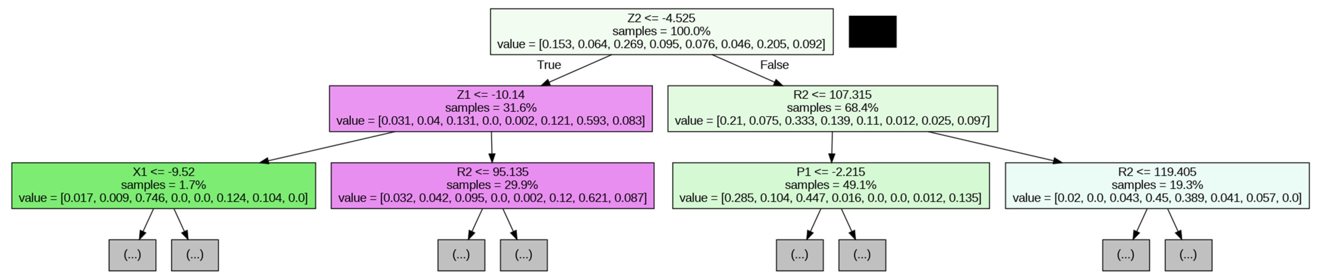
Figure 12.
Time series forest classifier architecture.
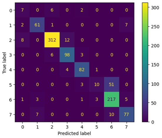
Figure 13.
Confusion matrix for time series forest classifier.
The overall accuracy of the model is 0.86 for support of 1000 occurrences in the class. The weighted average precision is 0.86. Recall is 0.86 and F1-score is 0.86, as shown in Table 7. The recall and F1-score of class 5 are very poor, which can be attributed to the minuscule number of data points associated with its 5% gait percentage share, as shown in Figure 9. Class 0 corresponds to all the activities that are irrelevant during dataset creation with no activation required.
Table 7.
Evaluation metrics for time series forest classifier.
In Figure 14, the importance of each feature is represented by corresponding to the effect it has in the decision tree during the selection of decision boundaries and classification. Here, the R2, which is associated with the “roll” of IMU mounted on the shin, affects the decision making twice as much in comparison to the roll of IMU mounted on the thigh. The “yaw” values are marginally insignificant for any decision making and can be corroborated with physical play of the leg where gait causes insignificant locomotion in the frontal plane.
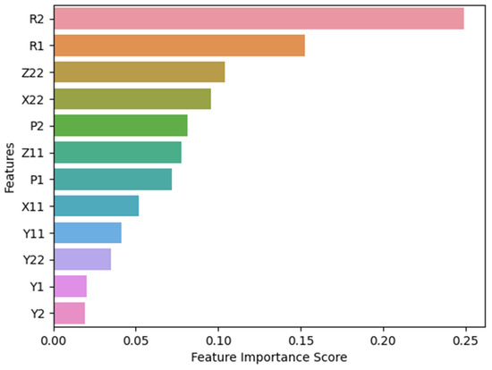
Figure 14.
Visualization of important features.
The correlation matrix in Figure 15 provides valuable insights into the relationships between all the variables within the dataset. The correlation coefficient for the model output ranges from −1 to +1 and quantifies the degree of correlation, where values close to −1 indicate a strong negative correlation, values close to +1 indicate a strong positive correlation, and values near 0 imply no correlation. Strong positive correlations among R1 and R2 depicting the roll of IMUs 1 and 2 suggest that as one variable increases, the other tends to increase as well, which is physically evident as gait involves flexion of the knee in conjunction with two IMUs. A similar trend is observed for the pitch and yaw associated with both IMUs. Also, there is a positive correlation, 0.4, of R1 (roll of IMU1) with Z22 (acceleration along Z direction for IMU2), indicating an accelerated movement of the shin (IMU2) when the thigh (IMU1) has increased in roll value along the sagittal plane. Strong negative correlations imply an inverse relationship, which can be seen for R1 and P1; these two are independent of each other to a large extent, with a value of −0.65. This information is crucial for feature selection, as highly correlated variables may provide redundant or overlapping information, and for this application.
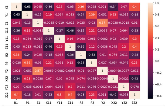
Figure 15.
Correlation matrix for various features.
Furthermore, the correlation between features and the target variable provides insights into feature importance and predictive power, and variables with higher correlations to the target variable may have stronger predictive capabilities, making R1 and P1 more crucial, followed by Z22 and X22, thereby impacting model interpretability and performance. It is essential, however, to remember that correlation does not denote causation, as a high correlation between two variables does not necessarily imply a causal relationship.
4.2. Randomized Convolutional Kernel Transform (ROCKET)
The fast execution time and great accuracy of ROCKET (randomized convolutional kernel transform) in comparison with other state-of-the-art ML models make it a viable option [22].
4.2.1. Hyperparameter Selection
The prominent selection is of the kernel as it uses conventional CNNs with default settings in the beginning for its length, bias, padding, dilation, and, finally, weights. The two kernel choices are made after successively increasing numbers, one with 400 and the other with 450 kernels, considering the computational resources available. The penalization of the linear classifier for complexity in ROCKET is controlled by the “regularization parameter”. A higher value for this regularization parameter can avoid overfitting, but at the same time, the classifier is less accurate. Stride length controls time series application convolutional kernels. Stride and features have an inverse relationship: a higher value of stride will result in fewer features, with the added advantage of a more robust classifier to noise [22].
4.2.2. Performance
For this application, the ROCKET classifier algorithm underperformed, and its description is shown in Table 8 and Table 9, and Figure 16.
Table 8.
ROCKET classifier accuracy for different kernel sizes.
Table 9.
Evaluation metrics for ROCKET classifier.
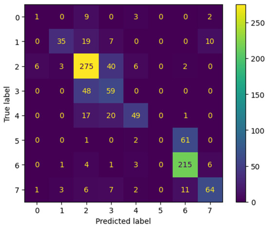
Figure 16.
Confusion matrix for ROCKET classifier.
The imbalance of class inherent to the gait dataset is the possible cause of the reduced accuracy of the model. Further increase in the kernel count does not result in significant improvement, and even though training time is less, this algorithm is not suited for imbalanced classes.
Classification of gait subphase 5 results in absolute failure associated with inherent minimal gait percentage share similar to the time series classifier, only worse.
4.3. K-Neighbor Time Series Classifier (KNTSC)
The K-neighbor time series classifier (KNTSC) is most widely used as a performance benchmark for classification where dynamic time warping is used in conjunction with one nearest neighbor. The Euclidean distance metric is used for this application [23].
Performance
The choice of window size for data input is critical due to the presence of sparsely distributed IMU outputs in certain gait subphase data. When using large windows, noise can be introduced by combining multiple data rows, while small windows may result in significant feature loss. Despite the computational cost, the overall performance remains acceptable. For classes 6 and 7, the features used for training the model might not be sufficiently informative or discriminating, which causes the model to not capture the underlying patterns in the data well, and means that the model might not be able to distinguish between classes effectively. The performance of this classifier is shown in Figure 17, Table 10 and Table 11.

Figure 17.
Confusion matrix for K-nearest neighbor algorithm.
Table 10.
K-neighbor time series classifier accuracy for different neighbor counts.
Table 11.
Evaluation metrics for K-neighbor time series classifier.
4.4. LSTM–FCN Classifier
Karim et al. [24] used a fully convolutional network (FCN) in conjunction with LSTM, which resulted in significant improvement in the time series classification of multivariate data. The major concern with LSTM–FCN architecture (Figure 18 and Table 12) is to have a tradeoff between computational complexity and required accuracy. The number of seven classes is fixed and the length of time series data can be varied. The model has 267,496 parameters, of which 266,472 are trainable and 1024 are nontrainable. They are associated with the convolutional and normalization layers, the weights of which are desired to be pivoted. The model performed better than ROCKET and KNTSC, but the precision and recall for the fifth class were still very poor. The accuracy converged to a value of 0.78, and further change in the LSTM size and other parameters did not result in significant improvement in the results. The large parameters and complex architecture make LSTM–FCN for this application not suitable for deployment. The performance of this classifier is shown in Figure 19, Table 13.
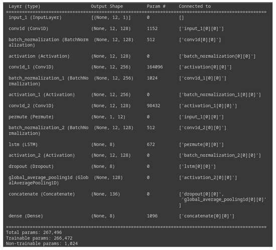
Figure 18.
LSTM–FCN classifier architecture.
Table 12.
LSTM–FCN hyperparameters.
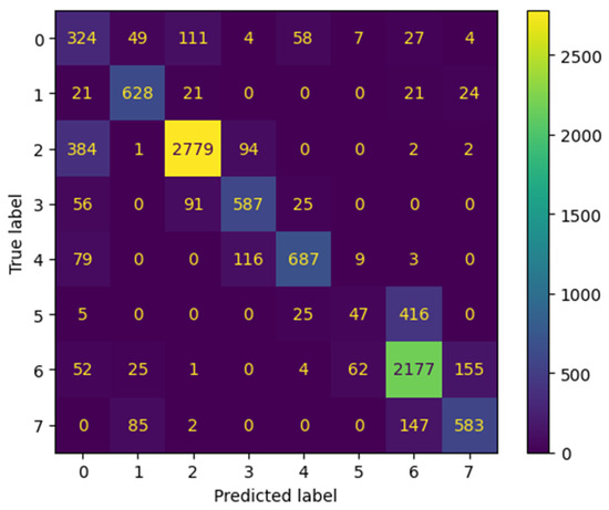
Figure 19.
Confusion matrix for LSTM–FCN classifier.
Table 13.
Evaluation metrics for LSTM–FCN.
Table 14 presents a comprehensive overview of the performance of the time series classifiers. Among them, the time series forest classifier (TSFC) stands out as the most suitable choice for gait identification applications, boasting an impressive accuracy of 0.86. The TSFC classifier exhibits notable precision and recall rates, accompanied by a respectable F1-score, thereby demonstrating its efficacy in accurately classifying gait patterns while minimizing false positive results. It is worth noting that class 5, characterized by the lowest percentage of gait samples at a mere 5%, is associated with a limited number of data samples due to the constrained data transfer baud rate of 115,200. Consequently, the fifth gait class consists of only a small number of samples, typically in the range of tens. This scarcity of data adversely affects the classification performance, as evidenced by the ROCKET and K-NTSC classifiers, both of which yield absolute scores of 0 for precision, recall, and F1-score. Consequently, these classifiers are deemed unsuitable for practical usage. The misclassification of class 5 in random forest to class 6 could be potentially tolerated for system deployment, as the difference in the activation level of knee moment associated with these two for normalized value is 0.026, obtained from Table 5.
Table 14.
Performance metrics for classifiers.
Comparing LSTM–FCN and TSFC, it is evident that TSFC achieves higher performance scores and exhibits computational feasibility during training, as well as ease of deployment. However, in class 0, which encompasses non-gait-related data such as stationary conditions and abnormal activities, LSTM–FCN slightly outperforms TSFC. This marginal advantage of LSTM–FCN in class 0 can be attributed to its enhanced ability to extract relevant features from the data.
A single gait cycle typically has an average duration of 0.98 to 1.02 s. Phase 5 therefore averages approximately 50 milliseconds. Given the computations performed by the IMU and the limited 115,200 baud rate for UART data transfer, the output data range from 2 to 15 data points per gait cycle. This imbalanced dataset cannot be equalized using conventional methods such as undersampling, oversampling, or ensembling. Therefore, class weighting is applied by assigning a higher weight to the class with fewer samples. Precision, recall, F1-score, and weighted average are used as performance metrics due to this imbalanced distribution.
A knee orthosis brace assisted by a magnetorheological brake had been published in our previous research [25], for which the gait phase identification and activation was proposed. The orthosis has a metallic structure for the orthosis, and the flexion joint is modified to house a reduction gear mechanism coupled with an MR brake.
5. Conclusions
This study focuses on developing a machine-learning-based gait phase identification methodology for flexion damping marked with simulated knee moment. The methodology utilizes IMU data collected from two Adafruit BNO085 sensors placed on the thigh and shin. Foot switches are used for data acquisition and labeling, facilitating the capture of activation patterns aligned with a normal gait. OpenSim, an open-source musculoskeletal simulation software, is utilized for simulation using existing experimental gait motion-capture data and reaction force data.
Inverse kinematic and inverse dynamic simulations are applied to derive important metrics such as knee joint angle and knee moment, which are then normalized and scaled. The synchronization of IMU and foot switch data through meticulous data capture methodology enables the creation of comprehensive labeled subphase datasets. By integrating simulation results with these datasets, activation data for knee flexion dampening are obtained. Multiple supervised machine learning algorithms are trained and evaluated, with the time series forest classifier displaying the most robust performance.
The work classifies the gait phases into seven different classes, as defined in Table 3. In future work, the number of classes can be expanded by incorporating a pressure sensor instead of a binary switch for phase segregation. Additionally, utilizing signal analysis techniques such as thresholding and min–max cutoff can further segment the classes into smaller portions. The current method employs a fixed activation level for each class, derived from simulation. This necessitates the use of a smoothing function to transform the output activation values from step signals to transient curves. However, this smoothing process reduces the resolution of the activation signal. To address this issue, the same simulation results can be applied with an increased number of classes, allowing for more precise validation of the activation magnitude through moment output.
Furthermore, it should be noted that the overall accuracy of the time series forest is 86%, which may be insufficient for applications requiring more accurate predictions, such as gait abnormality detection. Additional training for abnormal gaits might be necessary. Notably, the gait phase associated with class 5 is of particular interest, as it appears to be a bottleneck in the existing hardware setup. The computation time is predominantly consumed by the motion engine of the IMUs performing sensor fusion, resulting in an imbalanced dataset and poor predictability. It is worth highlighting that the activation of the median right knee moment does not vary significantly between classes 5 and 6, ranging from 0.580 to 0.599. Subsequent research should focus on enhancing data collection resolution by increasing the number of IMUs and exploring alternative methods for marking gait subphases. Furthermore, a wider array of machine learning models should be investigated. Practical implementation considerations include the deployment of an edge computer with a well-designed controller system to facilitate real-world applications. In rehabilitation contexts, utilizing the variable braking capability of the MR brake can optimize the rehabilitative process by gradually augmenting the brake profile based on each patient’s recovery progress.
Author Contributions
Conceptualization, Y.S.; methodology, Y.S. and R.B.; software, R.B.; validation, Y.S. and R.B.; formal analysis, Y.S. and R.B.; investigation, R.B.; data curation, R.B.; writing—original draft preparation, R.B.; writing—review and editing, Y.S.; supervision, Y.S.; project administration, Y.S.; funding acquisition, Y.S. All authors have read and agreed to the published version of the manuscript.
Funding
This research was funded by the Ministry of Science and Technology (MOST), Taiwan, grant number 109-2221-E-027-048.
Institutional Review Board Statement
Ethical review and approval were waived for this study, due to all subjects involved in this study being authors or lab members.
Informed Consent Statement
Written informed consent was obtained from all subjects to publish this paper.
Data Availability Statement
Not applicable.
Conflicts of Interest
The authors declare no conflict of interest.
References
- Bortoluzzi, A.; Furini, F.; Scirè, C.A. Osteoarthritis and its management—Epidemiology, nutritional aspects and environmental factors. Autoimmun. Rev. 2018, 17, 1097–1104. [Google Scholar] [CrossRef] [PubMed]
- Vaughan, C.L.; Davis, B.L.; O’Connor, J.C. Dynamics of Human Gait, 2nd ed.; Kiboho: Cape Town, South Africa, 1999. [Google Scholar]
- Silva, H.; Júnior, A.; Zorzi, A.; Miranda, J. Biomechanical changes in gait of subjects with medial knee osteoarthritis. Acta Ortop. Bras. 2012, 20, 150. [Google Scholar] [CrossRef] [PubMed]
- Arteaga, O.; Terán, H.C.; Morales, H.; Argüello, E.; Erazo, M.I.; Ortiz, M.; Morales, J.J. Design of Human Knee Smart Prosthesis with Active Torque Control. Int. J. Mech. Eng. Robot. Res. 2020, 9, 347–352. [Google Scholar] [CrossRef]
- Jiankang, H.; Dichen, L.; Bingheng, L.; Zhen, W.; Tao, Z. Custom fabrication of composite tibial hemi-knee joint combining CAD/CAE/CAM techniques. Proc. Inst. Mech. Eng. Part H J. Eng. Med. 2006, 220, 823–830. [Google Scholar] [CrossRef] [PubMed]
- Teng, H.; Calixto, N.; MacLeod, T.; Nardo, L.; Link, T.; Majumdar, S.; Souza, R. Associations between patellofemoral joint cartilage T1ρ and T2 and knee flexion moment and impulse during gait in individuals with and without patellofemoral joint osteoarthritis. Osteoarthr. Cartil. 2016, 24, 1554–1564. [Google Scholar] [CrossRef] [PubMed]
- Bishop, C.M. Pattern Recognition and Machine Learning; Springer: New York, NY, USA, 2006. [Google Scholar]
- Kreuzer, D.; Munz, M. Deep Convolutional and LSTM Networks on Multi-Channel Time Series Data for Gait Phase Recognition. Sensors 2021, 21, 789. [Google Scholar] [CrossRef] [PubMed]
- Prakash, C.; Gupta, K.; Kumar, R.; Mittal, N. Fuzzy Logic-Based Gait Phase Detection Using Passive Markers; Springer: Singapore, 2016; pp. 561–572. [Google Scholar] [CrossRef]
- Taborri, J.; Rossi, S.; Palermo, E.; Cappa, P. A HMM distributed classifier to control robotic knee module of an active orthosis. In Proceedings of the 2015 IEEE International Conference on Rehabilitation Robotics (ICORR), Singapore, 11–14 August 2015; pp. 277–282. [Google Scholar] [CrossRef]
- Delp, S.L.; Anderson, F.C.; Arnold, A.S.; Loan, P.; Habib, A.; John, C.T.; Guendelman, E.; Thelen, D.G. OpenSim: Open-source software to create and analyze dynamic simulations of movement. IEEE Trans. Bio-Med. Eng. 2007, 54, 1940–1950. [Google Scholar] [CrossRef] [PubMed]
- Seth, A.; Anderson, F.C. Gait 2392 and 2354 Models. 2017. Available online: https://simtk-confluence.stanford.edu:8443/display/OpenSim/Gait+2392+and+2354+Models (accessed on 1 April 2023).
- John, C.T.; Anderson, F.C.; Higginson, J.S.; Delp, S.L. Stabilisation of walking by intrinsic muscle properties revealed in a three-dimensional muscle-driven simulation. Comput. Methods Biomech. Biomed. Eng. 2013, 16, 451–462. [Google Scholar] [CrossRef] [PubMed]
- Kuo, A.D. A least-squares estimation approach to improving the precision of inverse dynamics computations. J. Biomech. Eng. 1998, 120, 148–159. [Google Scholar] [CrossRef] [PubMed]
- Murray, M.P.; Drought, A.B.; Kory, R.C. Walking patterns of normal men. J. Bone Jt. Surg. 1964, 46, 335–360. [Google Scholar] [CrossRef]
- Löning, M.; Bagnall, A.; Ganesh, S.; Kazakov, V.; Lines, J.; Király, F.J. Sktime: A Unified Interface for Machine Learning with Time Series. arXiv 2019, arXiv:1909.07872. [Google Scholar]
- Löning, M.; Király, F.; Bagnall, T.; Middlehurst, M.; Ganesh, S.; Oastler, G.; Lines, J.; Walter, M.; ViktorKaz; Mentel, L.; et al. Sktime/Sktime: V0.13.4 (V0.13.4). Zenodo. 2022. Available online: https://zenodo.org/record/7117735 (accessed on 25 April 2023).
- Kane, M.; Price, N.; Scotch, M.; Rabinowitz, P. Comparison of ARIMA and Random Forest time series models for prediction of avian influenza H5N1 outbreaks. BMC Bioinform. 2014, 15, 276. [Google Scholar] [CrossRef]
- Liu, H.; Wu, H.; Yu, C. A hybrid model for appliance classification based on time series features. Energy Build. 2019, 196, 112–123. [Google Scholar] [CrossRef]
- Breiman, L.; Cutler, A. Random Forests; Chapman and Hall/CRC: Boca Raton, FL, USA, 2001. [Google Scholar]
- Deng, H.; Runger, G.; Tuv, E.; Vladimir, V. A Time Series Forest for Classification and Feature Extraction. Inf. Sci. 2013, 239, 142–153. [Google Scholar] [CrossRef]
- Dempster, A.; Petitjean, F.; Webb, G.I. ROCKET: Exceptionally fast and accurate time series classification using random convolutional kernels. Data Min. Knowl. Discov. 2020, 34, 1454–1495. [Google Scholar] [CrossRef]
- Oehmcke, S.; Zielinski, O.; Kramer, O. kNN ensembles with penalized DTW for multivariate time series imputation. In Proceedings of the 2016 International Joint Conference on Neural Networks (IJCNN), Vancouver, BC, Canada, 24–29 July 2016; pp. 2774–2781. [Google Scholar] [CrossRef]
- Karim, F.; Majumdar, S.; Darabi, H.; Harford, S. Multivariate LSTM-FCNs for Time Series Classification. Neural Netw. 2019, 116, 237–245. [Google Scholar] [CrossRef] [PubMed]
- Kantipudi, M.; Shiao, Y.; Hoang, T. Development of a Multilayer Magnetorheological Brake for Knee orthosis Applications. J. CSME 2021, 42, 81–91. [Google Scholar]


Disclaimer/Publisher’s Note: The statements, opinions and data contained in all publications are solely those of the individual author(s) and contributor(s) and not of MDPI and/or the editor(s). MDPI and/or the editor(s) disclaim responsibility for any injury to people or property resulting from any ideas, methods, instructions or products referred to in the content. |
© 2023 by the authors. Licensee MDPI, Basel, Switzerland. This article is an open access article distributed under the terms and conditions of the Creative Commons Attribution (CC BY) license (https://creativecommons.org/licenses/by/4.0/).