Node2Node: Self-Supervised Cardiac Diffusion Tensor Image Denoising Method

Abstract

Although the existing cardiac diffusion tensor imaging (DTI) denoising methods have achieved promising results, most of them are dependent on the number of diffusion gradient directions, noise distributions, and noise levels. To address these issues, we propose a novel self-supervised cardiac DTI denoising network, Node2Node, which firstly expresses the diffusion-weighted (DW) image volumes along different directions as a graph, then the graph framelet transform (GFT) is implemented to map the DW signals into the GFT coefficients at different spectral bands, allowing us to accurately match the DW image pairs. After that, using the matched image pairs as input and target, a ResNet-like network is used to denoise in a self-supervised manner. In addition, a novel edge-aware loss based on pooling operation is proposed to retain the edge. Through comparison with several state-of-the-art methods on synthetic, ex vivo porcine, and in vivo human cardiac DTI datasets, we showed that the root mean square error (RMSE) of DW images and the average angular error (AAE) of fiber orientations obtained using Node2Node are the smallest, improved by 47.5% and 23.7%, respectively, on the synthetic dataset, demonstrating that Node2Node is not sensitive to the properties of the dataset.

1. Introduction

Heart disease is currently one of the most critical problems that greatly influence human health [1]. Previous studies have shown that the myocardial fiber structure is closely related to the systolic, diastolic, and electromechanical functions of the heart [2,3]. Cardiac fiber disarray usually appears in the early stage of many cardiomyopathies [4]. Therefore, investigating the myocardial fiber structure is of great significance for understanding the causes of various cardiovascular diseases and potentially promoting their early diagnosis. At present, diffusion tensor imaging (DTI) is usually used for mapping the structure of fibrous tissues, which is currently the most promising method to elucidate in vivo myocardium structures non-invasively. However, due to the long acquisition time and the sensitivity of diffusion-weighted (DW) image signals to cardiac or breath motion, the acquired DW images are usually disrupted by the noise, which greatly influences the estimation accuracy of the cardiac fiber structure.

To deal with the effects of noise on DW images, numerous post-processing methods have been proposed. The early DW image denoising methods are based on spatial filters [5,6], edge regularizations [7,8], sparse regularizations [9,10], or prior information [11,12,13], such as adaptive smoothing methods, sparse dictionary-based methods, non-local means, Bayesian methods, etc. These traditional methods require manually setting many hyperparameters; in addition, they need to be optimized for each DW image individually, which is time-consuming and not stable. Accordingly, they are prone to introducing errors in the subsequent analysis regarding diffusion metrics. To address these problems, according to the nature of DW image volumes, noise removing methods based on four-dimensional (4D) DW images have been proposed. For instance, Manjón et al. proposed an adaptive optimized non-local means (AONLM) [14], which fully considered the spatially or directionally varied noise level in DW images, and designed an adaptive noise filter according to the similarity of the local blocks. Subsequently, the authors presented another local principal component analysis (LPCA) method [15], which fully exploited the multidirectional redundancy of DW images, and used the thresholded principal component decompositions of each 4D local block to remove the noise in DW images. Recently, Fadnavis et al. proposed a novel method, Patch2Self [16], which approximated the clean signal of a single DW image voxel from the noisy DW signals of several small local patches around this voxel along different directions through linear regression. Since the random noise cannot be linearly fitted, Patch2Self can achieve better noise reduction performance on a variety of diffusion datasets. Even though the above-mentioned methods can deal with the spatially or directionally varying non-Gaussian noise in DW images, many of them are sensitive to the number of diffusion directions. When the number of diffusion directions is not sufficient, the performance of these methods decreases dramatically.

Recently, emerging convolutional neural networks (CNNs) have provided another promising alternative for medical image denoising. Using the supervised CNN models can easily restore the noise-free images from the noisy observations by fully exploring the redundancy embedded in large image datasets. For instance, Zhang et al. proposed a denoising convolutional neural network (DnCNN) [17] which can achieve a better performance than traditional block matching and 3D collaborative filtering (BM3D) denoising methods [18] with an extremely simple architecture. Currently, CNN-based denoising methods have been widely used in X-ray [19], PET [20,21], CT [22,23], and MRI images [24]. Regarding DW images, Wang et al. first proposed a joint denoising CNN (JD-CNN) model which can effectively reduce noise by taking multiple b-value DW images as the multichannel input of the network [25]. Subsequently, the DeepDTI model was proposed [26], which leverages a 3D CNN to denoise DW image volumes along six optimally selected diffusion directions. For providing a target to train the network in a supervised manner, numerous noise-free DW images are synthesized from the given tensors. DeepDTI can not only be used to denoise but also to accelerate DTI reconstruction since it uses only six directions.

Despite the superior performance of these supervised learning-based methods, their requirement for additional noise-free images or large amounts of SNR data makes them difficult to use in clinical applications. In one aspect, large amount of noise-free images or large amounts of SNR data are almost unavailable; in the other aspect, well-trained CNNs are usually not generalized, so they cannot adapt well to new data with different image contrasts, noise levels, spatial resolutions, etc. Accordingly, this prohibits the real clinical applications of a supervised model. To address these challenges, unsupervised or self-supervised learning-based denoising methods have emerged. For instance, Lin et al. used a deep image prior (DIP) model to denoise multiple b-value DW images [27]. It assumes that with some given network parameters, the output of the network can represent noise-free images. This is considered to be the prior of the deep network. Due to this assumption, the denoising performance of DIP is dependent on the iteration times. In other words, for DW images with different b-values or different diffusion gradient directions, the optimal iteration times will change since the optimal parameters for different DW images are totally different. This increases the difficulty in optimization; in addition, stability in the denoising performance cannot be guaranteed. Based on DeepDTI, the authors present another DTI denoising model, SDnDTI [28]. Instead of using synthesized clean data as the learning targets, SDnDTI uses the average of multiple repetitions of the synthesized noisy DW images as the target. This operation allows the model to train using its self-information rather than the additional ground-truth. Besides the models focused on DW images, there are numerous models that use self-information to denoise the natural images, such as Noise2Noise [29], Neighbor2Neighbor [30], Noise2Void [31], Noise2Self [32], Self2Self [33], etc. The key of these methods is to generate similar image or block pairs from the noisy image-self, and to take them as the input and target of a learning network, respectively, to denoise. For instance, Noise2Noise uses two noisy observations of the same scene obtained at different times as the input and target; in Neighbor2Neighbor, the adjacent image patches in one noisy image are taken as the input and target; and Self2Self it uses Bernoulli dropout sampling to form the input and target image pairs. These self-supervised learning-based denoising methods cannot directly be used on DW images since they do not consider the relationships among the DW images along different directions, which may cause problems for the subsequent diffusion tensor reconstruction. To solve this problem, recently, a structural-similarity-based convolutional neural network with edge-weighted loss (SSECNN) was proposed by Yuan et al. [34]. It explores the self-similarity in DW images along different directions to denoise, achieving promising results. However, the similarity between the noisy directional DW images in SSECNN was calculated with a structural similarity index (SSIM), which is very sensitive to noise and may introduce bias in similar image pair matching, therefore influencing its denoising performance.

To address this issue, we propose a novel self-supervised cardiac DW image denoising network, Node2Node, which uses graph framelet transform (GFT) [35] to divide the DW signals into different sub-bands, allowing it to more accurately search the similar DW image pairs in a band-to-band manner. Specifically, in view of q-space, DW image volume along one diffusion direction can be taken as a node in q-space, with the DW images being the features of the node. Accordingly, we first express the DW image volumes along different directions as a graph; then, the GFT is implemented on the graph to map the DW signals into the coefficients at different spectral bands. By computing the coefficients’ similarities at different bands, the influence of the noise on the similar DW image pair matching can be decreased. After that, using the matched image pairs as input and target, respectively, a ResNet-like network architecture is used to denoise. In addition, to avoid the over-smooth phenomenon, a novel edge-aware loss based on dilation and erosion (realized by pooling operations) is proposed. It can adaptively adjust the loss weights on edge and smooth regions to improve the further denoising performance.

2. Methods

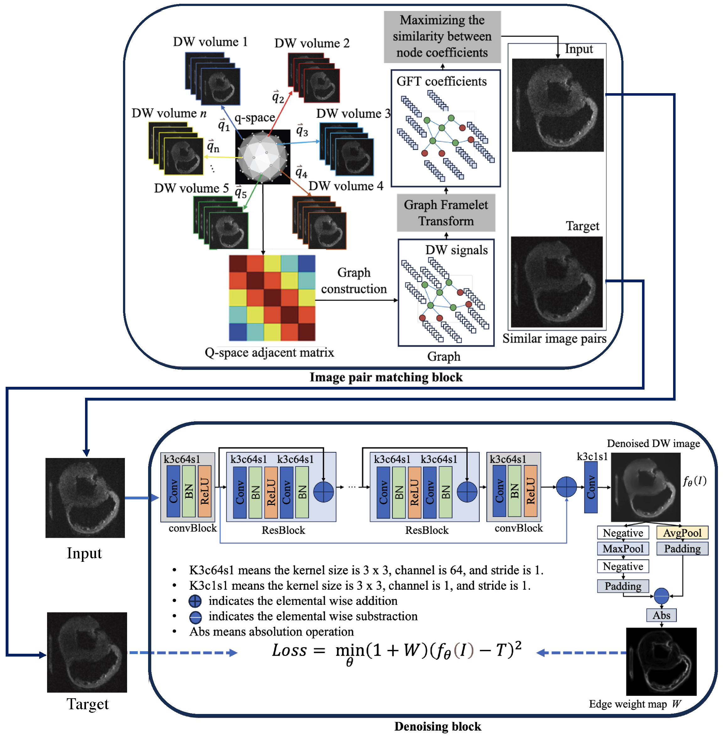
2.1. The Overall Structure of the Node2Node Network

In DTI, the DW images are acquired from the multiple diffusion gradient directions which are uniformly sampled from the q-space. In view of q-space, each diffusion direction can be taken as a node and the similarity between the different directions can be considered the adjacent matrix between nodes. Accordingly, the DW images along different directions can be expressed in a graph, with the DW signals (reshaped DW image volume along one direction into a vector) being the node features. Considering that the DW images acquired from the adjacent diffusion gradient directions are similar, and the noise in DW images along different directions has the same distribution, this work proposes a novel self-supervised cardiac DW image denoising network, Node2Node. Its architecture is illustrated in Figure 1, consisting of a noisy-image pair matching block realized with graph framelet transform, and a denoising block based on ResNet.

The detailed process of the noisy DW image pair matching is elaborated as follows. Firstly, according to the diffusion gradient directions $\overrightarrow{q}$, we construct a q-space graph. Considering that in the cardiac DTI, all the DW images are acquired with the same b value, accordingly, during the q-space graph construction, only the diffusion directions are used. Specifically, each direction is considered a graph node, and the adjacent coefficient between two nodes is defined as:

$$c_{i,j}=exp(-\frac{1-{\left({{\overrightarrow{q}}_i}^T{\overrightarrow{q}}_j\right)}^2}{2{\sigma }_q^2})i,j=1,2,\cdots ,N$$

(1)

where ${\overrightarrow{q}}_i$ and ${\overrightarrow{q}}_j$ represent the $i_{th}$ and $j_{th}$ diffusion directions, ${\sigma }_q$ indicates a hyperparameter to control the adjacent coefficient $c_{i,j}$ between ${\overrightarrow{q}}_i$ and ${\overrightarrow{q}}_j$, and N is the total number of diffusion directions.

Based on $c_{i,j}$, the adjacent matrix A and degree matrix D of the q-space graph can be derived,  

$$\begin{array}{cc}\hfill A_{i,j}& =c_{i,j}i,j=1,2,\cdots ,N\hfill \\ \hfill D_i& =\sum _{j=1,j\ne i}^n{c}_{i,j}.\hfill \end{array}$$

(2)

Graph framelet transform is a filter method that is implemented on the graph spectral domain for dividing the signal into different sub-bands, which allows us to more accurately evaluate the feature similarity between the nodes in a band-to-band manner. In this work, GFT is implemented on the q-space graph $G=(V,E)$. In other words, in graph G, the vertex V represents the features of nodes. In this work, they are the DW images or signals acquired from a certain direction, and E indicates the edge between the nodes which is determined by the values of the adjacent matrix. According to the convolution theory, the convolution (filter) in spatial space corresponds to the point-wise product in spectral space. Assuming that the filter in spatial space is h, and the spatial signal is s, the filtering result can be expressed as:

$$h\ast s={\mathcal{FFT}}^{-1}(\mathcal{FFT}\left(h\right)\odot \mathcal{FFT}\left(s\right))$$

(3)

where $\mathcal{FFT}$ and ${\mathcal{FFT}}^{-1}$ represent the Fourier and inverse Fourier transform, respectively, ⊙ indicates the point-wise product. Since GFT is performed on the graph in the spectral domain, we should derive the Fourier and inverse Fourier transform of the graph signal. The Fourier transform basis of a graph G is defined as the eigenvectors of the Laplacian matrix L of graph G. Given the adjacent matrix and degree matrix, the Laplacian matrix of a graph is derived by $L=D-A$. Through the eigen-decomposition of matrix L, the pairs of eigenvalues and eigenvectors of L are derived, denoted as ${\{{\lambda }_k,u_k\}}_{k=0}^{N-1}$. The eigenvectors form the orthogonal basis $U=[u_0,u_2,\cdots ,u_{N-1}]$ for performing the Fourier transform on the graph, meaning that the filter operation on the graph can be rewritten as:

$$\begin{array}{cc}\hfill h\ast s& =U(U^{T}h\odot U^{T}s)=U\mathrm{diag}\left(\widehat{h}\right)U^{T}s\hfill \\ \hfill & =U\mathrm{diag}({\widehat{h}}_0,{\widehat{h}}_1,\cdots ,{\widehat{h}}_{N-1})U^{T}s\hfill \end{array}$$

(4)

where $\widehat{h}$ means the transformed filter of h, with ${\widehat{h}}_0$ representing the low-pass filter, and ${\widehat{h}}_1,{\widehat{h}}_2,\cdots ,{\widehat{h}}_{N-1}$ are the band-pass and high-pass filters; diag $(·)$ indicates the diagonalization operation. Designing filter h is equal to determining the multipliers ${\widehat{h}}_0,{\widehat{h}}_1,\cdots ,{\widehat{h}}_{N-1}$ in the spectral domain. In this work, these filters are designed with GFT, meaning that $\mathrm{diag}(\widehat{h})={\widehat{H}}_r\left(c_l\right)$, expressed as: 

$$\begin{array}{cc}\hfill {\widehat{H}}_r\left(c_l\right)& ={\mathrm{\Omega }}_r\left(c_l\tilde{\mathrm{\Lambda }}\right)l=1\hfill \\ \hfill {\widehat{H}}_r\left(c_l\right)& ={\mathrm{\Omega }}_r\left(c_l\tilde{\mathrm{\Lambda }}\right)\prod _{l^{\prime }=1}^{l-1}{\mathrm{\Omega }}_0\left(c_{l^{\prime }}\tilde{\mathrm{\Lambda }}\right)2\le l\le Lev\hfill \end{array}$$

(5)

where $l=1,2,\cdots ,Lev$ means the decomposition level of GFT, $r=0,1,\cdots ,R$ indicates the index of the frequency band, $r=0$ indicates the low-pass filter, and the others are band-pass and high-pass filters. $\tilde{\mathrm{\Lambda }}=\mathrm{diag}\{{\tilde{\lambda }}_0,{\tilde{\lambda }}_1,\cdots ,{\tilde{\lambda }}_{N-1}\}$ with ${\tilde{\lambda }}_k={\lambda }_k/{\lambda }_{max}\pi$, $c_l$ is the scale function defined by $c_l={\gamma }^{-Lev+l}$, with $\gamma >1$ being a scale factor. The matrix $\mathrm{\Omega }\left(c_l\tilde{\mathrm{\Lambda }}\right)$ is defined by:  

$${\mathrm{\Omega }}_r\left(c_l\tilde{\mathrm{\Lambda }}\right)=\mathrm{diag}\{{\widehat{\alpha }}_r\left(c_l{\tilde{\lambda }}_0\right),{\widehat{\alpha }}_r\left(c_l{\tilde{\lambda }}_1\right),\dots ,{\widehat{\alpha }}_r\left(c_l{\tilde{\lambda }}_{N-1}\right)\}$$

(6)

in which ${\widehat{\alpha }}_r(·)$ is the framelet filter. In this work, ${\widehat{\alpha }}_r(·)$ is implemented with Haar wavelet, meaning that $R=1$ and ${\widehat{\alpha }}_r\left(x\right)$ is formulated as:

$$\begin{array}{c}\hfill {\widehat{\alpha }}_0\left(x\right)=cos(x/2)\\ \hfill {\widehat{\alpha }}_1\left(x\right)=sin(x/2).\end{array}$$

(7)

With the spectral filters ${\tilde{H}}_r\left(c_l\right)$, the GFT coefficients of the signal s can be written as:

$${\varphi }_s={\tilde{H}}_r\left(c_l\right)U^{T}s.$$

(8)

Denoting the DW image signal at the node i and j as $s_i$ and $s_j$, respectively, the corresponding GFT coefficients can be calculated with Equation (8) and noted as ${\varphi }_{s_i}$ and ${\varphi }_{s_j}$. To find the matched DW image pair with GFT coefficients, the similarity $w_{ij}$ between ${\varphi }_{s_i}$ and ${\varphi }_{s_j}$ is calculated with:

$$\begin{array}{cc}\hfill w_{ij}& =\frac{1}{Z_i}exp\left(-\frac{{∥{\varphi }_{s_i}-{\varphi }_{s_j}∥}_2^2}{2\beta {\left({\sigma }_{GFT}\right)}^{2}d}\right)\hfill \\ \hfill Z_i& =\sum _{j=0}^{N-1}exp\left(-\frac{{∥{\varphi }_{s_i}-{\varphi }_{s_j}∥}_2^2}{2\beta {\left({\sigma }_{GFT}\right)}^{2}d}\right)\hfill \end{array}$$

(9)

where $\beta$ and ${\sigma }_{GFT}$ are hyperparameters and d is the dimension of ${\varphi }_{s_i}$. For any DW image at node i, we find the DW image at node j with the biggest similarity $w_{ij}$ to form the noisy image pairs $\{I_i,I_j\}$. The process of DW image pair matching is detailed in Algorithm 1.

According to the idea of the Noise2Noise, taking $I_i$ as the input of a denoising network and $I_j$ as the learning target, the well-trained network can be used to remove the noise. In this work, the baseline of the denoising network is ResNet, which consists of a convBlock (Conv + BatchNorm + ReLU), 16 residual blocks, and a convBlock as well as a convolutional layer (as illustrated in Figure 1). The convolution kernel size in all the blocks is 3, stride = 1, and padding = 1.

Algorithm 1 DW noisy image pair matching algorithm

Require:    ${\overrightarrow{q}}_i$: the ith diffusion gradient direction, $i=1,2,\cdots ,n$, n is the number of directions.    $I_i$: the DW image along ith diffusion direction    ${\sigma }_q$, ${\sigma }_{GFT}$, $\beta$: the hand-crafted hyper-parameters Step1: according to Equations (1) and (2) to calculate the adjacent matrix of graph G, reshaping DW images along the ith diffusion direction as a DW signal vector $s_i$ and noting it as the features of the node i. Step2: calculating the Laplacian matrix L of graph G and implementing eigen-decomposition on L to derive the Fourier basis U. Step3: deriving the graph framelet transform coefficients ${\varphi }_{s_i}$ for the features of each node based on the Equations (5)–(8). Step4: for the ith node, finding the most similar node j from the rest nodes by maximizing the similarity between ${\varphi }_{s_i}$ and ${\varphi }_{s_j}$ with Equation (9). return the DW images along ith and jth directions $I_i$ and $I_j$.

2.2. Loss Functions

Since the idea of Node2Node is similar to that of Noise2Noise, we also use the MSE loss between $f_{\theta }\left(I_i\right)$ and $I_j$ to train the network, where $f_{\theta }$ represents the nonlinear function expressed by the network with $\theta$ being the network parameters. The loss can be formulated as:

$$Loss=\underset{\theta }{argmin}{(f_{\theta }\left(I_i\right)-I_j)}^2$$

(10)

Considering that MSE loss is prone to over-smoothing the denoised image, to address this issue, we propose an edge-aware loss implemented with erosion and dilation operation through max-pooling and average pooling, detailed as:

$$W_{edge}=\frac{|AvgPool\left(f_{\theta }\left(I_i\right)\right)+MaxPool(-f_{\theta }\left(I_i\right))|}{Max\left(\right|AvgPool\left(f_{\theta }\left(I_i\right)\right)+MaxPool(-f_{\theta }\left(I_i\right))\left|\right)}$$

(11)

where $| · |$ indicates the absolute and Max the maximum value. $AvgPool\left(x\right)$ can dilate the image x, while $-MaxPool(-x)$ can erode the image x and using $AvgPool\left(x\right)-(-MaxPool(x\left)\right)$ can emphasize the image edges. Therefore, the normalized edge weight is designed like Equation (11). To retain the edge details during the denoising, we propose an edge-aware loss that be written as:

$$Los{s}_w=(1+W_{edge})Loss.$$

(12)

This allows the model to adjust the loss weights on different regions.

3. Experiments

3.1. Datasets

One synthetic dataset and two public available real datasets were used in this work to evaluate the proposed method.

(1)

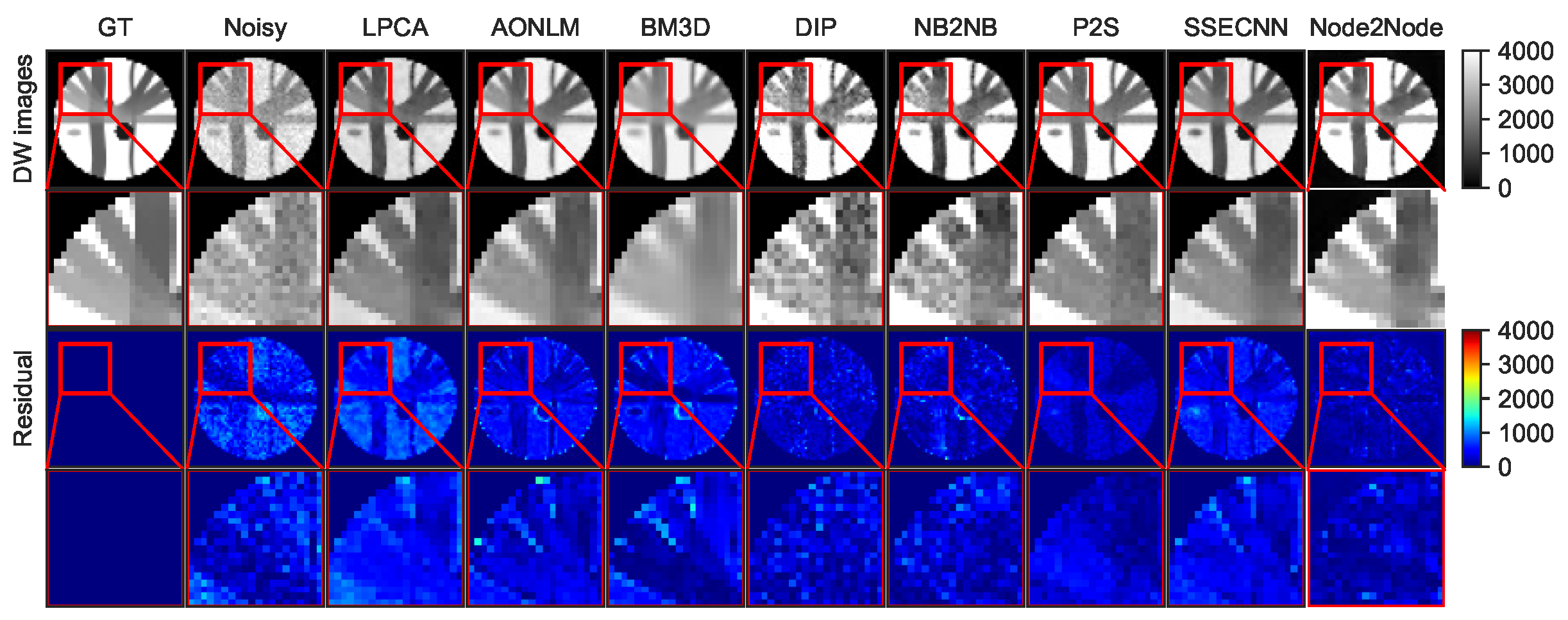
Synthetic data: To quantitatively evaluate the performance of the proposed denoising method, we synthesized noise-free DW images using Phantom$\mathsf{\alpha }$s (http://www.emmanuelcaruyer.com/phantomas.php, accessed on 12 December 2021). with a b-value of 1000 s/mm${}^2$ and six diffusion gradient directions. The fiber structure setting is the same as that used in the ISBI 2013 HARDI challenge. The DW image size is $55\times 55\times 55$, and the spatial resolution is $1.5\times 1.5\times 1.5$ mm${}^3$. To obtain the noisy images, random Gaussian noise with level of 10% was added to the clean image five times, resulting in a total of 1650 noisy DW images.

(2)

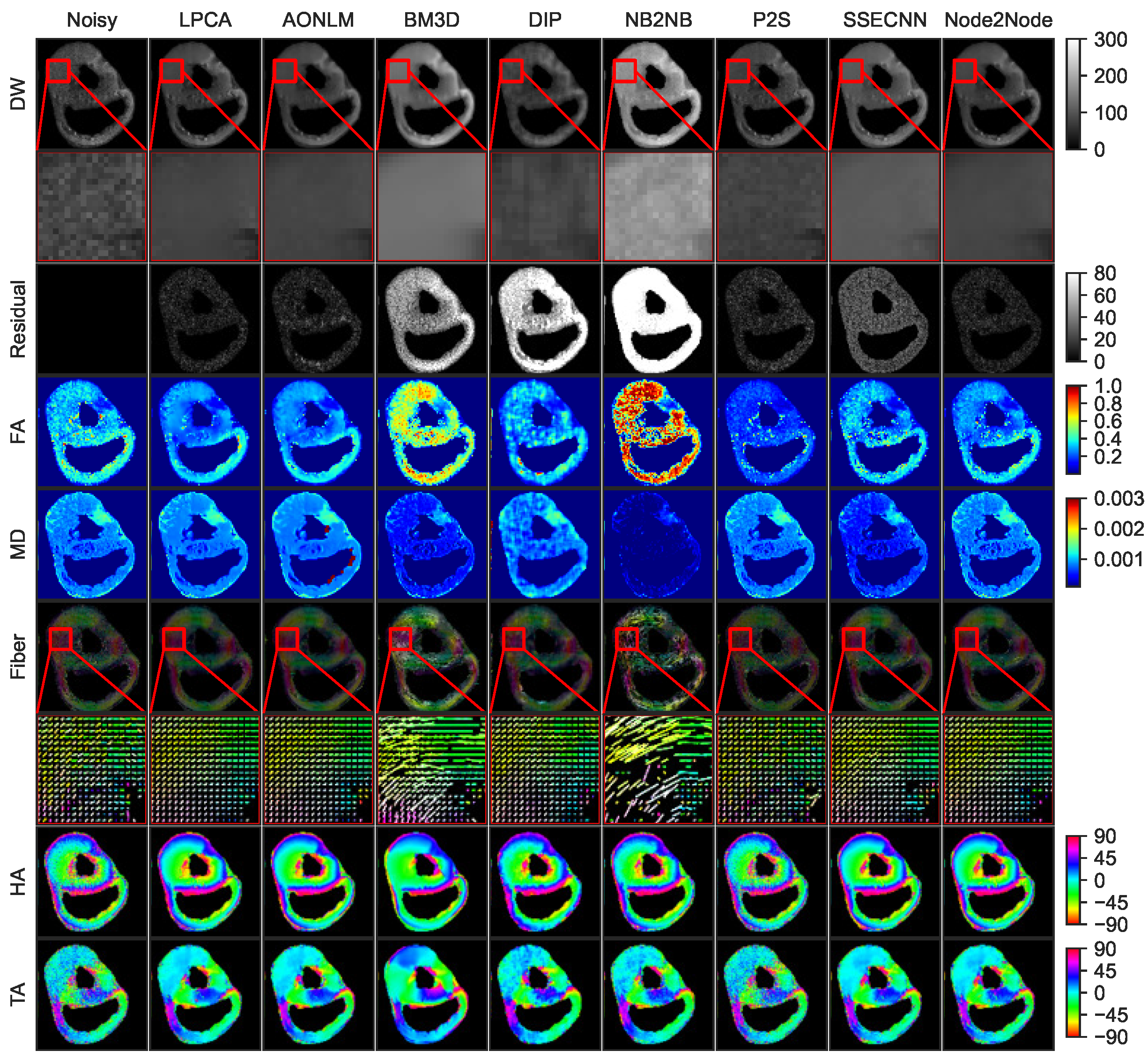
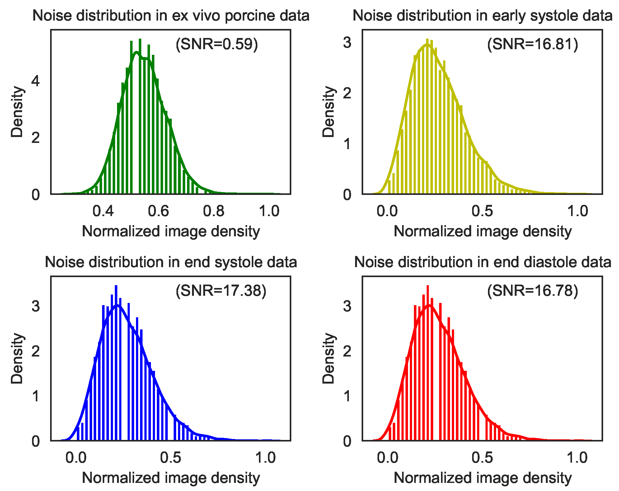
Ex vivo porcine cardiac DTI data: This dataset was provided by the cardiac MRI research (CMR) group at Stanford University (https://med.stanford.edu/cmrgroup/data/ex_vivo_dt_mri.html, accessed on 22 November 2022). It comprises seven ex vivo porcine hearts that were imaged using a SIEMENS Prisma_fit scanner with a diffusion sequence, TE = 58 ms, TR = 16,670 ms, and 30 diffusion gradient directions with b-value of 1000 s/mm${}^2$, conducted five times. The image spatial resolution is $1\times 1\times 1$ mm${}^3$, and the image size is $128\times 128\times 120$. That means that there are a total of 126,000 DW images in this dataset.

(3)

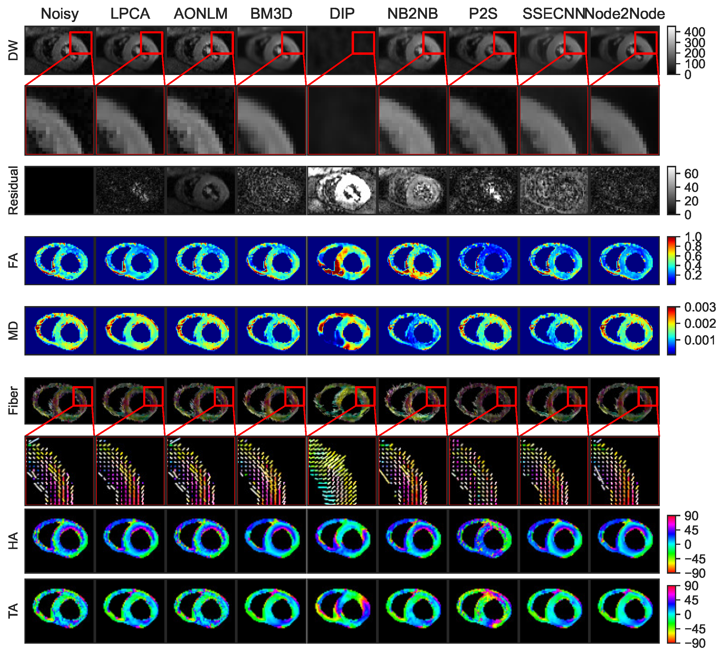
In vivo human cardiac DTI data at multiple cardiac phases: This in vivo human cardiac DTI dataset was also provided by Standord University (https://med.stanford.edu/cmrgroup/data/myofiber_data.html, accessed on 30 June 2023). It contains the cardiac DW images of nine healthy volunteers acquired using a 3T MRI scanner (Prisma, Siemens) and a single-shot spin EPI sequence incorporated with second-order (M1–M2) motion-compensated gradient. For each subject, only one mid-ventricular short-axis slice was imaged at early systole, end systole, and end diastole phases, respectively. The acquisition parameters are: TE = 61 ms, matrix size = 128 × 104, in-plane resolution = $1.6\times 1.6$ mm${}^2$, slice thickness = 8 mm, b-value = 350 s/mm${}^2$, and number of diffusion gradient directions = 12. Each subject was scanned eight times, meaning a total of 96 DW images were acquired per cardiac phase. In total, there are 864 images in this dataset.

3.2. Experimental Implementations

To demonstrate the superiority of the proposed method, we compare it with several typical DW image denoising methods, including LPCA, AONLM, and BM3D, as well as some learning-based methods, such as DIP, Neighbor2Neighbor (NB2NB), patch2Self (P2S), and SSECNN. All the typical comparison methods kept their default settings, and the learning-based methods were implemented with a Pytorch framework and trained on an Nvidia RTX A6000 GPU, with a batch size = 64 and epoch = 200. In our network, Node2Node, in the image pair matching block, ${\sigma }_q$ in Equation (1) and $\beta$ and ${\sigma }_{GFT}$ in Equation (9) were all set to 0.5. The GFT decomposition level $Lev$ = 3 and scaling factor $\gamma$ = 2. The optimizer was Adam with an initial learning rate of 0.001. A poly learning rate decaying policy (with a power of 0.8) was used to adjust the learning rate during the training.

Note that, in the synthetic dataset, 1155 images were used to train the deep learning-based methods, and the rest 495 images were used as the test data; in the real dataset, only the partial ex vivo porcine dataset was used for training (90,000 DW images). The rest of the ex vivo porcine dataset (36,000 DW images) and all the in vivo human datasets were used for testing.

3.3. Evaluation Metrics

To quantitatively compare the different methods, for the synthetic dataset, we used the peak signal-to-noise ratio (PSNR), structural similarity index measure (SSIM), and root mean square error (RMSE) as the evaluation metrics. Moreover, to evaluate the accuracy for the denoised fiber orientations, we also calculated the angular error map (AEM) and the corresponding average angular error (AAE), defined by:

$$\begin{array}{c}AE{M}_i=\frac{180}{\pi }acos(|di{r}_i^{gt}·di{r}_i^{est}|)i=1,2,\cdots ,Nu{m}_{voxel}\\ AAE=\frac{1}{Nu{m}_{voxel}}{\displaystyle \sum _{i=1}^{Nu{m}_{voxel}}}AE{M}_i\end{array}$$

(13)

where $di{r}_i^{gt}$ and $di{r}_i^{est}$ represent the ground-truth fiber orientation and estimated fiber orientation, respectively, $| · |$ means dot product, $\mathrm{acos}(·)$ indicates arccosine, and $Nu{m}_{voxel}$ is the number of voxels of the region of interest (ROI).

For the real dataset, since there is no ground-truth for the noise-free cardiac DW images, we estimated the residual map of the DW images. If the residual map is more randomly distributed without less structure information, the corresponding denoising result is better. In addition, we also calculated the non-reference-image quality metrics, including signal-to-noise ratio (SNR) and contrast-to-noise ratio (CNR), defined by:

$$\begin{array}{c}SNR=\frac{1}{num}{\displaystyle \sum _{i=1}^{num}}\frac{\left|mean\left(I^f\right)-mean\left(I_i^b\right)\right|}{std\left(I_i^b\right)}\\ CNR=\frac{1}{num}{\displaystyle \sum _{i=1}^{num}}\frac{max\left(I^f\right)-min\left(I^f\right)}{mean\left(I^f\right)std\left(I_i^b\right)}\end{array}$$

(14)

where $I^f$ represents the image intensity of the myocardium region; $I_i^b$ indicates the image intensity of the $i^{th}$ background region; $num$ indicates the number of the selected background regions; and $max(·)$, $min(·)$, $mean(·)$, and $std(·)$ are the maximum, minimum, mean, and standard deviation of the image intensity in the region, respectively. SNR can reflect the level of noise removal, while CNR evaluates whether it can distinguish the interested region and background from the denoised image. The bigger CNR and SNR indicate the better denoised image quality. In this work, for the ex vivo pig hearts, $num$ was selected as 1, which means that all regions except the heart were considered as background; for the in vivo human hearts, since the in vivo DW images contain other organs, it was impossible to consider all the regions other than the heart as the background. Accordingly, we selected four small regions with less structure information as the background ($num$ = 4).

In addition to the DW images, we also computed the diffusion tensor images with the least-squares method that embedded in DIPY [36], from which the fractional anisotropy (FA), mean diffusivity (MD), and fiber orientations were derived to evaluate the denoising results in terms of diffusion metrics. FA and MD are defined by:

$$\begin{array}{c}FA=\sqrt{\frac{1}{2}}\frac{\sqrt{{\left({\lambda }_1-{\lambda }_2\right)}^2+{\left({\lambda }_1-{\lambda }_3\right)}^2+{\left({\lambda }_2-{\lambda }_3\right)}^2}}{\sqrt{{\lambda }_1^2+{\lambda }_2^2+{\lambda }_3^2}},\\ MD=\frac{\left({\lambda }_1+{\lambda }_2+{\lambda }_3\right)}{3},\end{array}$$

(15)

where ${\lambda }_1$, ${\lambda }_2$, and ${\lambda }_3$ are eigenvalues of the diffusion tensor images. From the fiber orientations, the helix angle (HA) and transverse angle (TA) images were further calculated. The detailed definition can be seen in the work of Teh et al. [37]. If there are no extreme values in the FA and MD maps and the residual maps of FA and MD do not contain structure information, or if the helix angles change smoothly from positive at the endocardium to negative at the epicardium and most of the transverse angles are close to zero, the denoising result is acceptable.

4. Results

4.1. Denoising Results for Synthetic Dataset

We first compare the denoising performance of different methods on the synthetic dataset. The first column of Figure 2 demonstrates the noise-free images (ground-truth, GT), the second column illustrates the noisy images, and the rest of the columns show the denoised DW images obtained with different methods. By comparing the zoomed-in regions marked by the rectangle, we found that our method achieves the most similar result to the GT, with the smallest residual map. In contrast to the traditional methods (LPCA, NONLM, and BM3D) and some learning-based methods (SSECNN, DIP, Neighbor2Neighbor (NB2NB), and Patch2Self (P2S)), our method generates less structural information in the residual map, confirming the superiority of these methods in edge preserving.

To quantitatively compare the performance of the different methods,

Table 1. Average quantitative evaluation metrics obtained with different methods for DW images in the test set of the synthetic dataset. The optimal results are highlighted in bold.

Method	RMSE	PSNR	SSIM	AAE
Noisy	482.63	19.56	0.88	7.87
LPCA	499.82	19.25	0.93	3.42
AONLM	346.70	22.43	0.94	3.84
BM3D	360.52	22.09	0.92	3.76
DIP	273.21	24.50	0.93	7.12
NB2NB	251.69	25.21	0.95	5.78
P2S	164.29	28.92	0.97	3.25
SSECNN	358.37	22.14	0.95	4.50
Node2Node	86.29	34.51	0.97	2.48

shows the RMSE, PSNR, and SSIM between the noise-free image and denoised image of each method. We observe that even though LPCA can remove the noise visually and increase the SSIM, its RMSE is even higher than that of the noisy image, illustrating that LPCA can denoise but will change the image intensity distribution. DIP and NB2NB have relatively small RMSE, but their denoised results are not visually better (Figure 1). However, the proposed method, Node2Node, can achieve the best performance in terms of RMSE, PSNR, and AAE, which are improved by 47.5%, 19.3%, and 23.7%, respectively, when comparing them against the corresponding suboptimal methods. The SSIM of Node2Node is the same as that of P2S, achieving the highest value of 0.97.

From the denoised DW images, we also calculated the diffusion tensor (DT) images and the corresponding diffusion metrics, including FA, MD, and fiber orientations, as well as the residual maps for FA and MD, and the AEM, as shown in Figure 3. We notice that the SSECNN and the proposed method perform best in terms of FA (with the smallest residual), and P2S outperforms the others in terms of MD. As for the AEM, our method obtains the smallest angular error between the denoised fiber orientations and ground-truth orientations, with an average angular error of 2.48 (Table 1), decreased by 23.7% relative to the suboptimal method (P2S), demonstrating its stability for denoising the DW images along all the diffusion gradient directions. Although DIP and NB2NB can retain the edge information in DW images, their denoising performance for FA and AEM maps is not satisfactory, with the biggest residual value in FA maps and biggest angular errors in fiber orientations, illustrating that they are not suitable for DTI denoising.

4.2. Denoising Results for Real Data

To further verify the superiority of the proposed method, we also compare it with several state-of-the-art methods on real data, including ex vivo porcine cardiac DTI and in vivo human cardiac DTI acquired at different cardiac phases.

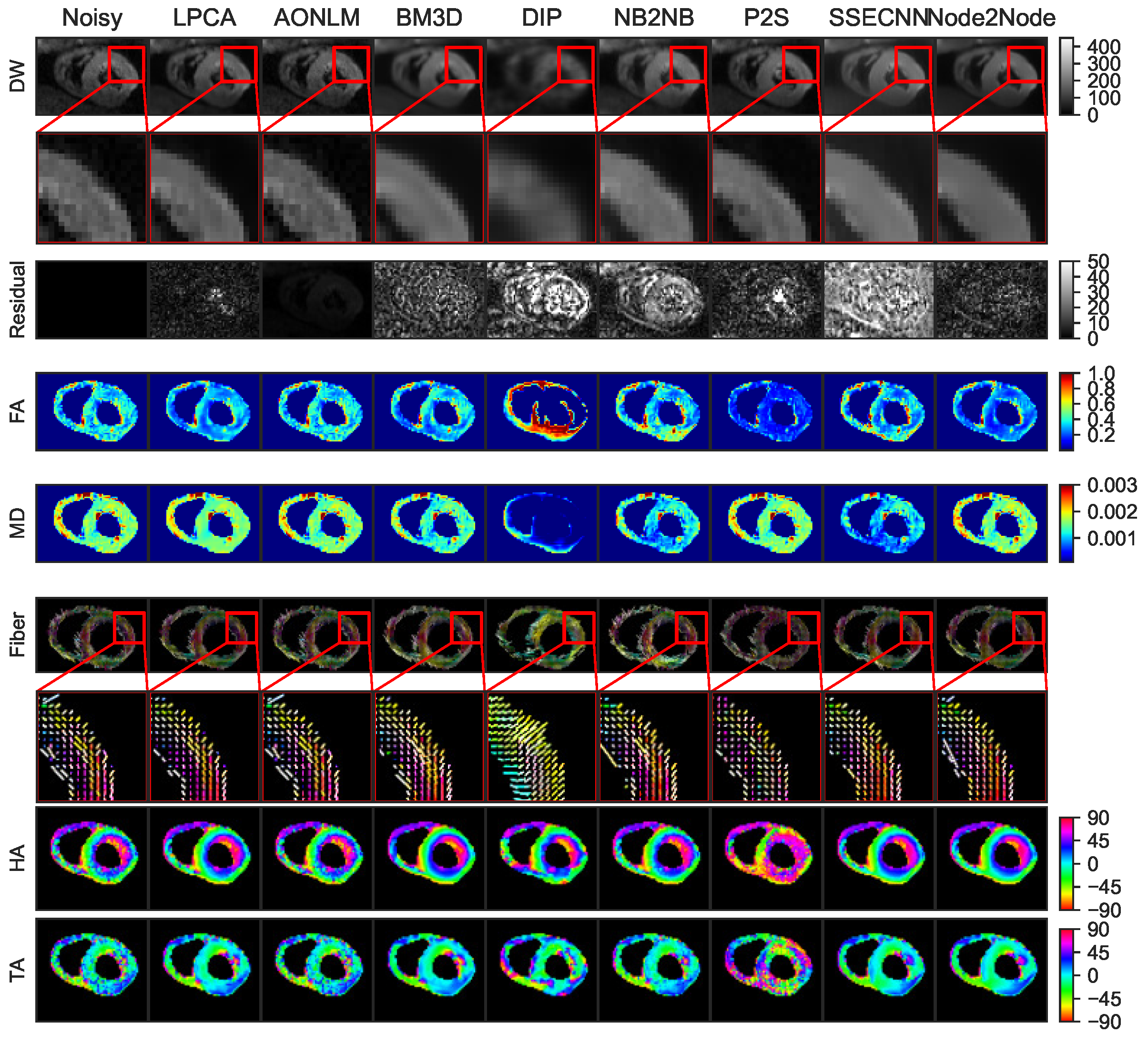
4.2.1. Denoising Results for Ex Vivo Porcine Cardiac DTI

Figure 4 shows the denoising results obtained with different methods on an ex vivo porcine dataset. We observe that the residual values of the DW images generated with BM3D, DIP, NB2NB, and SSECNN are so big that they can not accurately estimate the cardiac fiber orientations or FA and MD maps from the denoised DW images. For instance, the denoised fiber orientations of BM3D and NB2NB are totally disarranged, and the FA values are much higher than those in the noisy ones, while the MD values are much smaller. However, LPCA, AONLM, P2S, and the proposed Node2Node result in small residuals in DW images. In particular, in our proposed model, Node2Node, and LPCA, the residual maps are homogeneous with small values and without structure information. However, the blurring effects of LPCA over Node2Node on FA and MD maps can also be observed. In terms of HA and TA maps, besides BM3D, all the methods can restore the helix and transverse angle distributions, but the TA maps obtained through DIP, NB2NB, and P2S are a little noisy.

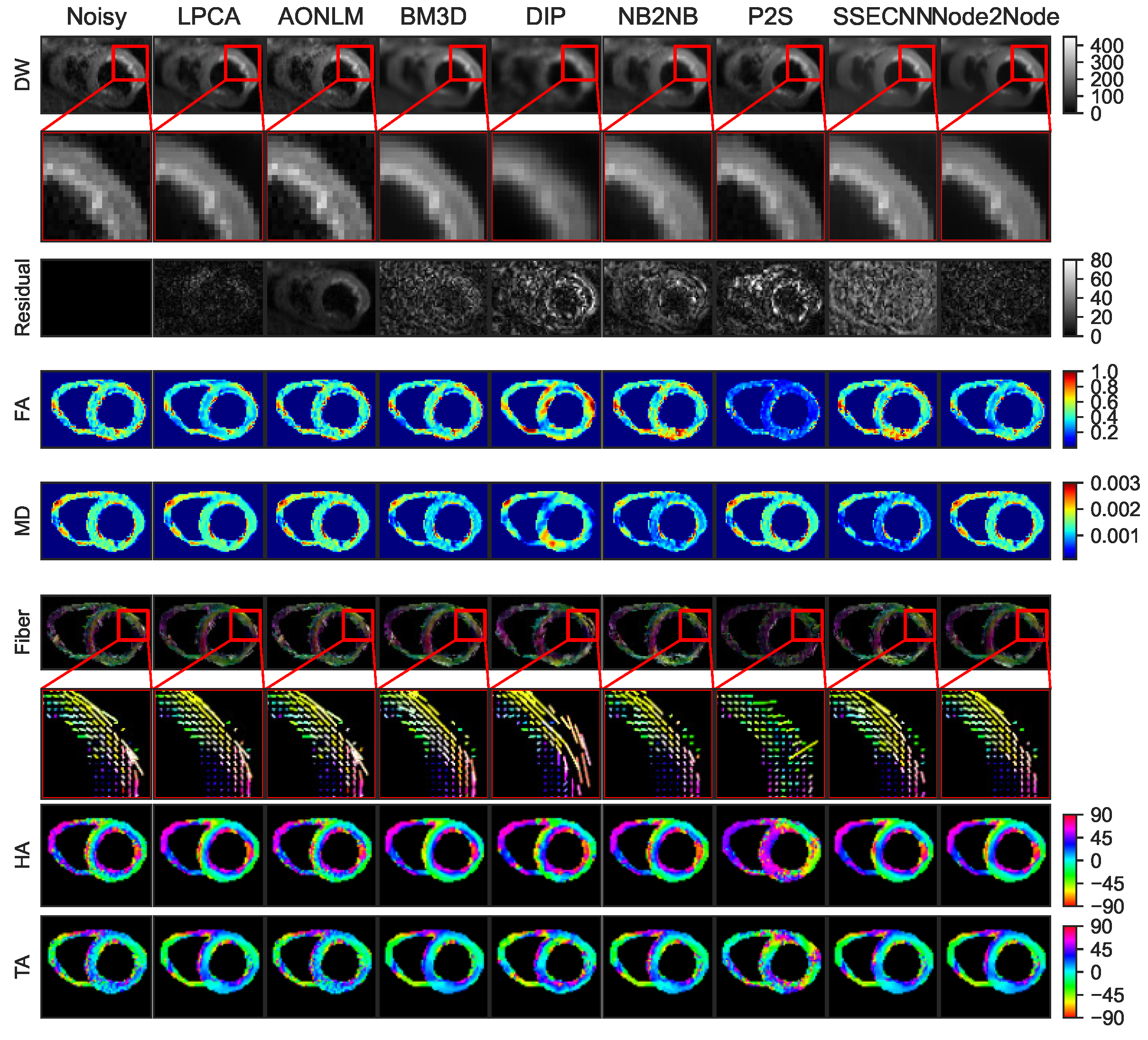
4.2.2. Denoising Results for In Vivo Human Cardiac DTI

In vivo cardiac DTI is more sensitive to noise than other DTI. To further verify the effectiveness of the proposed method, we compare the performance of different methods on removing the noise of in vivo cardiac DTI at different phases. Figure 5 demonstrates the denoising results for cardiac DTI acquired at early systole. We notice that, different from the ex vivo porcine cardiac DTI, the performance of AONLM, Patch2Self, and SSECNN is not good for early-systole cardiac DTI, with the higher residual values and the structural information being contained in the residual maps. In addition, the performance of DIP and NB2NB on in vivo cardiac DTI is much worse, while the performance of BM3D is improved. In terms of FA and MD maps, DIP, NB2NB, P2S, and SSECNN generate more singular FA and MD values; for example, DIP and NB2NB result in FA values close to 1, while P2S leads to FA values close to 0. Regarding the fiber orientations in HA and TA maps, we notice that, after denoising, DIP and P2S can not restore the helical structure of cardiac fibers. Although the other methods can restore the helical structures, AONLM still has some noise remaining. The HA maps obtained using the other methods are comparable, but the TA map obtained using the proposed method is better than the others, with a relatively smooth transition in the transverse angle. The performance of LPCA and BM3D is similar to that of the proposed method, Node2Node, but its TA values at the interaction between the left ventricle and right ventricle are not smooth like those of Node2Node.

Figure 6 illustrates the denoised results for the in vivo cardiac DTI at the end systole phase. We see that the performance of DIP on end systole data is better than that on early systole data. (In the fifth column of Figure 5, the denoised DW image is almost black), but its denoised DW image is still too blurry to tell the myocardium from the background. Like the early systole results, DIP, NB2NB, and SSECNN generate large residual values with obvious structure information remaining (the third row). Although the values in the residual map of the DW images obtained using P2S are not so large, P2S cannot restore the helical fiber architecture (the seventh row). As for AONLM, its denoised result is very similar to the original noisy image; the values of the residual map are very small but with the myocardium structure retained. LPCA, BM3D, and the proposed Node2Node result in lower and random residual values; consequently, their FA, MD, HA, and TA maps are much better than those of the others. In contrast to LPCA and BM3D, the transverse angle derived from the proposed model is smoother than that of LPCA and BM3D.

The denoised results for in the vivo cardiac DTI at the end diastole phase are shown in Figure 7. Different from the results for the systole datasets, the performance of DIP, NB2NB, and SECNN are significantly improved with the residual values of the DW images decreased, but there is still myocardium structure information in their residual maps. Although there are still singular values in their FA and MD maps, DIP can reconstruct the helical myocardium architecture from its denoised DW images. As for P2S, it achieves the worst performance, with extremely low FA values and disarranged fiber orientations. We also find that only LPCA, BM3D, and Node2Node can generate small residual values in the DW images, but the FA values derived from BM3D are little higher, and the TA maps obtained using LPCA and BM3D are worse than those of our method (a little noisy.)

4.2.3. Quantitative Comparisons with SOTA Methods on Real Datasets

The objective assessment metrics for different methods on a real dataset are presented in

Table 2. SNRs and CNRs obtained with different methods for real datasets. The optimal and suboptimal results are highlighted in bold and with underline, respectively.

Method	Porcine Hearts		Early Systole		End Systole		End Diastole
	SNR	CNR	SNR	CNR	SNR	CNR	SNR	CNR
Noisy	0.59	76.20	16.81	137.48	17.38	133.63	16.78	158.94
LPCA	4.71	179.65	43.74	301.06	46.10	314.66	42.50	361.03
AONLM	3.62	168.07	16.77	137.48	17.38	16.31	16.81	158.94
BM3D	1.39	79.79	75.70	469.04	80.56	464.33	77.05	603.10
DIP	0.72	31.83	27.11	195.25	30.90	187.01	32.46	236.86
NB2NB	2.31	59.28	40.58	200.50	42.49	215.58	37.59	241.08
P2S	1.79	120.46	30.12	184.71	32.21	196.76	29.82	220.70
SSECNN	4.34	134.85	48.90	293.19	52.24	278.21	47.12	334.24
Node2Node	6.50	203.58	71.29	477.57	75.60	465.23	67.52	540.70

. It can be seen that for the ex vivo porcine hearts, our method achieves the highest SNR and CNR. Comparing it against the suboptimal method (LPCA), the SNR and CNR are increased by 38% and 13.32%, respectively. However, for the in vivo dataset, BM3D and our method perform much better than the others. BM3D obtains the highest SNR and CNR on the end diastole dataset. However, on both early and end systole datasets, our method generates the best CNR while BM3D achieves the best SNR.

4.3. Ablation Results

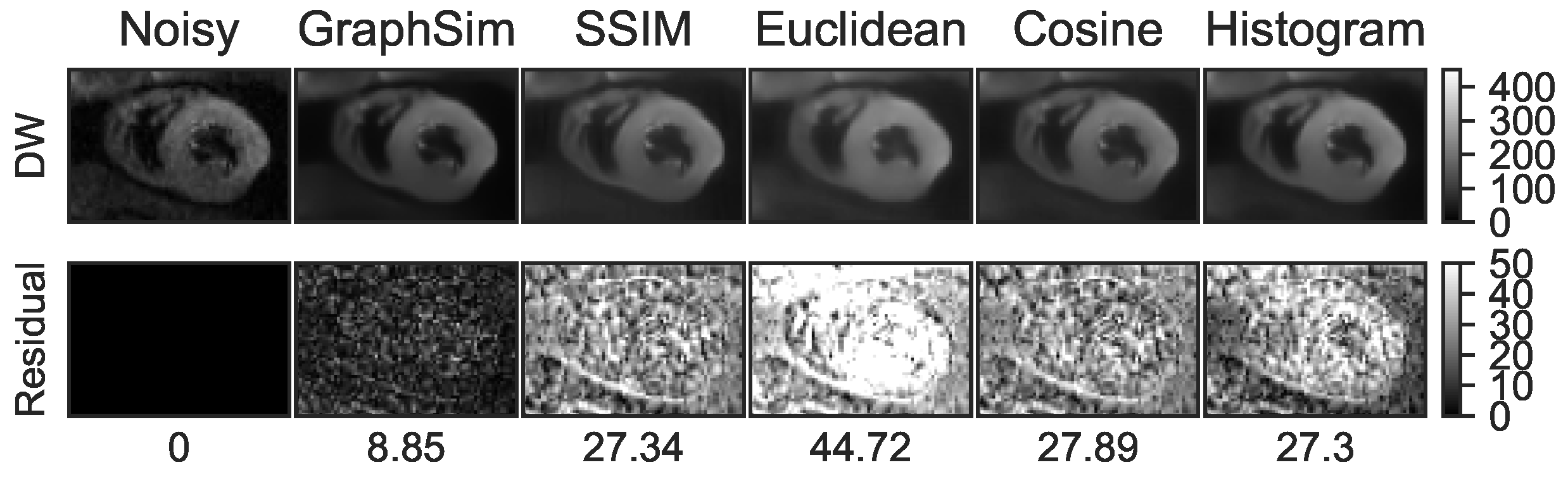
4.3.1. Comparisons in Image Pair Matching Strategies

To validate the superiority of the proposed image pair matching strategy using the similarity of graph framelet transform coefficients (GraphSim), we compare it with four other commonly used similarity measures, including the SSIM used in SSECNN, the Euclidean distance used in NLM and BM3D, and histogram and Cosine similarities. To make a fair comparison, the baseline network structure, the training process, and the optimizing parameters of Node2Node are kept unchanged except its image pair matching strategies. As demonstrated in Figure 8, the proposed image pair matching method results in the smallest random residual maps with a minimum RMSE value of 8.85, which is improved by 67.62%, 80.21%, 68.27%, and 67.58% compared against the SSIM, Euclidean distance, and cosine and histogram similarity measures, respectively. In addition, compared with the other image pair matching methods, the proposed GraphSim can remove the noise without losing the structure information.

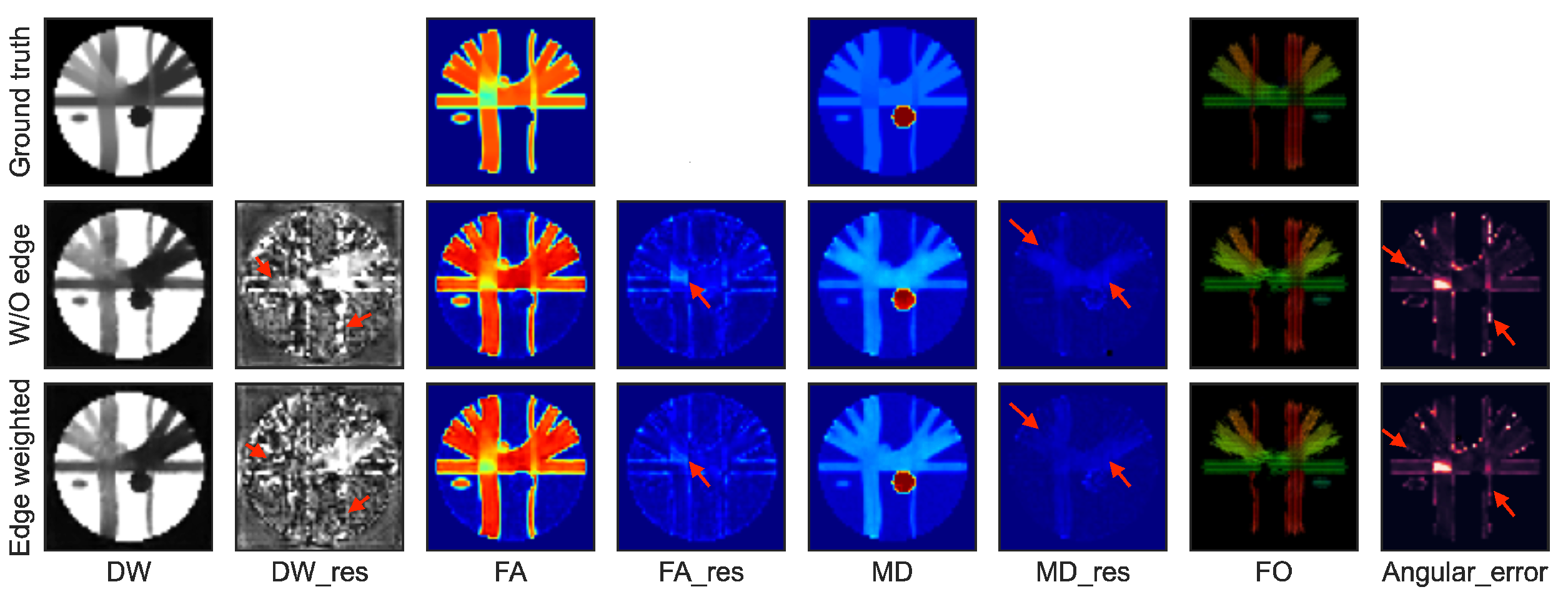
4.3.2. Effects of the Edge-Weighted Loss

To test the effectiveness of the proposed edge-aware loss, and considering that there is a ground-truth for the synthetic dataset, we compare the denoising results of the synthetic dataset with and without edge-aware loss, as illustrated in Figure 9. It can be clearly seen that, with the help of the edge-aware loss, the residual values of the DW images and the FA and MD maps at the edge regions are obviously reduced. Moreover, the angular error between the fiber orientations and the ground-truth at the edge regions is also decreased, as indicated by the red arrows in the Figure 9.

The quantitative comparisons between using (edge-weighted) and not using edge-aware loss (W/O edge) are shown in

Table 3. Quantitative comparisons between using and not using edge-weighted loss.

	Method	RMSE	PSNR	SSIM	AAE
W/O edge	DW images	99.24	33.30	0.97	–
	FA maps	0.033	28.44	0.83	–
	MD maps	3.25 × 10${}^{-5}$	39.68	0.99	–
	Fiber orientations	–	–	–	2.68
Edge-weighted	DW images	86.29	34.51	0.97	–
	FA maps	0.029	29.38	0.85	–
	MD maps	2.95 × 10${}^{-5}$	4 0.52	0.99	–
	Fiber orientations	–	–	–	2.48

. We see that with the edge-aware loss, the RMSE/PSNR of DW images and the FA and MD maps are improved by 13.1%/3.6%, 12.1%/3.3%, and 10.2%/2.1%, respectively. Introducing the edge-ware loss, the SSIMs of the DW images and MD maps do not change, but the SSIM of the FA maps increases from 0.83 to 0.85; in addition, the AAE in fiber orientations is decreased by 7.5%.

5. Discussion and Conclusions

In this work, we propose a novel self-supervised learning-based denoising model, Node2Node, for cardiac DTI datasets. To avoid the influence of noise, it first searches the similar DW image pairs on a graph spectral domain based on the GFT coefficients at different bands, and then uses a ResNet-like architecture to denoise with the searched DW image pairs. Moreover, to avoid the problem of over-smoothing introduced by the denoising, a novel edge-aware loss is presented, which is implemented with the erosion and dilation through the pooling operations, allowing it to adaptively adjust the loss weights on both the edge and smooth regions, therefore promoting the detail-preserving ability of the model. To verify the superiority of Node2Node, we compare it with several state-of-the-art denoising methods, including LPCA, AONLM, BM3D, DIP, Neighbor2Neighbor, Patch2Self, and SSECNN, on a synthetic dataset and two real datasets (ex vivo porcine cardiac DTI and in vivo human cardiac DTI acquired at three different phases). The experimental results demonstrate that the proposed Node2Node can effectively remove the noise in both ex vivo and in vivo cardiac DW images, not influenced by the noise distributions and the number of diffusion directions, allowing it to explore both ex vivo and in vivo myocardial fiber structures with DW images of low SNR.

AONLM, LPCA, and BM3D are the current commonly used methods in clinics to denoise medical images, and AONLM and BM3D fully utilize the self-similarity of image blocks to remove noise. Such of methods require the system to search similar image patches or blocks, which is very time-consuming. In addition, the performance of the patch- or block-similarity-based methods is sensitive to the image quality. For instance, in this work, AONLM performs better on the ex vivo porcine cardiac DTI, while it performs worse on the in vivo human cardiac DTI and the synthetic dataset. This because the noise level in the ex vivo porcine dataset is relatively lower than that in the synthetic dataset, so similar patches can be more accurately found. With the increase in the noise level, the similarity between the image patches is influenced, therefore affecting the denoising performance. In addition, comparing the ex vivo porcine dataset and the in vivo human cardiac dataset, in the former, there are 120 slices, while in the latter, only 1 slice was acquired. This limits the searching space for similar patches in the in vivo data, therefore decreasing the performance of AONLM. Regarding BM3D, it performs much better on the in vivo cardiac DTI than the ex vivo cardiac DTI. The major differences between the ex vivo and in vivo cardiac DTI are the number of diffusion directions and the noise levels. The ex vivo cardiac DTI data were acquired with 30 diffusion directions and a higher noise level (SNR = 0.59), while the in vivo cardiac DTI data were acquired with 12 diffusion directions and a lower noise level (SNR varies from 16 to 18). Since BM3D searches similar blocks and aggregates them along both diffusion directions and volumes, when the number of the diffusion directions is greater, the image blocks along different diffusion directions are the most similar. In this case, aggregating similar blocks along different directions in one DW image along a certain direction may cause problems. This is why BM3D performs worse on the ex vivo cardiac DTI. LPCA can fully exploit the multidirectional redundancy of DW images, and it uses the thresholded principal component decompositions of each 4D local block to remove the noise in DW images. When the number of diffusion directions is not enough, the degree of the redundancy of the local signals is not sufficient; as a result, the performance of LPCA is not good, as expected. This can be observed in the denoising results of the synthetic dataset, where only six diffusion directions are used.

DIP, NB2NB, Patch2Self, and SSECNN are recently proposed unsupervised or self-supervised learning-based image denoising methods. Of these, DIP and Neighbor2Neighbor are used to deal with natural image noise, while Patch2Self and SSECNN are designed for diffusion-weighted images. DIP assumes that the deep network can learn the image priors, meaning that using the random noise as the input and a noisy image as the target, the network can first learn the clean version of the noisy image and then learn the disrupted information. Based on this assumption, DIP uses an early stop strategy to denoise. Even though the DIP can remove the noise and use only one noisy image to train the network, this on-line learning process is not suitable to deal with a series of images since the iteration number of early stop for each individual image may be totally different. It is not practical to denoise DW image volumes by training a DIP network several times. In this work, all the denoised DW images along different diffusion directions are derived with the same early stop setting, which cannot guarantee that all the denoised DW images have already achieved their optimum status; accordingly, it performs worse on all the datasets.

The methodologies of Neighbor2Neighbor and SSECNN are essentially different from that of DIP; they use the self-similarity of different noisy image pairs to denoise rather than the deep network prior. The Neighbor2Neighbor uses a downsampling operation to generate similar image pairs and then uses them to train the denoising network based on the Noise2Noise method, while SSECNN leverages the SSIM between the DW images along different directions to obtain these image pairs. Since the spatial resolution of all the datasets used in this work is not high enough (128 × 128 for the real dataset and 55 × 55 for the synthetic dataset), the image pairs obtained with the nearest-neighbor downsampling may be not similar enough to meet the assumptions of Noise2Noise; therefore, the performance of Neighbor2Neighbor is not satisfactory. SSECNN searches the DW image pairs by maximizing the SSIM between the noisy DW images along different directions. For the synthetic dataset, SSECNN can achieve the better results, while for both ex vivo porcine and in vivo human cardiac DTI datasets, its performance decreases dramatically. This may be caused by the differences in noise distribution among the different datasets. In the synthetic dataset, the noise conforms to the Gaussian distribution, while in the real dataset, the noise usually conforms to the Rician distribution (as illustrated in Figure 10). Rather than using the image pairs to train the network to denoise, Patch2Self uses a linear regression method to denoise. Specifically, for a given voxel along a certain diffusion direction, its clean DW signal is obtained by linearly fitting the DW signals of its surrounding neighbors along the other directions. Since the regression methods are heavily dependent on the amount of data, if the number of diffusion gradient directions or the number of slices is not enough, the bias caused by the linear regression will be significant. That is why Patch2Self performs better on the ex vivo porcine cardiac DTI dataset (30 diffusion directions, 120 slices) but worse on the synthetic (6 directions, 55 slices) and in vivo (12 directions, 1 slice) datasets.

As for the proposed Node2Node model, it achieves almost the best performance on all the datasets, demonstrating its stability and generalization ability. This means it is not sensitive to the noise distribution (it performs well on both the synthetic and real datasets), the number of diffusion directions, or noise levels (no significant difference in performance on the ex vivo and in vivo datasets). In Node2Node, similar DW image pairs are searched based on the GFT coefficients, which allows it to compare the different image pairs on several sub-bands in the spectral domain. Considering that sub-band coefficients of the random noise are relatively slower than those of the signal, accordingly, their contributions on the similarity calculation can be overlooked. Therefore, using GFT coefficients to find the similar image pairs is more robust and stable. This can also be found in the ablation results (Figure 8); the performance of GraphSim used in Node2Node is much better than the others. In addition, as indicated by the red arrows in Figure 9, with the help of edge-aware loss, the denoising performance at the edge regions is clearly improved, demonstrating the effectiveness of the proposed edge-aware loss. However, there are still some limitations in this work. For example, the denoising performance for the regions with fiber crossings (Figure 9) is not good. This may be caused by the few diffusion directions. Additionally, for real data, the model was trained with the ex vivo porcine dataset and directly tested on the in vivo human cardiac dataset without using any transfer learning strategies. Even though the performance on the current in vivo dataset is satisfactory, it will be better to test it on other datasets to further verify the generality of the proposed method.

References

1. Mozaffarian, D.; Benjamin, E.; Go, A.; Arnett, D.; Blaha, M.; Cushman, M.; Das, S.; de Ferranti, S.; Després, J.; Fullerton, H.; et al. Executive Summary: Heart Disease and Stroke Statistics—2016 Update: A Report From the American Heart Association. Circulation 2016, 133, 447. [Google Scholar] [CrossRef] [PubMed]
2. Münzel, T.; Gori, T.; Keaney, J.F., Jr.; Maack, C.; Daiber, A. Pathophysiological role of oxidative stress in systolic and diastolic heart failure and its therapeutic implications. Eur. Heart J. 2015, 36, 2555–2564. [Google Scholar] [CrossRef] [PubMed]
3. Jorge, E.; Amorós-Figueras, G.; García-Sánchez, T.; Bragós, R.; Rosell-Ferrer, J.; Cinca, J. Early detection of acute transmural myocardial ischemia by the phasic systolic-diastolic changes of local tissue electrical impedance. Am. J. Physiol. Heart Circ. Physiol. 2016, 310, H436–H443. [Google Scholar] [CrossRef] [PubMed]
4. Garcia-Canadilla, P.; Cook, A.C.; Mohun, T.J.; Oji, O.; Schlossarek, S.; Carrier, L.; McKenna, W.J.; Moon, J.C.; Captur, G. Myoarchitectural disarray of hypertrophic cardiomyopathy begins pre-birth. J. Anat. 2019, 235, 962–976. [Google Scholar] [CrossRef] [PubMed]
5. Wiest-Daesslé, N.; Prima, S.; Coupé, P.; Morrissey, S.P.; Barillot, C. Non-local means variants for denoising of diffusion-weighted and diffusion tensor MRI. In Proceedings of the International Conference on Medical Image Computing and Computer-Assisted Intervention, Brisbane, Australia, 29 October–2 November 2007; pp. 344–351. [Google Scholar]
6. Coupé, P.; Manjón, J.V.; Robles, M.; Collins, D.L. Adaptive multiresolution non-local means filter for three-dimensional magnetic resonance image denoising. IET Image Process. 2012, 6, 558–568. [Google Scholar] [CrossRef]
7. Lam, F.; Babacan, S.D.; Haldar, J.P.; Weiner, M.W.; Schuff, N.; Liang, Z.P. Denoising diffusion-weighted magnitude MR images using rank and edge constraints. Magn. Reson. Med. 2014, 71, 1272–1284. [Google Scholar] [CrossRef] [PubMed]
8. Lam, F.; Liu, D.; Song, Z.; Schuff, N.; Liang, Z.P. A fast algorithm for denoising magnitude diffusion-weighted images with rank and edge constraints. Magn. Reson. Med. 2016, 75, 433–440. [Google Scholar] [CrossRef] [PubMed]
9. Gramfort, A.; Poupon, C.; Descoteaux, M. Denoising and fast diffusion imaging with physically constrained sparse dictionary learning. Med. Image Anal. 2014, 18, 36–49. [Google Scholar] [CrossRef]
10. Kong, Y.; Li, Y.; Wu, J.; Shu, H. Noise reduction of diffusion tensor images by sparse representation and dictionary learning. Biomed. Eng. Online 2016, 15, 5. [Google Scholar] [CrossRef]
11. Awate, S.P.; Whitaker, R.T. Feature-preserving MRI denoising: A nonparametric empirical Bayes approach. IEEE Trans. Med. Imaging 2007, 26, 1242–1255. [Google Scholar] [CrossRef]
12. Gonzalez, J.E.I.; Thompson, P.M.; Zhao, A.; Tu, Z. Modeling diffusion-weighted MRI as a spatially variant Gaussian mixture: Application to image denoising. Med. Phys. 2011, 38, 4350–4364. [Google Scholar] [CrossRef] [PubMed]
13. Raj, A.; Hess, C.; Mukherjee, P. Spatial HARDI: Improved visualization of complex white matter architecture with Bayesian spatial regularization. NeuroImage 2011, 54, 396–409. [Google Scholar] [CrossRef] [PubMed]
14. Manjón, J.V.; Coupé, P.; Martí-Bonmatí, L.; Collins, D.L.; Robles, M. Adaptive non-local means denoising of MR images with spatially varying noise levels. J. Magn. Reson. Imaging 2010, 31, 192–203. [Google Scholar] [CrossRef] [PubMed]
15. Manjón, J.V.; Coupé, P.; Concha, L.; Buades, A.; Collins, D.L.; Robles, M. Diffusion weighted image denoising using overcomplete local PCA. PLoS ONE 2013, 8, e73021. [Google Scholar] [CrossRef] [PubMed]
16. Fadnavis, S.; Batson, J.; Garyfallidis, E. Patch2Self: Denoising Diffusion MRI with Self Supervised Learning. Adv. Neural Inf. Process. Syst. 2020, 33, 16293–16303. [Google Scholar]
17. Zhang, K.; Zuo, W.; Chen, Y.; Meng, D.; Zhang, L. Beyond a gaussian denoiser: Residual learning of deep cnn for image denoising. IEEE Trans. Image Process. 2017, 26, 3142–3155. [Google Scholar] [CrossRef] [PubMed]
18. Dabov, K.; Foi, A.; Katkovnik, V.; Egiazarian, K. Image denoising by sparse 3-D transform-domain collaborative filtering. IEEE Trans. Image Process. 2007, 16, 2080–2095. [Google Scholar] [CrossRef]
19. Du, Q.; Tang, Y.; Wang, J.; Hou, X.; Wu, Z.; Li, M.; Yang, X.; Zheng, J. X-ray CT image denoising with MINF: A modularized iterative network framework for data from multiple dose levels. Comput. Biol. Med. 2023, 152, 106419. [Google Scholar] [CrossRef]
20. Spuhler, K.; Serrano-Sosa, M.; Cattell, R.; DeLorenzo, C.; Huang, C. Full-count PET recovery from low-count image using a dilated convolutional neural network. Med. Phys. 2020, 47, 4928–4938. [Google Scholar] [CrossRef]
21. Fu, M.; Wang, M.; Wu, Y.; Zhang, N.; Yang, Y.; Wang, H.; Zhou, Y.; Shang, Y.; Wu, F.X.; Zheng, H.; et al. A Two-Branch Neural Network for Short-Axis PET Image Quality Enhancement. IEEE J. Biomed. Health Inform. 2023, 27, 2864–2875. [Google Scholar] [CrossRef]
22. Zhang, J.; Shangguan, Z.; Gong, W.; Cheng, Y. A novel denoising method for low-dose CT images based on transformer and CNN. Comput. Biol. Med. 2023, 163, 107162. [Google Scholar] [CrossRef] [PubMed]
23. Li, Q.; Li, R.; Li, S.; Wang, T.; Cheng, Y.; Zhang, S.; Wu, W.; Zhao, J.; Qiang, Y.; Wang, L. Unpaired low-dose computed tomography image denoising using a progressive cyclical convolutional neural network. Med. Phys. 2023. [CrossRef] [PubMed]
24. Yang, H.; Zhang, S.; Han, X.; Zhao, B.; Ren, Y.; Sheng, Y.; Zhang, X.Y. Denoising of 3D MR images using a voxel-wise hybrid residual MLP-CNN model to improve small lesion diagnostic confidence. In Proceedings of the International Conference on Medical Image Computing and Computer-Assisted Intervention, Singapore, 18–22 September 2022; pp. 292–302. [Google Scholar]
25. Wang, H.; Zheng, R.; Dai, F.; Wang, Q.; Wang, C. High-field mr diffusion-weighted image denoising using a joint denoising convolutional neural network. J. Magn. Reson. Imaging 2019, 50, 1937–1947. [Google Scholar] [CrossRef] [PubMed]
26. Tian, Q.; Bilgic, B.; Fan, Q.; Liao, C.; Ngamsombat, C.; Hu, Y.; Witzel, T.; Setsompop, K.; Polimeni, J.R.; Huang, S.Y. DeepDTI: High-fidelity six-direction diffusion tensor imaging using deep learning. NeuroImage 2020, 219, 117017. [Google Scholar] [CrossRef] [PubMed]
27. Lin, Y.C.; Huang, H.M. Denoising of multi b-value diffusion-weighted MR images using deep image prior. Phys. Med. Biol. 2020, 65, 105003. [Google Scholar] [CrossRef] [PubMed]
28. Tian, Q.; Li, Z.; Fan, Q.; Polimeni, J.R.; Bilgic, B.; Salat, D.H.; Huang, S.Y. SDnDTI: Self-supervised deep learning-based denoising for diffusion tensor MRI. NeuroImage 2022, 253, 119033. [Google Scholar] [CrossRef] [PubMed]
29. Calvarons, A.F. Improved Noise2Noise denoising with limited data. In Proceedings of the IEEE/CVF Conference on Computer Vision and Pattern Recognition, Nashville, TN, USA, 20–25 June 2021; pp. 796–805. [Google Scholar]
30. Huang, T.; Li, S.; Jia, X.; Lu, H.; Liu, J. Neighbor2neighbor: Self-supervised denoising from single noisy images. In Proceedings of the IEEE/CVF Conference on Computer Vision and Pattern Recognition, Nashville, TN, USA, 20–25 June 2021; pp. 14781–14790. [Google Scholar]
31. Krull, A.; Buchholz, T.O.; Jug, F. Noise2void-learning denoising from single noisy images. In Proceedings of the IEEE/CVF Conference on Computer Vision and Pattern Recognition, Long Beach, CA, USA, 15–20 June 2019; pp. 2129–2137. [Google Scholar]
32. Batson, J.; Royer, L. Noise2self: Blind denoising by self-supervision. In Proceedings of the International Conference on Machine Learning, Long Beach, CA, USA, 9–15 June 2019; pp. 524–533. [Google Scholar]
33. Quan, Y.; Chen, M.; Pang, T.; Ji, H. Self2self with dropout: Learning self-supervised denoising from single image. In Proceedings of the IEEE/CVF Conference on Computer Vision and Pattern Recognition, Seattle, WA, USA, 13–19 June 2020; pp. 1890–1898. [Google Scholar]
34. Yuan, N.; Wang, L.; Ye, C.; Deng, Z.; Zhang, J.; Zhu, Y. Self-supervised Structural Similarity-based Convolutional Neural Network for Cardiac Diffusion Tensor Image Denoising. Med. Phys. 2023. [CrossRef] [PubMed]
35. Wang, Y.G.; Zhuang, X. Tight framelets on graphs for multiscale data analysis. In Proceedings of the Wavelets and Sparsity XVIII, San Diego, CA, USA, 13–15 August 2019; Volume 11138, pp. 100–111. [Google Scholar]
36. Garyfallidis, E.; Brett, M.; Amirbekian, B.; Rokem, A.; Van Der Walt, S.; Descoteaux, M.; Nimmo-Smith, I.; Contributors, D. Dipy, a library for the analysis of diffusion MRI data. Front. Neuroinform. 2014, 8, 8. [Google Scholar] [CrossRef]
37. Teh, I.; Burton, R.A.; McClymont, D.; Capel, R.A.; Aston, D.; Kohl, P.; Schneider, J.E. Mapping cardiac microstructure of rabbit heart in different mechanical states by high resolution diffusion tensor imaging: A proof-of-principle study. Prog. Biophys. Mol. Biol. 2016, 121, 85–96. [Google Scholar] [CrossRef]
Figure 1. The overall structure of the Node2Node, consisting of an image pair matching block and a denoising block. Image pair matching is realized by maximizing the similarity between the GFT coefficients of graph nodes, and denoising is implemented with a ResNet-like structure.
Applsci 13 10829 g001
Figure 2. Denoised DW images for the synthetic data and the corresponding residual maps obtained with different methods. The second and fourth rows show the zoomed-in regions to better visualize the details.
Applsci 13 10829 g002
Figure 3. Denoised diffusion metrics for synthetic data obtained with different methods. FA_res and MD_res represent the residual maps of FA and MD, respectively, and AEM indicates the angular error map.
Applsci 13 10829 g003
Figure 4. Denoised results for the ex vivo porcine cardiac DTI dataset obtained with different methods. The 2nd and 7th rows demonstrate the zoomed-in red rectangle regions for DW images and fiber orientations, respectively.
Applsci 13 10829 g004
Figure 5. Denoised results for in vivo human cardiac DTI acquired at early systole phase with different methods. The 2nd and 7th rows demonstrate the zoomed-in red rectangle regions for DW images and fiber orientations, respectively. DIP and P2S achieve the worst performance.
Applsci 13 10829 g005
Figure 6. Denoised results for in vivo human cardiac DTI acquired at end systole phase with different methods. The 2nd and 7th rows demonstrate the zoomed-in red rectangle regions for DW images and fiber orientations, respectively. DIP and P2S achieve the worst performance.
Applsci 13 10829 g006
Figure 7. Denoised results for in vivo human cardiac DTI acquired at end diastole phase with different methods. The 2nd and 7th rows demonstrate the zoomed-in red rectangle regions for DW images and fiber orientations, respectively. P2S achieves the worst performance.
Applsci 13 10829 g007
Figure 8. Comparisons between the different image pair matching strategies. The numbers indicated below the images are the RMSE values of DW images.
Applsci 13 10829 g008
Figure 9. Influence of the edge-aware loss. Red arrows indicate the obvious differences between using (edge-aware) and not using (W/O edge) the edge-ware loss.
Applsci 13 10829 g009
Figure 10. Distributions of noise in real datasets.
Applsci 13 10829 g010