Visual Image Dehazing Using Polarimetric Atmospheric Light Estimation

Abstract

The precision in evaluating global ambient light profoundly impacts the performance of image-dehazing technologies. Many approaches for quantifying atmospheric light intensity suffer from inaccuracies, leading to a decrease in dehazing effectiveness. To address this challenge, we introduce an approach for estimating atmospheric light based on the polarization contrast between the sky and the scene. By employing this method, we enhance the precision of atmospheric light estimation, enabling the more accurate identification of sky regions within the image. We adapt the original dark channel dehazing algorithm using this innovative technique, resulting in the development of a polarization-based dehazing imaging system employed in practical engineering applications. Experimental results reveal a significant enhancement in the accuracy of atmospheric light estimation within the dark channel dehazing algorithm. Consequently, this method enhances the overall perceptual quality of dehazed images. The proposed approach demonstrates a 28 percent improvement in SSIM and a contrast increase of over 20 percent when compared to the previous method. Additionally, the created dehazing system exhibits real-time processing capabilities.

1. Introduction

With the increasing severity of pollution and the gradual deterioration of the environment, haze and smog weather are characterized by a wide-ranging impact and frequent occurrences. In order to protect the environment, the inspection of the environmental quality, especially the sensing and detection of the emission of pollutants, is a problem that must be faced [1,2]. In view of this situation, many countries have set up environmental stations to monitor companies with high pollutant emissions [3]. In haze and smog conditions, the scattering effect causes the attenuation of light transmission intensity and changes in the transmission direction, leading to a reduction in image quality obtained by optical imaging systems. Image degradation makes it difficult to effectively extract and process the information contained therein, causing certain interference in target detection and recognition [4].

Researchers have conducted long-term and in-depth studies on image-dehazing algorithms. Image-dehazing methods are roughly divided into the following two categories: prior-based methods and learning-based methods [5]. Early image-dehazing methods have generally been based on handcraft priors and have produced images with good visibility. With the development of deep learning, in recent years, learning-based methods have dominated image dehazing. He et al. [6] utilized the dark channel prior to obtain the transmission map for dehazing, but their results suffered from color distortion in the sky regions. Benefiting from the universality of the dark channel prior, numerous improved dehazing algorithms based on this prior have been developed subsequently. Deep learning-based methods like Aod-Net [7], MSCNN [8], and PSD [9] face challenges in achieving good universality due to their dependence on the training dataset.

With the advancement of polarized light acquisition technology and polarimetric detectors, polarimetric dehazing algorithms have emerged. Schechner et al. [10,11] were among the first to use rotating polarizers to capture two images of the brightest and darkest regions, estimate polarimetric parameters, and obtain dehazed images. However, these methods lack real-time performance and are not highly applicable to different scenes. Liang et al. [12] utilized the optimized processing of polarimetric angles and degrees to achieve more accurate estimation of polarimetric parameters, resulting in improved dehazing performance. Shen [13] applied regularization constraints to the transmission and dehazed images and achieved noise-free dehazing results through iterative processing, albeit with a longer computation time. Liang [14] regularized polarimetric angles to suppress noise in the dehazed images. Nevertheless, existing polarimetric dehazing algorithms often exhibit subpar performance for distant scenes, prompting the combination of image enhancement or fusion techniques to improve dehazing quality [15,16].

Polarization imaging technology, as a novel electro-optical imaging technique, not only captures the two-dimensional spatial distribution of target light intensity but also obtains the target’s polarization characteristics, including polarization degree, polarization angle, and polarization ellipticity. This complementary information enhances the reconnaissance and identification capabilities of ground targets [17,18]. Moreover, combining polarization imaging technology with traditional airborne imaging detection methods offers unique advantages in highlighting targets, authenticating objects, penetrating smoke and fog, and adapting to various environments, effectively improving the detection capabilities of electro-optical platforms. Consequently, under specific weather conditions, effectively utilizing polarization information improves imaging quality and enhances contrast.

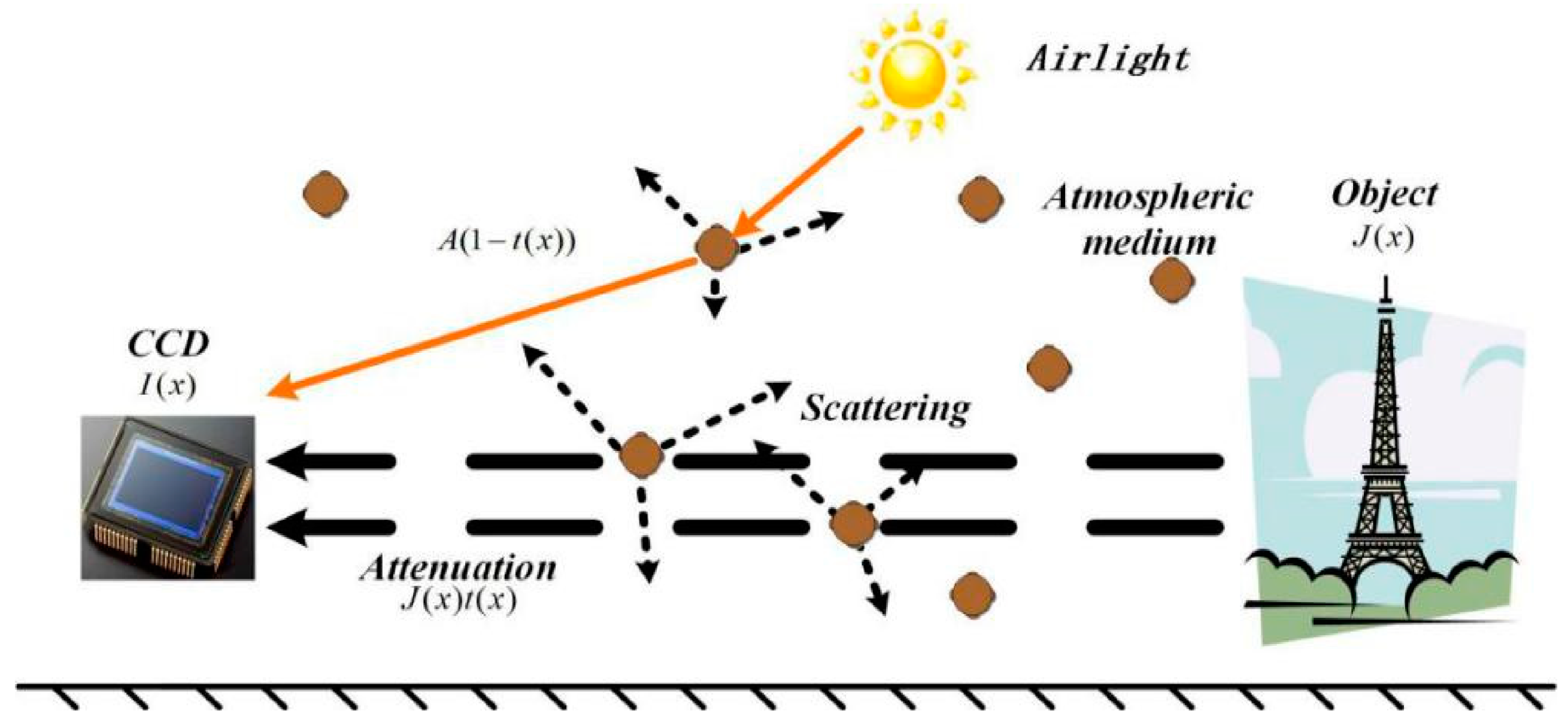
2. Dark Channel Dehazing Theory (DCP)

The dark channel prior dehazing method is based on the atmospheric scattering physical model proposed by McCartney [19] to suppress the impact of scattering effects on the imaging process. The model is illustrated in Figure 1 [20] and is defined as shown in Equation (1).

$$I\left(x\right)=J\left(x\right)t\left(x\right)+A\left(1-t\left(x\right)\right)$$

(1)

In the equation, $I\left(x\right)$ represents the hazy image obtained, x is the spatial coordinate of the pixel, $J\left(x\right)$ is the haze-free image to be restored, A is the global atmospheric light component, and $t\left(x\right)$ denotes the transmission rate. The expression for the transmission rate is defined by Equation (2):

$$t\left(x\right)=e^{-rd\left(x\right)}$$

(2)

In the equation, r represents the atmospheric scattering coefficient, and $d\left(x\right)$ is the light path between field and detector. The dark channel prior principle [6] suggests that in haze-free images, at least one pixel in the non-sky region has an intensity value close to 0. The dark channel of a haze-free image can be represented as follows:

$$J^{dark}\left(x\right)=\underset{y\in \mathsf{\Omega }\left(x\right)}{min}\left(\underset{c\in \{R,G,B\}}{min}{J}^c\left(y\right)\right)$$

(3)

Here, $J^c$ represents each channel of the color image, and $\mathsf{\Omega }\left(x\right)$ denotes a window centered at pixel x. The brightest 0.1% of the pixels’ positions in the dark channel image are recorded, and these recorded pixel positions are mapped back to the hazy image $I\left(x\right)$. Then, the value of the brightest point is considered an estimation of the atmospheric light A. Using the estimated atmospheric light, Equation (1) is normalized as follows:

$$\frac{I^c\left(x\right)}{A^c}=t\left(x\right)\frac{J^c\left(x\right)}{A^c}+1-t\left(x\right)$$

(4)

By simplifying $t\left(x\right)$ as a constant $\tilde{t}\left(x\right)$, we can obtain the following equation by taking the double minimum on both sides of Equation (1):

$$\underset{y\in \mathsf{\Omega }\left(x\right)}{min}\left(\underset{c}{min}\frac{I^c\left(y\right)}{A^c}\right)=\tilde{t}\left(x\right)\underset{y\in \mathsf{\Omega }\left(x\right)}{min}\left(\underset{c}{min}\frac{J^c\left(y\right)}{A^c}\right)+1-\tilde{t}\left(x\right)$$

(5)

The estimated value of the transmission rate $\tilde{t}\left(x\right)$ can be obtained by solving the equation in combination with the dark channel prior principle:

$$\tilde{t}\left(x\right)=1-\underset{y\in \mathsf{\Omega }\left(x\right)}{min}\left(\underset{c}{min}\frac{I^c\left(y\right)}{A^c}\right)$$

(6)

Considering the practical scenario, where particles in the air unavoidably affect the imaging system, to obtain a more natural restored image, we introduce a factor $\omega$ with a value of 0.95 to retain some level of haze. The modified Equation (6) is as follows:

$$\tilde{t}\left(x\right)=1-\omega \underset{y\in \mathsf{\Omega }\left(x\right)}{min}\left(\underset{c}{min}\frac{I^c\left(y\right)}{A^c}\right)$$

(7)

To avoid the restored image from becoming overly white due to very small transmission rate values, we introduce a threshold $t_0=0.1$ for correction. The final restoration formula is as follows:

$$J\left(x\right)=\frac{I\left(x\right)-A}{max(t\left(x\right),t_0)}+A$$

(8)

3. Atmospheric Light Estimation

3.1. Influence of Atmospheric Light Intensity

According to Equations (7) and (8), it is evident that the dehazing effect of the image relies on the accurate estimation of the global atmospheric light A. The intensity of the atmospheric light significantly influences the quality of the dehazed image. While it is challenging to precisely measure the theoretical intensity of the atmospheric light, according to the atmospheric degradation model, we can infer that when the estimated atmospheric light intensity is lower than the theoretical value, the dehazing effect weakens. Conversely, if the estimated atmospheric light intensity is higher than the theoretical value, it can lead to excessive amplification of high-frequency information in the scene or cause some parts of the scene to become too dark or exhibit color abnormalities.

Figure 2 illustrates the impact of the atmospheric light estimation on the dehazing effect. As shown in Figure 2b,c, when we weaken the intensity of A, the dehazing effect is also weakened (green rectangle region). On the other hand, as demonstrated in Figure 2e,f, when we enhance the intensity of A, the dehazing effect becomes more pronounced. However, using an excessively large value for A can lead to the overall darkening of the image, localized dark regions, increased noise, noticeable layering, and overall distortion of the image (red rectangle region).

In He’s method, researchers recorded the coordinates of the brightest 0.1% of points in the dark channel of the hazy image and selected the intensity value of the brightest point at the corresponding position in the hazy image as the estimation for A (atmospheric light). However, this approach has limitations, particularly when the image contains regions with colors similar to the atmospheric light. In such cases, errors in atmospheric light estimation may occur, leading to inaccurate results in transmission rate and restored image. In the next section, we analyze the differences in energy between atmospheric light and scene light polarization. By considering the polarimetric differences, we can separate the global atmospheric light component from the image and use it as a more accurate basis for estimating A. This allows us to overcome the limitations of the previous method and improve the accuracy of the dehazing results.

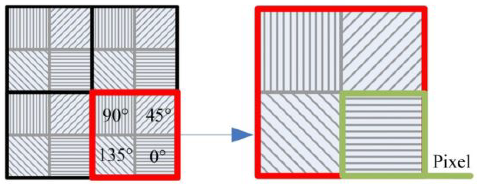
3.2. Polarization State Estimation Model

From the Fresnel reflection law, it is known that objects can produce characteristic polarization determined by their own properties, such as surface morphology, texture, water content, dielectric constant, and incident angle. By exploiting the sensitivity of polarization to physical properties, it is possible to enhance target features and facilitate target identification. A mathematical tool called the Stokes vector [21] S is used to practically and efficiently describe the modification of the polarization states when the light travels and interacts with different materials [22]:

$$S=\left[\begin{array}{c}{s}_0\\ s_1\\ s_2\\ s_3\end{array}\right]=\left[\begin{array}{c}\frac{1}{2}\left(i_0+i_{45}+i_{90}+i_{135}\right)\\ i_0-i_{90}\\ i_{45}-i_{135}\\ i_r-i_l\end{array}\right]$$

(9)

In the Stokes vector representation, $S_0$ represents the intensity element, $S_1$ is the difference between 0° polarization and 90° polarization, $S_2$ is the difference between 45° polarization and 135° polarization, $S_3$ is the difference between right circular polarization and left circular polarization, and i denotes the polarization detection channel. Using the Stokes vector, we can further obtain the polarimetric degree parameter, which characterizes the proportion of the polarization component in the total light intensity:

$$P=\frac{\sqrt{s_1^2+s_2^2+s_3^2}}{s_0}$$

(10)

In our method, we only consider the degree of linear polarization, and therefore, we ignore the $S_3^2$ terms in Equation (10). The degree of linear polarization can be represented by the following formula:

$$P=\frac{\sqrt{s_1^2+s_2^2}}{s_0}$$

(11)

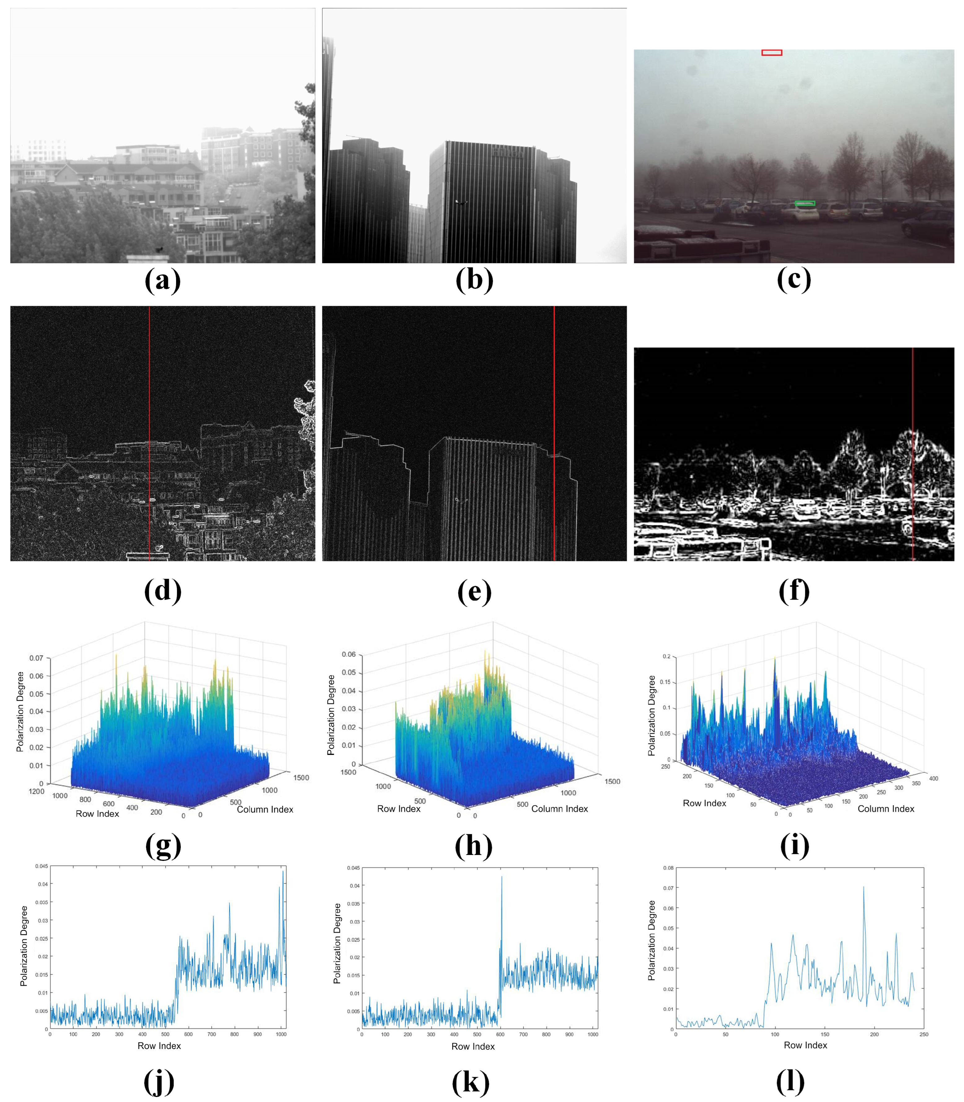
3.3. Polarization Analysis of Natural Scenes

In general, we consider sunlight to be unpolarized light. The polarization information detected by the sensor mainly comes from two sources. One is the polarization phenomenon caused by the scattering of sunlight in the atmosphere, and the other is the polarization phenomenon caused by the reflection of natural objects from the atmospheric light. After conducting polarization analysis and statistical analysis on a large number of polarized images (more than 500), we reached the following conclusions: In general, the polarization degree of atmospheric light is lower than that of natural objects, and this phenomenon is observed in both haze-free and hazy images.

In our analysis and experiments, the polarized images used were obtained from two sources. One part of the data came from the publicly available polarized image dataset, PolarLITIS (https://zenodo.org/record/5547760), accessed on 4 October 2021. The other part of the data was captured using our own polarization detector, which utilizes the Sony IMX250 sensor chip.

In Figure 3, three images with sky regions are displayed. Among them, Figure 3a,b are grayscale images captured by our detector, and Figure 3c is a color image from the PolarLITIS dataset.

It can be observed that the polarimetric degree of the sky region differs significantly from the scene’s polarimetric degree. The polarimetric degree of the sky region is close to 0, while the objects exhibit more pronounced polarization characteristics. In Figure 3c, the part in the green rectangle region is brighter than the part in the red rectangle region but has a lower degree of polarization than what we can see in Figure 3f. In fact, we conducted the above method’s analysis on a large number of natural scene images, and over 85% of the images show this pattern. We measured the sky polarization degree by calculating the ratio of the average polarimetric degree in the sky region to the average polarimetric degree of the entire image.

Figure 4 presents the distribution of this measurement ratio for 517 natural scene images. It can be observed that in over 350 images, the ratio of the sky region’s polarimetric degree to the entire image’s polarimetric degree is less than 10%. Only very few images have a ratio exceeding 30%. In all images, the ratio is less than 1. This indicates that the polarimetric degree of the sky region constitutes a small portion of the overall image polarimetric degree. Such a significant difference allows us to identify the sky region in natural images and use it as the method for estimating the atmospheric light A in the dark channel dehazing algorithm. This enables us to determine a more accurate atmospheric light and enhances the method’s adaptability compared to the original approach.

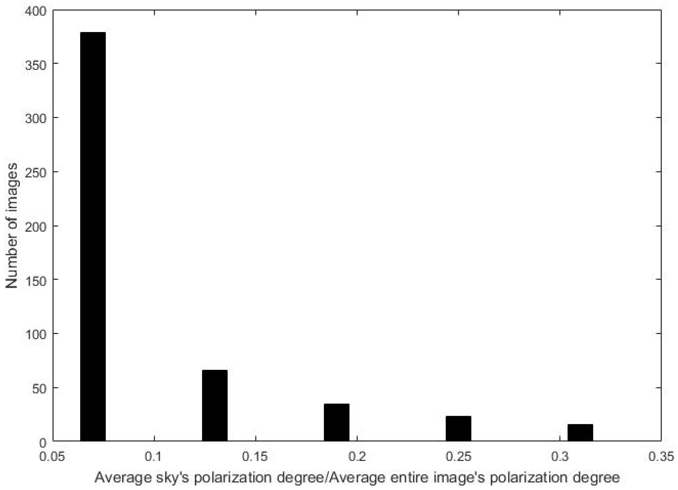
3.4. Polarimetric Degree-Based Atmospheric Light Estimation

Based on the observations mentioned in Section 3.3, we propose a new atmospheric light estimation approach for the dark channel dehazing technique. The prerequisite for using our approach is that we acquire the energy images in four polarization directions, denoted as $i_0,i_{45},i_{90}$, and $i_{135}$, for a natural scene image. The polarimetric degrees for each pixel in the captured image are calculated using Equations (9) and (11).

Next, we search for the lowest 0.1% polarimetric degree pixels in the polarization image and record their positions. From the corresponding positions in the intensity image, we find the brightest pixel to estimate the atmospheric light.

In our practical implementation (introduced in Section 4), due to detector noise, there might be cases of the incorrect computation of sky polarimetric states, leading to errors in the polarimetric degree statistics and automatic identification of erroneous sky regions and atmospheric light estimation. To address these issues, we made certain adjustments to the algorithm. The revised polarimetric degree calculation method is as follows:

$$p^{\prime }\left(x,y\right)=\frac{{\sum }_{\begin{array}{c}i\in {\mathsf{\Omega }}_{xy}\end{array}}{p}_i}{N_{xy}}$$

(12)

In the equation above, $p^{\prime }\left(x,y\right)$ represents the corrected polarimetric degree of pixel $\left(x,y\right)$, ${\mathsf{\Omega }}_{xy}$ is the spatial neighborhood of pixel $\left(x,y\right)$, $p_i$ is the polarimetric degree of pixel in the original polarimetric degree image, and $N_{xy}$ is the number of pixels in ${\mathsf{\Omega }}_{xy}$. The correction in Equation (12) effectively removes polarimetric degree fluctuations caused by noise and bad pixels in the original polarimetric degree image. After this correction, the modified polarimetric degrees may deviate from the true values, but it ensures that no errors are introduced when seeking the region with the minimum polarimetric degree.

Due to the lowest response energy limitation of the polarimetric detector, when the incident light is very low, the pixel grayscale values will be in a very low state, causing the signal intensities of the four polarized angles to be close. As a result, the calculated polarimetric degree will be close to 0, leading to lower polarimetric degrees in non-sky regions compared to the sky regions. If there is a certain region of low signal pixels in the image (with a pixel count exceeding 0.1%), it may lead to errors in estimating the atmospheric light intensity. Therefore, we also make a modification to the atmospheric light estimation approach. We set a threshold $\theta$, and all pixels with polarimetric degrees below this threshold are recorded with their coordinate positions and involved in the subsequent atmospheric light estimation process.

As shown in Section 3.3, in the vast majority of images, the polarimetric degree of atmospheric light is less than 10% of the average polarimetric degree of the entire image. Considering the algorithm’s tolerance, we set the value of $\theta$ to 0.15. Firstly, we calculate the average polarimetric degree of the image, denoted as $p^{\prime }$. Then, we calculate $p_t=\theta \times p^{\prime }$. Next, we record the coordinates of all pixels with a polarimetric degree less than $p_t$. Finally, we select the brightest pixel at the corresponding coordinates in the input image as the estimate of atmospheric light.

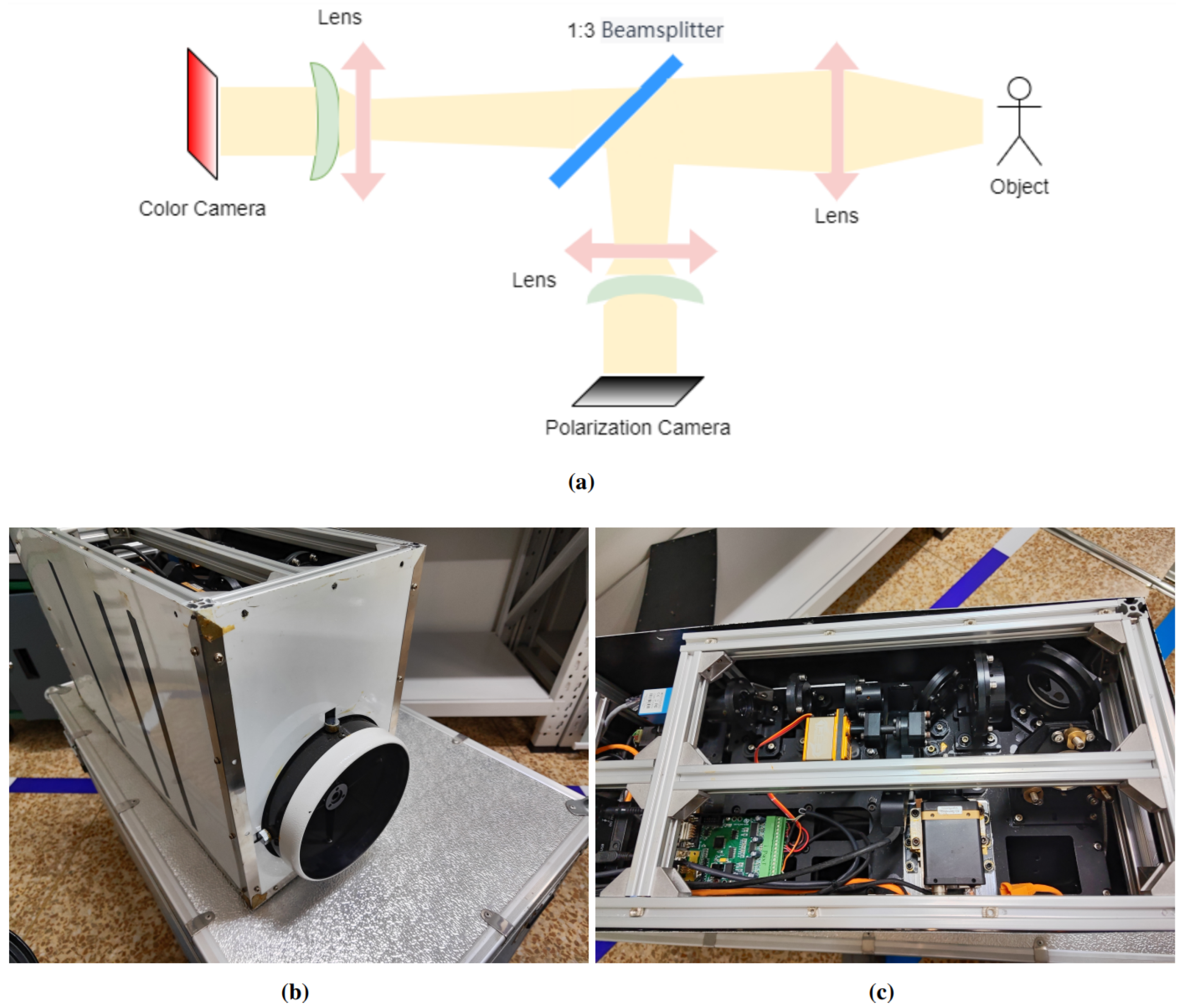
4. Polarimetric Dark Channel Dehazing System

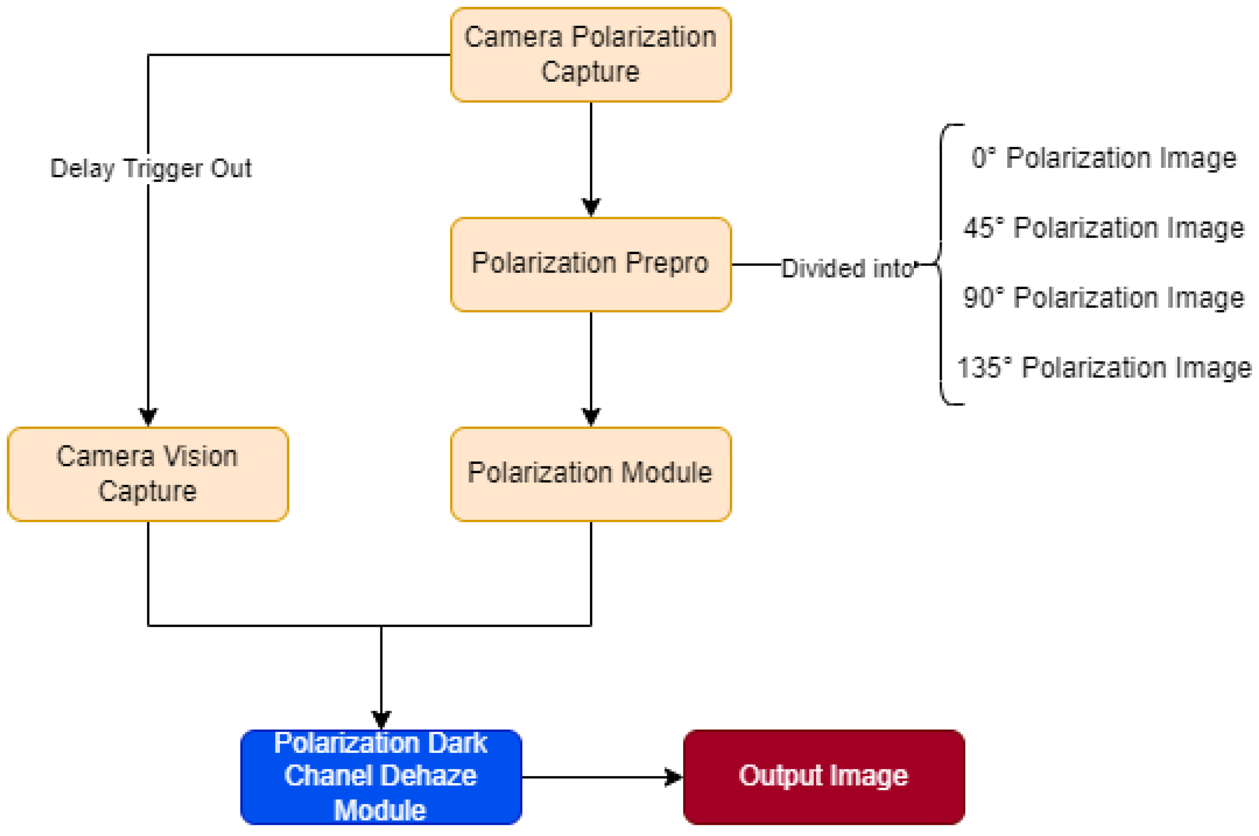
4.1. System Components and Workflow

To achieve the real-time polarization dehazing of scenes, our engineers designed and manufactured a polarization dark channel dehazing system. The equipment we developed is a 150 mm aperture telescope system. Figure 5 shows the optical design and the photographs of the system.

Our system consists of two detectors, including a black-and-white visible light polarization detector and a color visible light imaging detector. The polarization detector uses a CMOS sensor produced by Sony, specifically the IMX250 model. Compared to the imaging detector, this sensor offers higher detection capability and quantum efficiency. As a result, in our optical design, we split the incident light into polarization and imaging detectors in a ratio of 1:3 using a beamsplitter to ensure that the imaging detector receives a higher amount of incident light energy.

To calculate the polarization degree of an image, four intensity images are required for the four polarization directions: 0°, 45°, 90°, and 135°. These four images need to be pixel-level registered. We manufactured the polarization detector using the Sony IMX250 sensor, which is a pixel-level polarization sensor. Each pixel on the chip is equipped with a micro-polarizer in front. The detector has a resolution of 2448 × 2048. Each 2 × 2 pixel group contains polarization information in the four directions. Figure 6 [23] shows the pixel arrangement of this detector. The camera’s characteristics eliminate the need to find a suitable image registration algorithm to achieve pixel-level registration for the four images. In fact, on the IMX250 chip, each group that can be arranged in a $2\times 2$ pattern contains energy from four polarization angles. Therefore, to preserve the original resolution as much as possible, we performed polarization state calculations on each group of four pixels in the $2\times 2$ arrangement. This means that in the polarization state calculation process, each pixel, except for the edge pixels, is reused four times, corresponding to the four pixels in the final map of the degree of polarization (DOP). As a result, the final polarization image has a resolution of $2447\times 2047$.

Our color visible light camera has a resolution of $2048\times 2048$ pixels. To achieve pixel-level alignment with the polarization camera, we used the ROI (region of interest) mode of the polarization camera for image acquisition. We set the ROI image center to be the center of the target surface and output images with the actual resolution of the color visible light camera. Through optical design, we ensured that the center pixels of both cameras overlap, thus obtaining images with the same field of view and resolution.

Figure 7 shows the system workflow. During operation, the polarization detector is responsible for capturing polarization images and providing them to the polarization calculation module to generate polarization degree images. The acquisition detector receives a delayed trigger signal from the polarization detector, then exposes and captures color images. Subsequently, the polarization degree images and color images are passed to the dark channel dehazing module for haze removal processing. The final output is a color dehazed image.

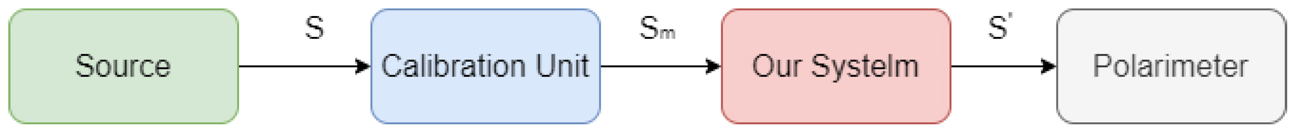
4.2. Polarization Calibration

Due to the incomplete polarization-preserving characteristics of the imaging system, the polarization state of the incident light will change after being transmitted through the imaging system. Therefore, the polarization state calculated from the polarization images is not the same as the polarization state of the incident light. To address this issue, polarization calibration is necessary to accurately calibrate the polarization characteristics of the imaging system. This involves measuring and characterizing the system’s polarization response using known polarized light sources and using the calibration data to correct the detected polarization images. By performing polarization calibration, we can obtain more accurate polarization information and ensure the reliability of the polarization-based imaging system.

The effect of the transmission medium on the polarization state of light can be represented by the Mueller matrix M. For the incident light with polarization state S, after passing through the telescope imaging, the polarization state becomes $S^{\prime }$, and it can be expressed as

$$S^{\prime }=M\times S$$

(13)

where M is the Mueller matrix of the imaging system, representing the deviation of polarization information introduced by the imaging system itself. From Equation (13), we can see that the polarization state we collected is the polarization state changed by the system from the original polarization state, resulting in a deviation from the true polarization information of the incident light. To obtain the incident light’s S, we need to calculate the Mueller matrix M through calibration and then use Equation (14) to solve for the incident light’s S:

$$S=M^{-1}\times S^{\prime }$$

(14)

We used the four-point calibration algorithm to calibrate the system. As indicated by Equation (13), to calculate the Mueller matrix M of the system, we need a known polarization state of the incident light. Therefore, we placed a linear polarizer between the light source and the system to modulate the incident light S, obtaining the known Stokes vector $S_m$. The energy then passes through our imaging system and reaches the polarized detector, resulting in the measured Stokes vector $S^{\prime }$. The calibration setup is illustrated in Figure 8. The calibration unit in the figure represents the linear polarizer used to modulate the incident light S and obtain the known polarization state light source $S_m$. By changing the rotation angle of the linear polarizer, we can acquire various known polarization states. Next, utilizing Equation (15), we can solve for the system’s Mueller matrix M:

$$\begin{array}{c}\hfill S^{\prime }=M\times S_m\\ \hfill M=S^{\prime }\times S_m^{-1}\end{array}$$

(15)

We modulate the incident light four times by adjusting the angle of the linear polarizer to obtain the known polarization states $S_{m1}$, $S_{m2}$, $S_{m3}$, and $S_{m4}$ as the calibration light sources. Next, we use the polarization camera to capture four images, resulting in the measured polarization states $S_1^{\prime }$, $S_2^{\prime }$, $S_3^{\prime }$, and $S_4^{\prime }$ after passing through the telescope system. We can solve for the system’s Mueller matrix M, as shown in Equation (16):

$$M=\left[\begin{array}{cccc}{S}_1^{\prime }& S_2^{\prime }& S_3^{\prime }& S_4^{\prime }\end{array}\right]{\left[\begin{array}{cccc}{S}_{m1}& S_{m2}& S_{m3}& S_{m4}\end{array}\right]}^{-1}$$

(16)

The Mueller matrix of the polarizer is

$$M_p=\frac{1}{2}\left[\begin{array}{cccc}{M}_{p11}& M_{p12}& M_{p13}& 0\\ M_{p21}& M_{p22}& M_{p23}& 0\\ M_{p31}& M_{p32}& M_{p33}& 0\\ 0& 0& 0& M_{p44}\end{array}\right]$$

(17)

The elements in the matrix above are defined as follows:

• $M_{p11}=g_1+g_2$
• $M_{p12}=M_{p21}=\left(g_1-g_2\right)cos2\theta$
• $M_{p13}=M_{p31}=\left(g_1-g_2\right)sin2\theta$
• $M_{p22}={\left(\sqrt{g_1}-\sqrt{g_2}\right)}^2{cos}^{2}2\theta +2\sqrt{g_1{g}_2}$
• $M_{p23}=M_{p32}={\left(\sqrt{g_1}-\sqrt{g_2}\right)}^{2}cos2\theta sin2\theta$
• $M_{p33}={\left(\sqrt{g_1}-\sqrt{g_2}\right)}^2{sin}^{2}2\theta +2\sqrt{g_1{g}_2}$
• $M_{p44}=2\sqrt{g_1{g}_2}$

In the equations above, $g_1$ and $g_2$ represent the transmittance of the polarizers in their polarization direction and perpendicular direction, respectively. For ideal polarizers, $g_1=1$ and $g_2=0$. $\theta$ is the angle between the polarization axis of the polarizer and the X-axis of the coordinate system.

5. Results and Discussion

In this section, we conduct experiments on natural scenes using our system and method for haze removal. To validate the effectiveness of our approach, we compare it with the original dark channel prior-based haze removal method. We discuss the advantages of our method in terms of image quality, accuracy of atmospheric light estimation, and adaptability to different scenes. Finally, we point out the limitations of our method, providing support for future research.

5.1. Experimental Environment

As in Section 3.3, the experimental results presented in the following images are sourced from two parts. One part is from the polarization dark channel dehazing system introduced in Section 4, and the other part is from the polarization image dataset PolarLITIS (https://zenodo.org/record/5547760 accessed on 1 August 2023).

Our experimental system consists of two components. One part is the image acquisition system described in Section 4, and the other part is the data-processing system. This system is operated by a computer with an Intel(R) Core(TM) i7-9700 CPU running at 3.00 GHz, a NVIDIA GeForce RTX 3060 graphics card, and 32 GB RAM. The algorithm implementation is based on the Python programming language.

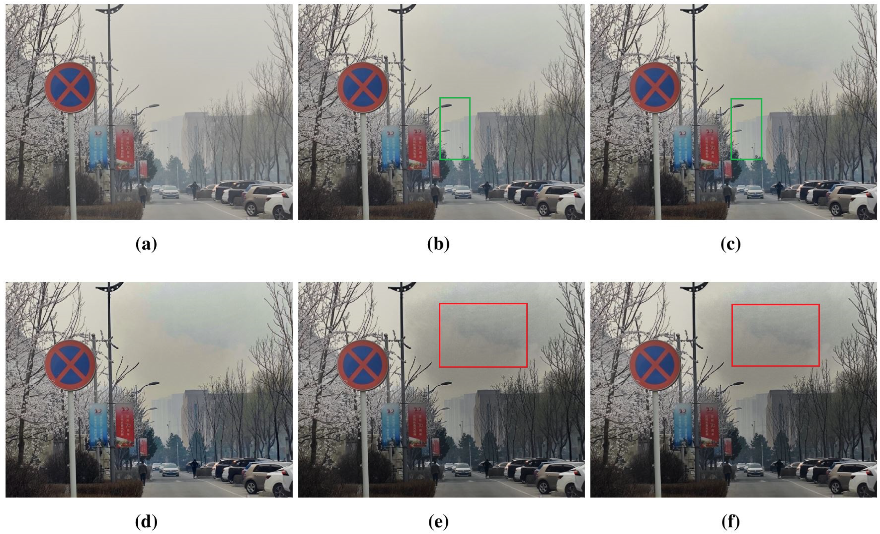
5.2. Experimental Results

Figure 9 represents the intensity images of four polarization angles and polarized degree images acquired using the polarization camera. From Figure 9f, it can be observed that the polarization degree is quite low in the sky region. Among them, the portion highlighted by the green rectangle exhibits the lowest polarization degree. According to the proposed method, the intensity value of this region in the original image is used as an estimate for the atmospheric light.

Figure 10 presents the actual captured and dehazed results using our system. It can be observed that when the haze is relatively bright, the classical dark channel prior dehazing method (Figure 10b) exhibits estimation bias in atmospheric light A. It considers the brightness of the red rectangle region in Figure 10a as the estimate for atmospheric light. This region corresponds to a white traffic sign on the ground, and its value in dark channel map shown in Figure 10d is higher than that of the sky region. In reality, this region has the highest brightness values in both the dark channel image and the original image.

In Figure 9f, the red rectangle region represents the location of the highest pixel value in the dark channel map of the foggy image shown in Figure 10a. However, in the polarimetric image, the corresponding pixel has a high polarimetric value. By using our atmospheric light estimation method, the intensity value at this position would not be selected as an option for the atmospheric light value. On the other hand, the green rectangle region has the lowest polarimetric value, and its intensity value in the original foggy image Figure 10a is chosen as our final estimate for the atmospheric light intensity. In Figure 10a, the average dark channel value within the red rectangle region is 253, which is close to saturation, while the dark channel value within the region marked with a red rectangle is 132. It is evident that the estimation method for atmospheric light in the original dark channel prior algorithm has overestimated the intensity value of the atmospheric light. In Section 3.1, we conduct an analysis of the influence of the atmospheric light intensity on the dehazing algorithm. It is observed that an overestimation of the atmospheric light intensity can lead to a darkening of the overall image, localized darkening regions, increased noise, prominent layering, and overall distortion in the image.

Figure 10b shows the result of the original dark channel prior to the dehazing method. It can be observed that compared to the original image, this image has a significant reduction in brightness, overall lower brightness, and substantial color distortion in the blue sky region. Figure 10c displays the result after using the proposed approach. It preserves the original image’s brightness while ensuring effective dehazing. The color restoration of the sky region is notably improved.

Figure 10e,f illustrate the dark channel map and transmission maps estimated by the original dark channel prior method and the proposed method. As indicated by Equation (7), due to the overestimation of atmospheric light by the DCP method, the estimated transmission rate of the image becomes higher. Moreover, as stated in Equation (8), higher transmission rates result in overall darkening and color shifts in the dehazed image. By employing the proposed method for re-estimating atmospheric light, the transmission rate of the image is reduced, leading to a more natural brightness and color in the dehazed image.

The green rectangular sections in Figure 10b,c are expanded in Figure 11a,b. Due to the original DCP algorithm’s overestimation of the ambient light intensity, the color of the building looks darker in Figure 11a, and the intensity of the red component in RGB diminishes. As a result, the restored red color is hardly visible, and the contrast between the windows and the structure is minimal, making it difficult to discern their borders. Because of the improved color restoration effect, the contrast between the building and the windows is larger in Figure 11b, and their borders are clearly discernible. Our approach keeps a better blue component in the sky region, resulting in a more natural and realistic sky background. In comparison, the original DCP approach produces a darker sky area with a slightly buried blue component.

We use the PSNR (peak signal-to-noise ratio) and SSIM (structural similarity index) [24] to objectively evaluate the quality of the dehazed images. The PSNR of Figure 10b is 13.0365, with an SSIM of 0.8024, while Figure 10c has a PSNR of 16.2242 and an SSIM of 0.8987. A higher PSNR indicates better image quality after processing compared to the original image, while a larger SSIM indicates greater structural similarity between the processed and original images. It can be observed that our method, when compared to the original DCP algorithm, preserves the structural integrity of the original image better and achieves higher image quality.

To provide a clearer and more intuitive demonstration of the effectiveness of our proposed method, Figure 12 showcases the results in a concatenated manner. At the boundary between the building and the sky region, there is a certain amount of halo and stratification (particularly prominent in the red rectangle region), which overall creates an unpleasant visual experience.

In fact, our method remains effective in handling images taken during rainy and smoggy weather conditions. Figure 13 demonstrates the dehazing effect on images captured under rainy and smoggy weather. The proposed method exhibits favorable performance in terms of clarity and color restoration.

To objectively evaluate the effectiveness of our method, we selected haze-free images from the publicly available dataset PolarLITIS. We then applied a fogging process to obtain the foggy versions of these images. Subsequently, we used both the original dark channel prior (DCP) method and our proposed method to perform haze removal on these foggy images. Finally, we utilized the SSIM to quantify the similarity between the dehazed images and the haze-free images in the dataset. A higher SSIM value indicates that the dehazed image is closer to the original haze-free image, which also signifies better dehazing results. Figure 14 presents the experimental results. Subjectively, compared to the original DCP method, the proposed method shows greater similarity to the real haze-free image in terms of color and brightness. Objectively, the SSIM value between the original DCP result and the original haze-free image is 0.7235, while the SSIM value between the proposed method’s result and the original haze-free image is 0.9276. This indicates that the proposed method better restores the real scene.

We applied both the original DCP method and the proposed method to 95 artificially hazy natural scene images. We evaluated the SSIM between their respective dehazed results and the real haze-free scene images. Figure 15 presents the results of the SSIM evaluation. Overall, the proposed method demonstrates higher average SSIM and lower variance compared to the original DCP method. This suggests that, in most cases, the proposed method offers better image restoration performance and higher stability. In this experiment, we intentionally selected more images where the original DCP method inaccurately estimated the atmospheric light intensity to highlight the advantage of the proposed method in dehazing such images.

We evaluated the proposed method using the image sub region’s contrast.

Table 1. Contrast comparison results.

Image	Hazy Image	DCP	Proposed
Figure 10a	0.1918	0.2605	0.3486
Figure 13a	0.0853	0.1959	0.2515
Figure 13b	0.0391	0.0811	0.0791
Figure 14b	0.1683	0.3006	0.3154

presents the contrast evaluation results for the regions marked with yellow rectangles in Figure 10, Figure 13 and Figure 14. The bold numbers in the table represent the maximum contrast values for each image under different algorithms.

It can be observed that both the original DCP and the proposed method effectively enhance the contrast of the hazy images. However, the proposed method exhibits greater stability, with an overall higher enhancement compared to the original DCP, which results in a 28% improvement in SSIM and an increase in contrast of more than 20% when compared to the original DCP.

We contrasted the proposed approach with two traditional dehazing approaches put forth by Tran [25] and Fattal [26] as well as two more recent approaches, RTVP [15] and GLPF [12]. The dehazing outcomes of several algorithms under cloudy, polluted, and wet weathers are shown in Figure 16.

In Figure 16, although DCP has a good capacity to restore the visual quality, it occasionally causes color changes or excessive darkness in the images and more visible halos around object edges. For instance, scene 1 has color changes, while all scenes have an overly dark picture. This problem is caused by the algorithm overestimating the atmospheric light as described in Section 3.1. Images dehazed using Tran’s approach have stronger contrast, but the colors of the result are often over-saturated since his algorithm is not physically based and may underestimate the transmission. The statistical methodology used by Fattal requires enough color information and variance. If the haze is intense, his method cannot effectively estimate the transmission because the color is faint and the variance is too low, resulting in a dehazed image with localized darkening and jarring color transitions. RTVP uses scene polarization to compute the target energy prior to air transmission. This causes an overestimation of the target energy in picture regions with low polarization, resulting in overexposure in these areas. This effect is especially noticeable in the sky areas of Scenes 1 and 2. GLPF can improve the preservation of scene brightness, bringing it closer to the actual ambient light. However, its dehazing impact is weak, resulting in low visual contrast. Our proposed solution keeps the brightness of the image while providing a more prominent dehazing impact. Our approach exhibits good ambient light intensity and contrast in all scenes. It also does a good job at dehazing distant objects in hazy environments.

As objective assessment measures for the dehazing methods, we employed image entropy, local contrast (calculated from the green rectangular region in Figure 16), and SSIM. Image entropy describes the quantity of information in the image, local contrast describes the algorithm’s capacity to improve the distinguishability of object edges, and SSIM quantifies the retention of structural information in images before and after dehazing.

Table 2. Evaluations of algorithms.

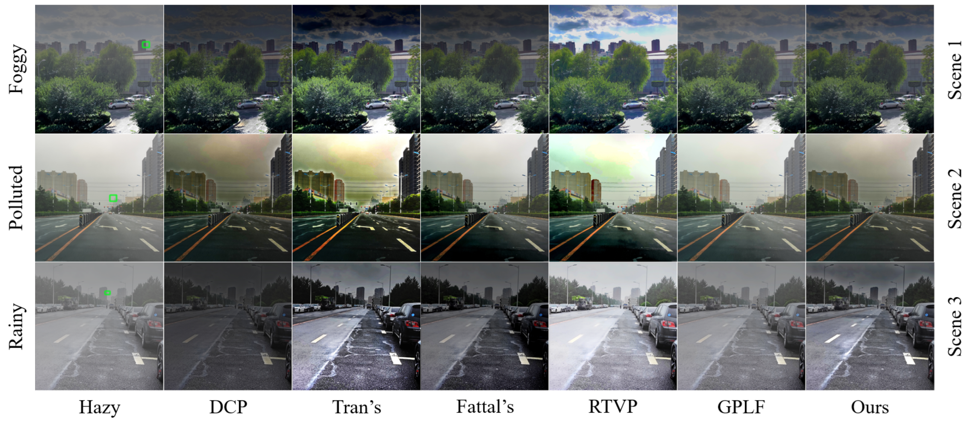
Scene	Evaluation Method	Hazy	DCP	Tran’s	Fattal’s	RTVP	GLPF	Proposed
	Entropy	7.2522	7.7512	7.8001	7.8011	7.8472	7.7801	7.9495
Scene 1	Contrast	0.1918	0.2605	0.3704	0.3401	0.7401	0.2751	0.3486
	SSIM	-	0.8024	0.7725	0.8137	0.7714	0.8554	0.8987
	Entropy	6.8675	7.6453	7.8739	7.8429	7.8781	7.2325	7.8885
Scene 2	Contrast	0.0391	0.0811	0.0947	0.0651	0.0798	0.0464	0.0791
	SSIM	-	0.6716	0.6357	0.7145	0.6681	0.8052	0.7768
	Entropy	7.8913	7.9469	7.8739	7.9478	7.9485	7.9256	7.9509
Scene 3	Contrast	0.0853	0.1959	0.2654	0.2135	0.1978	0.1214	0.2515
	SSIM	-	0.6161	0.6362	0.6478	0.6604	0.8151	0.7998

displays the evaluation results for each subfigure in Figure 16.

For each measure, we use bold type to indicate the highest value and underlining to represent the second-highest value in Table 2. It can be observed that our approach obtains the maximum entropy value across all scenes. RTVP has very high contrast in Scene 1; however, this is due to overexposure in the sky area. Tran’s approach provides the strongest contrast in Scenes 2 and 3, which is related to its extreme color distortion. The approach we propose preserves acceptable brightness and color accuracy while maintaining a high level of contrast. In terms of structural similarity, GLPF performs best because its dehazing impact is less significant, resulting in structural similarity that is closest to the original picture. However, our approach preserves the structure of the original image while producing a good dehazing effect.

5.3. Limitations of the Proposed Method

In the evaluation results shown in Figure 15, although the proposed method demonstrates a clear advantage, there are instances where its performance is lower than or similar to the original DCP method. These cases typically involve images without sky regions or containing very dark elements. In images without sky regions, the physical significance of using low polarization values to determine atmospheric light is weakened. While our method can still probabilistically determine the atmospheric light region correctly in such images since in areas with heavier fog, their polarization is often lower, this is not a high-probability event. In images with very dark elements, the intensity across the four polarization angles becomes similar, resulting in lower polarization values in these areas. However, these darker regions actually imply lower fog concentration, and estimating them as atmospheric light regions would lead to poor dehazing results. Both scenarios introduce uncertainty into our method’s polarization calculation, causing potential inaccuracies in estimating the atmospheric light region.

Figure 17 shows an intentionally collected image that lacks a sky region and contains very dark elements. The green rectangle in Figure 17a represents the atmospheric light location estimated by the proposed method, while the red rectangle represents the atmospheric light location estimated by the original DCP method. For extremely dark regions, our polarization detector’s energy values at the four angles are similar, resulting in a low calculated degree of polarization. Consequently, this region is selected as the atmospheric light estimation region by our approach. However, it is evident that this region is not a reasonable atmospheric light estimation region. Ultimately, due to the underestimated atmospheric light estimation, the image-dehazing effect is weakened.

6. Conclusions and Future Work

6.1. Achievements and Contributions

The main achievements and contributions of our work include the following:

(1) This paper proposes a method for estimating atmospheric light intensity using scene polarization state and applying it to the dark channel prior method to achieve haze removal in hazy images.

(2) To achieve real-time haze removal, an imaging and processing system for hazy scenes is designed and fabricated. The cameras in the system capture frames at a maximum rate of 50 Hz. We used CUDA programming on the NVIDIA GTX 3060 GPU to achieve a single-frame picture dehazing processing time of less than 5 ms, which is far faster than the 20 ms image capture time. This signifies that the system is capable of real-time image-dehazing processing.

(3) We performed an analysis of the natural scene’s polarization characteristics and the influences of atmosphere estimation in the dehazing method, which is introduced in Section 3.3.

(4) The effectiveness of the proposed method was validated on both publicly available datasets and real-world collected data. The method’s performance was analyzed through subjective perception and objective evaluation techniques. The results demonstrate that the proposed method outperforms the original DCP in terms of haze removal, particularly in hazy images containing sky regions. Compared to the original DCP, the proposed approach showed a 28% improvement in SSIM and an increase of over 20% in contrast. The results demonstrate that the proposed method outperforms the original DCP in terms of haze removal, particularly in hazy images containing sky regions.

6.2. Future Work

As discussed in Section 5.3, the proposed method might not perform as well on images that lack sky regions or contain darker elements. Therefore, we plan to make improvements specifically for such images. The improvements will include, but are not limited to, refining the estimation of atmospheric light by considering not only low polarization values as the sole criterion but also leveraging certain characteristics of the scene’s dark channel image for a more accurate estimation. In addition, we will investigate how linear polarization information from other frequent characteristics, such as strongly polarized surfaces, may be used to estimate atmospheric light A.

Dehazing the sky region is required because fog might cause color changes in this region. However, when processing specific images, our approach may occasionally yield unrealistic dehazing effects in the sky region as shown Figure 10c. We relate this phenomenon to our direct use of the brightness from the sky region with the lowest polarization as an estimate of the atmospheric light intensity, which may have resulted in an increased dehazing impact in the sky region, according to our study. As a result, we will examine specific approaches to dealing with the sky region to ensure that the outcomes are more realistic.

References

- Xie, C.; Nishizawa, T.; Sugimoto, N.; Matsui, I.; Wang, Z. Characteristics of aerosol optical properties in pollution and Asian dust episodes over Beijing, China. Appl. Opt. 2008, 47, 4945–4951. [Google Scholar] [CrossRef] [PubMed]
- Edner, H.; Ragnarson, P.; Spännare, S.; Svanberg, S. Differential optical absorption spectroscopy (DOAS) system for urban atmospheric pollution monitoring. Appl. Opt. 1993, 32, 327–333. [Google Scholar] [CrossRef] [PubMed]
- Xu, F.; Lv, Z.; Lou, X.; Zhang, Y.; Zhang, Z. Nitrogen dioxide monitoring using a blue LED. Appl. Opt. 2008, 47, 5337–5340. [Google Scholar] [CrossRef] [PubMed]
- Yi, W.; Liu, H.; Wang, P.; Fu, M.; Tan, J.; Li, X. Reconstruction of target image from inhomogeneous degradations through backscattering medium images using self-calibration. Opt. Express 2017, 25, 7392–7401. [Google Scholar] [CrossRef] [PubMed]
- Yang, G.; Yang, H.; Yu, S.; Wang, J.; Nie, Z. A Multi-Scale Dehazing Network with Dark Channel Priors. Sensors 2023, 23, 5980. [Google Scholar] [CrossRef] [PubMed]
- He, K.; Sun, J.; Tang, X. Single image haze removal using dark channel prior. IEEE Trans. Pattern Anal. Mach. Intell. 2011, 33, 2341–2353. [Google Scholar] [PubMed]
- Li, B.; Peng, X.; Wang, Z.; Xu, J.; Feng, D. AOD-Net: All-in-One Dehazing Network. In Proceedings of the IEEE International Conference on Computer Vision, Venice, Italy, 22 October 2017. [Google Scholar]
- Ren, W.; Liu, S.; Zhang, H.; Pan, J.; Cao, X.; Yang, M.H. Single Image Dehazing via Multi-scale Convolutional Neural Networks. In Computer Vision—ECCV 2016; Leibe, B., Matas, J., Sebe, N., Welling, M., Eds.; Springer International Publishing: Berlin/Heidelberg, Germany, 2016; Volume 9906. [Google Scholar]
- Chen, Z.; Wang, Y.; Yang, Y.; Liu, D. PSD: Principled Synthetic-to-Real Dehazing Guided by Physical Priors. In Proceedings of the IEEE/CVF Conference on Computer Vision and Pattern Recognition (CVPR), Nashville, TN, USA, 20 June 2021. [Google Scholar]
- Schechner, Y.; Narasimhan, S.; Nayar, S. Polarization-based vision through haze. Appl. Opt. 2003, 42, 511–525. [Google Scholar] [CrossRef] [PubMed]
- Schechner, Y.; Narasimhan, S.; Nayar, S. Instant Dehazing of Images Using Polarization. In Proceedings of the 2001 IEEE Computer Society Conference on Computer Vision and Pattern Recognition (CVPR), Kauai, HI, USA, 8–14 December 2001. [Google Scholar]
- Liang, J.; Ju, H.; Ren, L.; Yang, L.; Liang, R. Generalized Polarimetric Dehazing Method Based on Low-Pass Filtering in Frequency Domain. Sensors 2020, 20, 1729. [Google Scholar] [CrossRef]
- Shen, L.; Zhao, Y.; Peng, Q.; Chan, J.; Kong, S. An Iterative Image Dehazing Method With Polarization. IEEE Trans. Multimed. 2019, 21, 1093–1107. [Google Scholar] [CrossRef]
- Liang, Z.; Ding, X.; Mi, Z.; Wang, Y.; Fu, X. Effective Polarization-Based Image Dehazing With Regularization Constraint. IEEE Geosci. Remote. Sens. Lett. 2022, 19, 1–5. [Google Scholar] [CrossRef]
- Wang, X.; Ouyang, J.; Wei, W.; Liu, F.; Zhang, G. Real-Time Vision through Haze Based on Polarization Imaging. Appl. Sci. 2019, 9, 142. [Google Scholar] [CrossRef]
- Huang, F.; Ke, C.; Wu, X.; Wang, S.; Wu, J.; Wang, X. Polarization dehazing method based on spatial frequency division and fusion for a far-field and dense hazy image. Appl. Opt. 2021, 60, 9319–9332. [Google Scholar] [CrossRef] [PubMed]
- Frank, C.; Wim, D.; Klamer, S. Infrared polarization measurements and modelling applied to surface laid anti-personnel landmines. Opt. Eng. 2002, 41, 1021–1032. [Google Scholar]
- Aron, Y.; Gronau, Y. Polarization in the LWIR: A method to improve target aquisition. Infrared Technol. Appl. XXXI 2005, 5783, 653–661. [Google Scholar]
- McCartney, E. Scattering Phenomena: Optics of the Atmosphere. Scattering by Molecules and Particles; Wiley: New York, USA, December 1976; pp. 1084–1085. [Google Scholar]
- Liu, K.; He, L.; Ma, S.; Gao, S.; Bi, D. A Sensor Image Dehazing Algorithm Based on Feature Learning. Sensors 2018, 18, 2606. [Google Scholar] [CrossRef] [PubMed]
- Sadjadi, F. Invariants of polarization transformations. Appl. Opt. 2007, 46, 2914–2921. [Google Scholar] [CrossRef] [PubMed]
- Giménez, Y.; Lapray, P.; Foulonneau, A.; Bigue, L. Calibration algorithms for polarization filter array camera: Survey and evaluation. J. Electron. Imaging 2020, 29, 041011. [Google Scholar] [CrossRef]
- Wu, J.; Song, W.; Guo, C.; Ye, X.; Huang, F. Image dehazing based on polarization optimization and atmosphere light correction. Opt. Precis. Eng. 2023, 31, 1827–1840. [Google Scholar] [CrossRef]
- Wang, Z.; Bovik, A.; Sheikh, H.; Simoncelli, E. Image quality assessment: From error visibility to structural similarity. IEEE Trans. Image Process. 2004, 13, 600–612. [Google Scholar] [CrossRef] [PubMed]
- Tran, R. Visibility in Bad Weather from a Single Image. In Proceedings of the IEEE Conference on Computer Vision and Pattern Recognition, Anchorage, AK, USA, 23–28 June 2008. [Google Scholar]
- Fattal, R. Single image dehazing. ACM Trans. Graph. 2008, 27, 1–9. [Google Scholar] [CrossRef]