Abstract
Taking an intelligent trimming device hydraulic manipulator as the research object, aiming at the uncertainty, nonlinearity and complexity of its system, a trajectory tracking control scheme is studied in this paper. In light of the virtual work principle, a coupling dynamic model of the hydraulic system and manipulator system is established. In order to improve the anti-interference and adaptive abilities of the manipulator system, a compound control strategy combining the adaptive neuro-fuzzy inference system (ANFIS) and proportional integral derivative (PID) controller is proposed. The neural adaptive learning algorithm is utilized to train the given input and output data to adjust the membership functions of the fuzzy inference system, then the PID parameters can be adjusted adaptively to accomplish trajectory tracking. Based on MATLAB/Simulink, the simulation model is established. In addition, to prove the effectiveness of the ANFIS-based PID controller (ANFIS-PID), its performance is compared with PID and fuzzy PID (FPID) controllers. The simulation results indicate that the ANFIS-PID controller is superior to the other controllers in control effect and control precision, and provides a more accurate and effective method for the control of agriculture.
1. Introduction
In recent decades, with the rapid development of agriculture, more and more pieces of intelligent agricultural equipment has appeared. Among them, manipulators used for fruit picking and hedge trimming have become a hot research topic nowadays; they reduce labor costs and improve production accuracy and efficiency. The prerequisite for a manipulator to complete a task is that it can track the target trajectory more accurately. This paper takes trimming hedges as the task, designs an automatic manipulator and studies its trajectory tracking control method. At present, the driving modes of manipulators mainly include motor drive and hydraulic drive. Hydraulic drive is widely used in the industrial field because of its small size, large driving force, etc. However, due to the leakage of liquid and the existence of friction force, the system is highly nonlinear and extremely uncertain. In addition, when the manipulator performs tasks, there are also great uncertainties, such as the inaccuracy of sensors and the unpredictability of environment characteristics, etc. These make it difficult to establish an accurate mathematical model and bring huge challenges to its control; therefore, a reasonable control method is particularly important. Jaemin Baek et al. [1,2] proposed an adaptive sliding mode control system to solve the problem of external parameter uncertainty in the manipulator. Cheng et al. [3,4] evaluated the stability of the control system by using the Lyapunov theory, and proposed a nonlinear tracking control method based on the Lyapunov function. Cui [5] established the dynamic model of hydraulic robot and adopted a fuzzy algorithm for control. Zeng et al. [6] designed a genetic algorithm based on matrix coding on the basis of fuzzy control to optimize fuzzy variables and improve the performance of the fuzzy controller. The PID controller has a simple algorithm, high reliability, fast response and low cost, so it is widely used in industrial control. However, for complex nonlinear and uncertain systems, its control precision is low. Usually, it is combined with other control methods. As a model of intelligent control, the fuzzy logic controller has a nonlinear linguistic mapping between the input and output and does not need an accurate mathematical model [7]. Therefore, many scholars combine PID control with fuzzy intelligent control. Krishna et al. [8,9,10,11] put forward a FPID control strategy to control the manipulator and compared its performance with the conventional PID controller. The results proved that the FPID controller had higher control precision. This method, which uses the fuzzy logic algorithm to adjust the PID parameters, improves the precision of the system to a certain extent. However, the fuzzy controller relies too much on expert experience and lacks anti-interference ability. Once the fuzzy controller is determined, the fuzzy rules are also determined accordingly, so it is easy to fall into the local optimum, which reduces the adaptive ability [12].
An artificial neural network is a mathematical model that imitates the structure and function of a biological neural network. It can change the internal structure on the basis of external information and has strong adaptive and learning capabilities. Kumar et al. [13,14,15,16,17] applied the artificial neural network to the manipulator to solve the uncertainty and strong interference of the system and obtain a better control effect. However, as the artificial neural network is similar to a black box and lacks transparency; it cannot well express the inference function of the human brain. The fuzzy system has strong inference ability but lacks self-adaptive ability. Therefore, the ANFIS method was proposed by Jang [18], which consists of a complete collaboration between the activities of a fuzzy system, developed by Takagi-Sugeno, and a neural system. By using a hybrid learning procedure, the proposed ANFIS can construct an input-output mapping based on both human knowledge (in the form of fuzzy if-then rules) and stipulated input–output data pairs. The ANFIS method has a wide range of applications. Abderrahim et.al applied an ANFIS controller to two 3-DOF manipulators to achieve cooperative control of handling a common object [19]. Lazreg M et.al combined the ANFIS method and PSO to optimize the navigation performance of mobile robots [20].
Therefore, this paper integrates the self-learning ability of the neural network and the linguistic inference ability of the fuzzy system to adjust the parameters of a PID controller, and an ANFIS-PID controller is formed to carry on the trajectory tracking control of the manipulator.
2. Materials and Methods
2.1. The Mechanical Structure of the Manipulator
In this paper, the purpose of designing the trimming manipulator is to accomplish the trimming of the top and sides of hedges within the range of 1–2 m in height and 0.8 m in width. In order to meet the trimming requirements and make it easy to control, a four-degrees-of-freedom manipulator is designed, as shown in Figure 1. The manipulator is composed of four links and an end-effector, which is a trimming tool mounted vertically with the last link. The joints of the manipulator are all rotary joints. The first joint is driven by a hydraulic motor which can rotate 360° to trim any plane in the space. The other joints are all driven by hydraulic cylinders which can be pitched in a certain range.
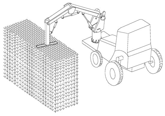
Figure 1.
Manipulator trimming model.
The manipulator is installed on a boss 300 mm from the ground at the front of the tractor, and the driver moves forward at a certain speed to trim the hedges. According to the distance between the inner wheel and the hedge, the wheelbase of the tractor, the installation height and the trimming range, etc., the limit position analysis in AutoCAD is carried out, and the link lengths are 300 mm, 1190 mm, 1037 mm, 330 mm, respectively.
2.2. Hydraulic Drive System of the Manipulator
Considering the problems of simple structure, fast response, low cost, etc., this article adopts valve-controlled hydraulic drive. The system flow is controlled by a servo valve, and the oil is supplied through a hydraulic power source; the system mainly includes hydraulic pumps, electro-hydraulic servo valves, a hydraulic motor, hydraulic cylinders, etc. The hydraulic motor drives the first joint for rotation, and the hydraulic cylinders respectively drive the other joints for pitching. The oil circuit of the hydraulic system is shown in Figure 2.
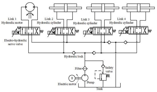
Figure 2.
Scheme of hydraulic drive system.
Taking hydraulic cylinder drive as an example, the control scheme of the system is as follows: the controller controls the spool opening and displacement direction of the electro-hydraulic servo valve through the voltage signal to regulate the output flow and pressure to control the extension or retraction of the piston rod of the hydraulic cylinder. The output force of the hydraulic cylinder is used to provide the torque needed to drive the joint. Finally, the joint angle can be controlled. Angle position sensors are installed at the joints to feedback the joint angle signals to the controllers. The control diagram of hydraulic manipulator system is shown in Figure 3.
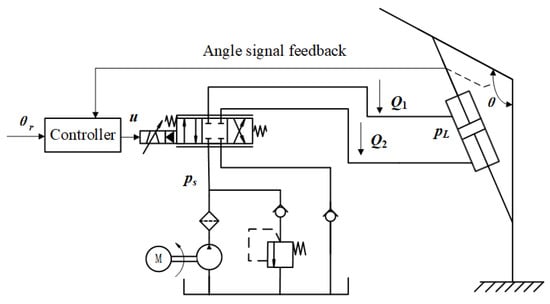
Figure 3.
Control diagram of hydraulic manipulator system.
3. Kinematic Analysis of the Manipulator
3.1. Kinematic Analysis
Kinematics analysis mainly studies the relationship between the joint variables and the pose of the end-effector in space, including forward kinematics inverse kinematics.
Forward kinematics determine the pose of the end-effector based on the given joint variables. In this paper, the D-H method is adopted to establish the link coordinate systems, as shown in Figure 4, where, is the joint angle and is the coordinate system of each link. The homogeneous transformation matrix is defined [21]:
where, and represent the orientation and position of {i − 1}th frame with respect to the {i}th frame.
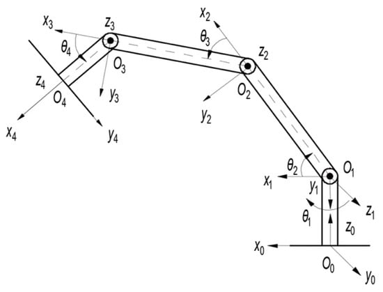
Figure 4.
Setting of the manipulator coordinate system.
By multiplying the matrix from the base frame to the end frame, the pose of the end effector is obtained, that is, the forward kinematics equation:
In Equation (2), .
The main purpose of inverse kinematics is to solve the joint variables according to the given pose of the end-effector. In this paper, the algebraic method is utilized to solve the joint variables as:
In Equation (3), , , .
3.2. Trajectory Planning
Before the manipulator performs the hedge trimming task, it is necessary to plan the trajectory of each joint to facilitate subsequent control. According to the given initial joint angle and target angle, the quintic polynomial interpolation function is adopted to obtain the joint trajectory. The general form is as follows:
In order to make the manipulator move more smoothly, the constraints are set as:
where is the termination time, , are the initial and target joint angles, and and are the joint velocity and acceleration, respectively.
The joint angle corresponding to the target position of the manipulator can be obtained using an inverse kinematics algorithm according to the target pose. The trajectory planning is divided into two working conditions: trimming the top and trimming the side. We can assume that the position coordinates of the target points are (1050, −300, 1700) and (1050, 480, 500) respectively. Substitute Equation (5) for Equation (4) to obtain the trajectory of each joint as follows.
Trimming the top:
Trimming the side:
4. Hydraulic Manipulator System Modeling and Controller Design
4.1. Mathematical Model of the Manipulator System
The simplified model of the 4-DOF manipulator is shown in Figure 5, where, , , , , , , , are the link lengths and joint angles and , , , , , are installation distances (from the installation position to the corresponding joint) of the hydraulic cylinders. We assume that the masses of the links are concentrated at the end; they are , , , respectively.
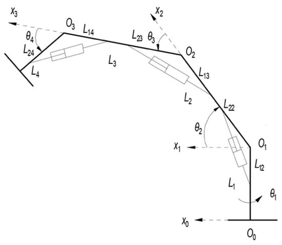
Figure 5.
Simplified model of the manipulator.
According to Lagrange principle [22], the dynamic equation of the 4-DOF manipulator is as follows:
where, respectively denote the position, velocity and acceleration of the joint, is the inertial array of the manipulator, is the centrifugal and Coriolis matrix and is the gravity matrix. denotes the multiple friction forces, is the external disturbance and denotes the torque of each link.
4.2. Mathematical Model of the Hydraulic System
The mathematical model of the hydraulic system mainly includes the fluid flow of the valve, the input and output flow of the cylinder (motor) and the piston dynamics [23]. The valve-controlled hydraulic cylinder model is shown in Figure 6; the derivation process of the kinematics equation is as follows.
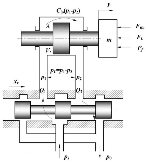
Figure 6.
Valve-controlled hydraulic cylinder model.
The linearized flow equation of the valve is:
where , is the displacement of the servo valve spool, is the valve gain, is the input voltage, is the load pressure, is the flow gain of the servo valve and is the valve flow-pressure gain.
Ignoring the external leakage, the flow continuity is:
where denotes the effective working area of the piston, denotes the leakage coefficient in the cylinder, represents the working volume of the cylinder and is the effective bulk modulus. represents the displacement of the piston, and the nonlinear transformation between it and the joint angle can be obtained from Figure 5:
When the spool of the servo valve begins to move, a pressure difference between the two chambers of the cylinder will be generated, causing the piston position to change. The force generated on the cylinder is obtained using Newton’s second law [24]:
where is the mass of the piston, is the viscous damping coefficient, is the load force and is the friction force, which is composed of static friction, Coulomb friction, viscous friction and Strobeck effect [25].
4.3. Dynamic Coupling Equation of the Hydraulic Manipulator System
The relationship between cylinder thrust and joint torque can be obtained by the principle of virtual work [26]:
where and denote the incremental changes in the joint angle and cylinder displacement, respectively. Therefore, we can obtain:
where represents the Jacobian matrix between the manipulator and the hydraulic system. It is defined as:
Combining Equations (9)–(14), we can obtain the relationship between the control voltage u of the hydraulic system and the driving torque of the manipulator joint:
Therefore, the coupling dynamic equation of the hydraulic manipulator is:
4.4. Design of ANFIS Self-Tuning PID Controller
4.4.1. Fuzzy PID Controller
The hydraulic manipulator system studied in this paper is relatively complex, with high nonlinearity and uncertainty, it is hard to establish a mathematical model accurately, so that the conventional PID control cannot achieve the ideal control effect. Therefore, the fuzzy logic algorithm with nonlinear linguistic mapping, fuzzy inference and strong robustness is combined with the PID controller to adjust PID parameters.
As demonstrated in Figure 7, the FPID controller has two inputs: error (between the desired joint angle and the actual joint angle) and error change rate . Both the input signals are transformed into fuzzy values and in the fuzzy universe. Then, the increments of the PID parameters, can be obtained through fuzzy inference. The increments here are fuzzy variables, which need to be clarified and finally added to the initial values of PID parameters.
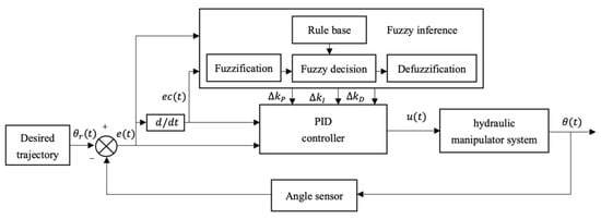
Figure 7.
Structure of fuzzy PID controller.
In this paper, the fuzzy subsets of E, EC, are , which represent negative large, negative medium, negative small, zero, positive small, positive middle and positive large, respectively. According to the design requirements, the domain scopes of , are [−6 6], [−3 3], [−3 3], [−0.03 0.03], [−0.6 0.6], respectively. The membership functions of all parameters are set in gaussian function, and the fuzzy control rule table can be obtained according to the tuning principles of PID parameters and expert experience.
4.4.2. Design of ANFIS-PID Controller
The membership function in FPID control is strongly dependent on expert knowledge and experience; it lacks self-learning and adaptive abilities. Therefore, this paper introduces the learning ability of neural network into the fuzzy inference system, uses ANFIS to adaptively learn, adjusts the membership function and finally adjusts PID parameters to form an ANFIS self-tuning PID controller.
ANFIS is a fuzzy inference system based on the Takagi-Sugeno model. It implements three basic processes of fuzzy controller: fuzzification, fuzzy inference and defuzzification using a neural network. It adjusts membership functions and generates fuzzy rules automatically by training input and output data [27]. For a Sugeno-type fuzzy inference system with two inputs and one output, if-then rules can be expressed as follows:
If is and is , then .
Where, , are input variables, , are the fuzzy linguistic sets corresponding to the inputs for the rule and is the output of the rule.
The ANFIS designed in this paper calculates continuously changing PID parameters according to the error e and error change rate etc. Its network structure consists of five layers, as shown in Figure 8. Each layer is explained below.
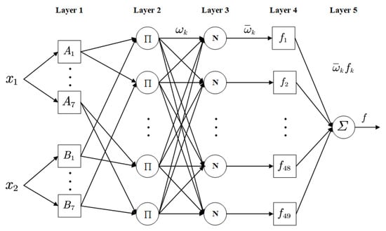
Figure 8.
Structure of ANFIS with two inputs, one output.
Layer 1: In the first layer, each node is an adaptive node with a node function:
where , are the inputs to node ; are the linguistic labels for inputs, with the number set to 7, respectively, and is the output of the node, that is, the membership grade of fuzzy set A (say ). The membership function selected in this paper is Gaussian function [28]:
where, and are referred as premise parameters.
Layer 2: In the second layer, rules are generated, so there are 49 nodes. Each node is a fixed node, and its output represents the firing strength of a rule which is the algebraic product of all inputs:
Layer 3: In the third layer, each node is a fixed node and the firing strength of each rule is normalized by calculating the corresponding rule’s firing strength to the sum of all rules’ firing strengths:
Layer 4: In the fourth layer, each node is an adaptive node, calculating the contribution of the rule to the overall output:
where is the output of layer 3, , , are referred to as consequent parameters.
Layer 5: In the fifth layer, the single node is a fixed node that calculates the overall output for all the inputs.
In this paper, a hybrid learning algorithm that combines the least-squares and backpropagation algorithms is utilized. The least-squares method is used to train the consequent parameters, and the error signals of the output layer are iteratively calculated. Then, the premise parameters are updated according to the error backpropagation algorithm, and the modifiable parameters are adjusted so that the system can better simulate the given sample data.
5. Simulation Results and Analysis
In this section, the trajectory tracking performance of the proposed controller is discussed. The controller is applied to the hydraulic manipulator shown in Figure 1; each link adopts a separate controller. Taking the working condition of trimming the top as an example, the trajectory tracking control is studied, and the expected trajectory is obtained from Equation (6). The simulation is implemented by MATLAB/Simulink (Ver. R2018a) on a personal computer, and the Simulink model is shown in Figure 9. The sampling time and simulation time are set at 1 ms and 10 s, respectively.
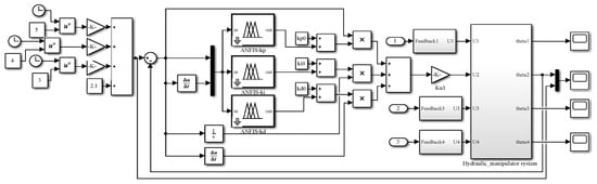
Figure 9.
Simulation model of the ANFIS-PID control system.
In order to prove the superiority of the ANFIS-PID controller, its performance is compared with FPID and PID controllers. Through the simulation experiment, the trajectory tracking curve of each link controlled by the above three controllers is obtained, as shown in Figure 10. Figure 11 is the error graph between the actual trajectory and the expected trajectory. As we can see from the figures, all three control methods can make the system reach the final stable state. When controlled by PID controller, the overshoot of the system is relatively large, which leads to the poor stability of the system. Each link tracks the expected trajectory at about 2.1, 2.5, 2.2, 2.0 s, respectively. The tracking speed is slow and the tracking error is large. Although the FPID controller can reduce the overshoot of the system, its tracking error is large, and the tracking speed is still not fast enough. Compared with other controllers, the ANFIS-PID controller has a smaller angular displacement tracking error and a smaller overshoot, and can quickly track the desired trajectory. In addition, the system is more stable. Therefore, the ANFIS-PID controller can better accomplish the angular displacement tracking task of the manipulator.
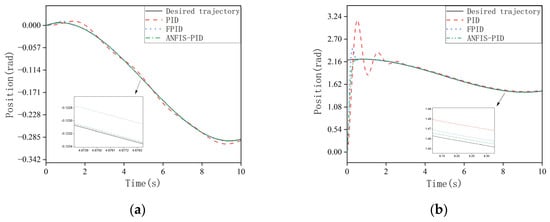
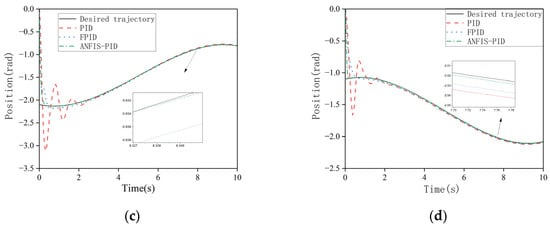
Figure 10.
(a) Trajectory tracking for joint 1; (b) trajectory tracking for joint 2; (c) trajectory tracking for joint 3; (d) trajectory tracking for joint 4.
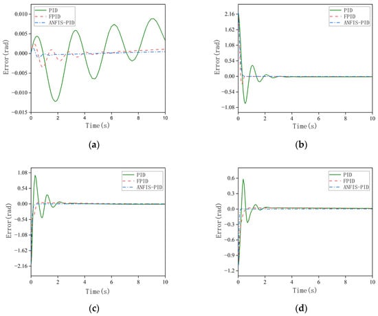
Figure 11.
(a) Angular displacement error for joint 1; (b) angular displacement error for joint 2; (c) angular displacement error for joint 3; (d) angular displacement error for joint 4.
In order to reflect the trajectory tracking effect more clearly and accurately, the trajectory tracking error of Figure 11 is quantified, and the mean absolute error and root mean square error of the actual trajectory of each joint are calculated separately, as shown in Table 1. The quantitative analysis shows that the mean absolute errors of the ANFIS-PID controller proposed in this paper are 0.36%, 0.88%, 0.63% and 0.86% of the PID controller, and 1.82%, 2.96%, 1.99% and 1.67% of the fuzzy PID controller, respectively. Similarly, the root mean square error of the ANFIS-PID controller is 0.56%, 0.90%, 0.69% and 1.10% of the PID controller and 2.81%, 2.99%, 2.16% and 2.11% of the fuzzy PID controller, respectively. The above analysis also proves that the control method proposed in this paper can obtain higher control accuracy compared with PID and fuzzy PID methods.

Table 1.
Mean absolute error and root mean square error of trajectory tracking for each joint.
6. Conclusions
In this paper, an ANFIS-PID controller is proposed and applied to a four-degrees-of-freedom hydraulic manipulator to improve the trajectory tracking accuracy of the manipulator. Firstly, the mechanical structure and the hydraulic drive system of the hydraulic manipulator are designed; secondly, the forward and inverse kinematics of the manipulator are analyzed, the trajectory curves are obtained by the fifth polynomial interpolation function and the connection between the hydraulic system and the manipulator system is derived according to the principle of virtual work, so as to establish the coupled dynamics equations of the hydraulic manipulator system. Finally, for the uncertainty and nonlinearity of the hydraulic manipulator system, the ANFIS-PID controller is designed, the adaptive regulation of the PID parameters is accomplished using the autonomous learning and fuzzy reasoning ability of ANFIS and the simulation is analyzed in Matlab/Simulink. In addition, the PID and fuzzy PID controllers are applied to the manipulator in a simulation for comparative performance analysis. The simulation results show that the ANFIS-PID controller has a smaller tracking error, higher control accuracy and better control effect in trajectory tracking compared with the PID and fuzzy PID controllers; this is in accordance with expectations.
Author Contributions
J.H.: Conceptualization, Supervision, Methodology. F.W.: Software, Writing, review and editing, Validation, Data curation. C.S.: Formal analysis, Software, Writing original draft. All authors have read and agreed to the published version of the manuscript.
Funding
This research was funded by the foundation of Science and Technology Program of Jiangsu Province, funding number: SZ-YC202165.
Institutional Review Board Statement
Not applicable.
Informed Consent Statement
Not applicable.
Data Availability Statement
Data is unavailable.
Acknowledgments
The authors would like to thank Xia Changgao at Jiangsu University for their valuable suggestions and help. The work was supported by foundation of Science and Technology Program of Jiangsu Province (No: SZ-YC202165).
Conflicts of Interest
The authors declare no conflict of interest.
References
- Baek, J.; Jin, M.; Han, S. A new adaptive sliding-mode control scheme for application to robot manipulators. IEEE Trans. Ind. Electron. 2016, 63, 3628–3637. [Google Scholar] [CrossRef]
- Zhang, L.Y.; Liu, L.Z.; Wang, Z.; Xia, Y.Q. Continuous finite-time control for uncertain robot manipulators with integral sliding mode. Inst. Eng. Technol. 2018, 12, 1621–1627. [Google Scholar] [CrossRef]
- Guan, C.; Pan, S.X. Nonlinear adaptive robust control of single-rod electro-hydraulic actuator with unknown nonlinear parameters. Trans. Control Syst. Technol. 2008, 16, 434–445. [Google Scholar] [CrossRef]
- Guo, K.; Wei, J.H.; Tian, Q.Y. Nonlinear adaptive position tracking of an electro-hydraulic actuator. J. Mech. Eng. Sci. 2015, 229, 3252–3265. [Google Scholar] [CrossRef]
- Cui, Y. Study on Hydraulic Robot Actuator Control based on Fuzzy Algorithm; Harbin University of Science and Technology: Harbin, China, 2016. [Google Scholar]
- Zeng, Z.L.; Wu, Y.P.; Li, W.X. Synthetical modeling and fuzzy control simulation of a manipulator-hydraulic drive system. J. Heilongjiang Inst. Sci. Technol. 2004, 14, 96–99. [Google Scholar]
- Sharma, R.; Rana, K.P.S.; Kumar, V. Performance analysis of fractional order fuzzy PID controllers applied to a robotic manipulator. Expert Syst. Appl. 2014, 41, 4274–4289. [Google Scholar] [CrossRef]
- Krishna, S.; Vasu, S. Fuzzy PID based adaptive control on industrial robot system. Mater. Today Proceeding 2018, 5, 13055–13060. [Google Scholar] [CrossRef]
- Jin, X.; Chen, K.; Zhao, Y.; Ji, J.T.; Jing, P. Simulation of hydraulic transplanting robot control system based on fuzzy PID controller. Measurement 2020, 164, 108023–108031. [Google Scholar] [CrossRef]
- Hao, W.R.; Kan, J.M. Application of self-tuning fuzzy proportional-integral-derivative control in hydraulic crane control system. Adv. Mech. Eng. 2016, 8, 1687814016655258. [Google Scholar] [CrossRef]
- Er, M.J.; Sun, Y.L. Hybrid fuzzy proportional-integral plus conventional derivative control of linear and nonlinear systems. Trans. Ind. Electron. 2001, 48, 1109–1117. [Google Scholar]
- Yang, Y.; Zhang, Q.J. Design of self-optimizing FPID controller with particle swarm algorithm. Electr. Autom. 2018, 201–204. [Google Scholar] [CrossRef]
- Kumar, N.; Rani, M. Neural network-based hybrid force/position control of constrained reconfigurable manipulators. Neurocomputing 2021, 420, 1–14. [Google Scholar] [CrossRef]
- Kang, E.; Qiao, H.; Gao, J.; Yang, W.J. Neural network-based model predictive tracking control of an uncertain robotic manipulator with input constraints. ISA Trans. 2020, 109, 89–101. [Google Scholar] [CrossRef]
- Jin, J.; Gong, J.Q. An interference-tolerant fast convergence zeroing neural network for dynamic matrix inversion and its application to mobile manipulator path tracking. Alex. Eng. J. 2021, 60, 659–669. [Google Scholar] [CrossRef]
- Liu, C.X.; Zhao, Z.J.; Wen, G.L. Adaptive neural network control with optimal number of hidden nodes for trajectory tracking of robot manipulators. Neurocomputing 2019, 350, 136–145. [Google Scholar] [CrossRef]
- Yang, Z.Q.; Peng, J.Z.; Liu, Y.H. Adaptive neural network force tracking impedance control for uncertain robotic manipulator based on nonlinear velocity observer. Neurocomputing 2019, 331, 263–280. [Google Scholar] [CrossRef]
- Jang, J.S.R. ANFIS: Adaptive-network-based fuzzy inference system. IEEE Trans. Syst. Man Cybern. 1993, 23, 665–685. [Google Scholar] [CrossRef]
- Abderrahim, B.; El Houssine, E.C.M.; Hassan, S.; Hicham, A.E.; Bouras, A. Intelligent ANFIS controller of two cooperative 3-DOF manipulators: The case of manipulation under non-slip constraints. In Proceedings of the 2022 2nd International Conference on Innovative Research in Applied Science, Engineering and Technology (IRASET), Meknes, Morocco, 3–4 March 2022; pp. 1–7. [Google Scholar]
- Lazreg, M.; Benamrane, N. Hybrid system for optimizing the robot mobile navigation using ANFIS and PSO. Robot. Auton. Syst. 2022, 153, 104114. [Google Scholar] [CrossRef]
- Lee, D.; Seo, T.; Kim, J. Optimal design and workspace analysis of a mobile welding robot with a 3P3R serial manipulator. Robot. Auton. Syst. 2011, 59, 813–826. [Google Scholar] [CrossRef]
- Kumar, V.; Rana, K.P.S.; Kler, D. Efficient control of a 3-link planar rigid manipulator using self-regulated fractional-order fuzzy PID controller. Appl. Soft Comput. J. 2019, 82, 105531. [Google Scholar] [CrossRef]
- Ding, W.H.; Deng, H.; Xia, Y.M.; Duan, X.G. Tracking control of electro-hydraulic servo multi-closed-chain mechanisms with the use of an approximate nonlinear internal model. Control Eng. Pract. 2017, 58, 225–241. [Google Scholar] [CrossRef]
- Yousif, H.M.; Ganesh, K. Internal type-2 fuzzy position control of electro-hydraulic actuated robotic excavator. Int. J. Min. Sci. Technol. 2012, 22, 437–445. [Google Scholar]
- Yuan, F. Optimization Design of Cam-Robot Hydraulic Servo Motor; Shanghai Jiao Tong University: Shanghai, China, 2017. [Google Scholar]
- Kim, J.; Jin, M.; Chio, W.; Lee, J. Discrete time delay control for hydraulic excavator motion control with terminal sliding mode control. Mechatronics 2019, 60, 15–25. [Google Scholar] [CrossRef]
- Zhang, X.J. Study on the adaptive network-based fuzzy inference system ans simulation. Electron. Des. Eng. 2012, 20, 11–13. [Google Scholar]
- Jiang, K.; Zhang, T.; Feng, Z.X. AN ANFIS-PID control strategy for a semi-active suspension with magneto rheological damper. Modul. Mach. Tool Autom. Manuf. Tech. 2016, 4, 80–83. [Google Scholar]


Disclaimer/Publisher’s Note: The statements, opinions and data contained in all publications are solely those of the individual author(s) and contributor(s) and not of MDPI and/or the editor(s). MDPI and/or the editor(s) disclaim responsibility for any injury to people or property resulting from any ideas, methods, instructions or products referred to in the content. |
© 2023 by the authors. Licensee MDPI, Basel, Switzerland. This article is an open access article distributed under the terms and conditions of the Creative Commons Attribution (CC BY) license (https://creativecommons.org/licenses/by/4.0/).