Development of Automatic Electric Drive Drilling System for Core Drilling

Abstract

Core drilling has been widely used in mineral exploration with diamond-impregnated drilling technology. Automation is a critical technology in improving core drilling efficiency and reducing core drilling costs, but there is no complete automation that can control the entire core drilling process. In this paper, an electric drive laboratory drilling system was established using programmable logic controller (PLC) technology. A proportional integration differentiation (PID) control algorithm was developed to achieve closed-loop control of the weight-on-bit (WOB) during the drilling process. Four drilling modes were developed for the drilling system, and their performances were verified by drilling test. A constant-speed mode is proposed as the most suitable mode for the system. The recommended rate of penetration (ROP) of the rock sample and bit used in the experiment was obtained through the power optimization drilling test. The results show that the optimal rotation speed ranged from 700 to 1000 rpm, and the optimal ROP ranged from 2.0 to 2.6 m/h.

1. Introduction

Drilling systems have been used in various fields, such as mineral exploration, the development of oil and gas resources, underground water development, and geothermal power. As a necessary means of resource exploration, core drilling plays an essential role in resource exploitation and economic development. However, core drilling is characterized by miniaturization, a low degree of automation, low profits, and high labor intensity [1,2]. Most well drilling costs are not product-cost-dependent but time-dependent. Therefore, the main goals of core drilling optimization are to reduce the total time and labor intensity [3,4]. Drilling speed, commonly called the rate of penetration (ROP), becomes a key performance indicator. ROP optimization involves selecting the operational parameters to improve the drilling speed in this case. Rock formation, hole diameter, hole cleaning and hydraulics, weight-on-bit (WOB), rotational speed (RPM), and bit type are the six factors that influence ROP [5]. Instead of choosing a suitable drill bit and drilling fluid type before drilling, a new solution relies on real-time analysis to optimize the operational parameters, WOB and RPM, during drilling. Intelligent and automatic drilling systems suggest operational parameters for drillers by correlating real-time drilling data with vast amounts of historical data stored in a database, or by exerting complete control of all rig equipment with significant decision points. The latter describes the levels of automation that are likely years away from deployment in the field. Developing a drilling system under laboratory conditions will contribute to research on automated drilling and drilling rate optimization in the core drilling field [6,7,8,9,10]. The drilling systems automation technical section of the Society of Petroleum Engineers (DSATS) developed a DSATS drillbotics program. The program is an international competition for universities to design and build a small drilling rig for petroleum and gas automation. However, it is hard to find automation in core drilling.

Compared with petroleum and gas drilling, core drilling has the characteristics of small equipment volume, small bore diameter, fast construction time, and low economic benefits; thus, core drilling has a low level of automation. Owing to the poor working environment of core drilling and drilling rig product molding, the drive mode of the core drilling rig is generally a hydraulic or mechanical drive. The hydraulic drill rig has the disadvantages of complicated maintenance, high cost, and poor delay control, but it has the advantages of large WOB and large torque. The electric drive drill has the advantages of simple structure and high control accuracy, but it has the disadvantages of large volume. Wang et al. developed a multiparameter hydraulic submersible hammer test platform to achieve drilling through hydraulic drive [11]. Zhao developed a multifunction hydraulic drilling test platform [12]. In addition, the Commonwealth Scientific and Industrial Research Organisation (CSRIO) transformed a power head drill rig into an intelligent real-time formation identification system, which is equipped with a parameter monitoring console. The system can analyze real-time rig parameters, infer bit status, and identify formation information. The electric drive core drilling system can simulate actual drilling, provide the measurement and recording of various drilling parameters, provide the basis for improving drilling technology, develop drilling equipment, and provide ideas for drilling optimization [13,14]. The key goal of drilling automation at this stage is to develop digital and robust tools to assist drillers in critical phases and, if possible, to automate routine tasks that machines can easily control [15]. IRI and NOV (Houston, TX, USA), Dreco (Edmonton, AB, Canada), Hitec (Sola, Norway), Siemens (Munich, Germany), and others have developed rig systems with AC frequency conversion as the driving force. However, the large-scale equipment used at the petroleum and gas industry application level is not suitable for laboratory experiments. In terms of electric drive drilling system, Liu developed a miniature drilling device with a drilling parameter acquisition module, but the device did not realize closed-loop control in the drilling process [16]. Joseph Paez Chavez set up an experimental device to study the stick–slip phenomenon in drilling with DC top drive. However, the WOB and torque provided by the device are limited [8]. Real F.F. et al. built a drilling experiment device to explore the stick–slip characteristics of drilling tools in the process of drilling with electric jacks. However, in the actual process of drilling, the motor speed oscillated significantly and could not provide a stable rotation speed [9]. Magomed K et al. developed an automatic drilling system, which is powered by a small top drive hollow shaft DC motor [7]. It is equipped with a measuring-while-drilling module to realize automatic drilling control, but the motor’s power is not enough to complete drilling experiments at real drilling level.

In summary, most of the current laboratory drilling systems are driven by hydraulic hybrid drive or a pure hydraulic system, and the development of electric drive is lagging. Moreover, laboratory drilling systems with pure electric drive mostly provide very limited WOB and torque, which are only used for specific experiments. In addition, most of the control of drilling parameters is based on the feedback control between people and sensors, which does not realize the real sense of automatic control. Most laboratory drilling systems with well-designed control systems are not capable of drilling at real size, especially for core drilling, which is unable to restore actual drilling.

The main objective of this study is to develop an electric driven laboratory core drill rig, and to develop a supporting automatic drilling control system to meet the requirements of simulating actual core drilling engineering. The system can perform simple drilling experiments with four drilling modes, record drilling data, and optimize the ROP for energy consumption.

In this paper, the basic theory of drilling is introduced. Then, the drilling system design, including the hardware and software system, is presented. Subsequently, four control modes are introduced and verified by experiments, and the rate of penetration is optimized by power optimization. Finally, the results and discussion are presented to demonstrate the performance of the proposed automation drilling system.

2. Modeling and Theory

A drilling rig is composed of a variety of machines and equipment, with a variety of functions regarding the joint working unit. It is mainly composed of a rotation system, circulation system, and hoisting system. There are many undetermined factors in the drilling process, such as the concealability and complexity of the formation and the operation characteristics of the drilling rig, which can cause harmful vibration impact on the rotation system of the drilling rig.

ROP is the core of drilling, and the commonly used empirical model from Bourgoyne and Youngs [17] is

$$\begin{array}{l}\mathrm{ROP}=\exp [a_1+a_2(3048-\mathrm{TVD})+a_3{\mathrm{TVD}}^{0.69}(g_p-1.078)\\ +a_4\mathrm{TVD}(g_p-\mathrm{ECD})+a_5(\frac{\mathrm{RPM}}{60})+a_6(-h)\\ +a_7\frac{\rho q}{350\mu d_n}+a_8\ln [\frac{\frac{\mathrm{WOB}}{d_b}-{(\frac{\mathrm{WOB}}{d_b})}_t}{0.7-{(\frac{\mathrm{WOB}}{d_b})}_t}]]\end{array}$$

(1)

where a₁–a₇ are the empirical coefficients of formation, well depth, well pressure, drill bits and fluid; TVD is well depth; g_p is pore pressure gradient of the formation; ECD is equivalent circulating mud density at the hole bottom; ρ is mud density; μ is the apparent viscosity at 10,000 s⁻¹; d_n is bit nozzle diameter; d_b is bit diameter. Although all the terms in the formula are empirical values, it is obvious that WOB and RPM are two important quantities.

The current study of a drill string motion model can be summarized as a spring mass damping system, which simplifies the whole drill string motion process into a single degree of freedom or multidegree of freedom system model, and the interaction model between drill bit and rock is introduced as the lower boundary condition. Based on these factors, the basic dynamic equation of the system is established. By solving the basic equations of the system dynamics, the variables describing the dynamic characteristics of the system are obtained [18,19].

Generally, the drill string system of a drilling rig can be described as a torsional pendulum [20,21]. The main components are two mechanical devices with attenuated inertia, connected by an elastic drill pipe [22].

Table 1. Parameters and variables characterizing the rotation system.

Number	Parameter	Definition	Units
1	φ	Angular displacements between φr and φb	rad
2	φr	Angular displacement of power head	rad
3	φb	Angular displacement of drill bit	rad
4	Jb	Moment of inertia of drill bit	$\mathrm{kg}\cdot {\mathrm{m}}^2$
5	$\dot{{\phi }_b}$	Angular velocity of drill bit	rad/s
6	$\ddot{{\phi }_b}$	Angular acceleration of drill bit	rad/s2
7	C1	Attenuation coefficient of drill string	$\mathrm{N}\cdot \mathrm{m}\cdot \mathrm{s}/\mathrm{rad}$
8	Ttob	Nonlinear friction torque of bit torque	$\mathrm{N}\cdot \mathrm{m}$
9	K	Torsional stiffness coefficient of drill string	$\mathrm{N}\cdot \mathrm{m}/\mathrm{rad}$
10	Jr	Equivalent moment of inertia of power head	$\mathrm{kg}\cdot {\mathrm{m}}^2$
11	Jm	Moment of inertia of motor	$\mathrm{kg}\cdot {\mathrm{m}}^2$
12	Jrot	Moment of inertia of power head	$\mathrm{kg}\cdot {\mathrm{m}}^2$
13	C2	Attenuation coefficient of power head	$\mathrm{N}\cdot \mathrm{m}\cdot \mathrm{s}/\mathrm{rad}$
14	u	Unit step input	$\mathrm{N}\cdot \mathrm{m}$
15	${\mathsf{\Omega }}_{ref}$	Given speed of bit	rad/s
16	Tm	Motor driving moment	$\mathrm{N}\cdot \mathrm{m}$
17	Trob(dyn)	Moment of dynamic friction	$\mathrm{N}\cdot \mathrm{m}$
18	α1, α2, α3	Empirical coefficient of drilling

shows the parameters used in the model of the rotation system.

In most of the literature, the downhole mechanism is considered as a completely rigid body, and the drill string (drill pipes and extensions) is considered as a torsion spring with stiffness depending on the drill string parameters [20].

As shown in Figure 1, the main components of the model are two damped inertias [23]. It is assumed that the drill pipe is of the same mass and the whole length is simply considered as a single linear spring system, with an elastic coefficient of K and no lateral motion.

The mathematical model of drilling can be described by the motion equation of the drilling tool in downhole part, the motion equation of the driving system in overground part, and the friction equation of the bit.

(1)

Equation of motion of the downhole part

According to the assumption that the drill string moves similar to a torsional pendulum, the drill pipe is equivalent to a torsional spring, the power head rotates at a constant speed, and the drill collar is stiff. The equation of motion of downhole part is

$$J_b{\ddot{\phi }}_b+C_1{\dot{\phi }}_b-K\phi =-T_{tob}({\dot{\phi }}_b)$$

(2)

(2)

Equation of motion of the drive system

The mechanical system characteristics of the drive system consist of three parts: the power head, the gearbox, and the motor. The equation of motion of the system is:

$$\begin{array}{l}{J}_r{\ddot{\phi }}_r+C_2{\dot{\phi }}_r+K\phi =T_m\\ C_2{\mathsf{\Omega }}_{ref}+u=T_m\end{array}$$

(3)

where $J_r=J_{rot}+n^2{J}_m$.

(3)

Equation of friction moment

Drilling is limited by the conditions of the downhole part. Because the static friction coefficient of the drill string is greater than the sliding friction coefficient, the torque of the drill pipe storage energy will convert the energy of inertia of the drill string. Then, the speed of the bit will be beyond the steady speed. In this condition, the rotational speed is in critical condition, the interaction of rock and bit will produce harmful vibrations.

Torsional vibrations are considered as the most dangerous vibrations to which the drill string is vulnerable. The phenomenon responsible for the regeneration of these vibrations is known as ‘stick–slip’. Stick–slip occurs when the drill bit is frictionally engaged with the formation in a nonlinear manner [24]; it makes the whole drill pipe slide or stop moving. However, if the accumulated torsional energy reaches a certain level, the drill will be released suddenly and will rotate at a high speed. The resulting torsion wave will be passed to the running at the top of the rotation system. However, because the power head has strong inertia, it can hold the drill pipe in place, so that the torsion wave returns to the bit through the drill pipe. In this way, the bit will stall again, and the torque wave will repeat, which causes a very large and harmful vibration around the drill pipe. If out of control, the drill pipe and the drill bit will be damaged together.

In the two-degree-of-freedom (2-DOF) model of the drilling rig rotation system, the friction torque is simply considered as the sum of the counter torque of the drill bit and the nonlinear friction torque on the drilling bottom device.

The bit velocity function can be given by the nonlinear function of Equation (4):

$$T_{tob}({\dot{\phi }}_b)=T_{tob(dyn)}\frac{2}{\pi }({\alpha }_1{\dot{\phi }}_b\exp (-{\alpha }_2\left|{\dot{\phi }}_b\right|)+\arctan ({\alpha }_3{\dot{\phi }}_b))$$

(4)

Equation (4) is used for the nonlinear equations of motion of the rotation system of a drilling rig with 2-DOF.

(4)

Nonlinear equation of the drilling system

The nonlinear state space representation of the rotary drilling system is

$$\begin{array}{l}\dot{x}(t)=f[x(t)]+g(x)u(t)\\ y(t)=h[x(t)]\end{array}$$

(5)

where the state vector is $x(t)={[x_1,x_2,x_3]}^T={[{\dot{\phi }}_b,\phi ,{\dot{\phi }}_r]}^T\in R^3$, and the measured output variable is $y(t)\in R$.

$$\begin{array}{c}f(x)=\left[\begin{array}{c}-b_1{\dot{\phi }}_b+c_1\phi -d_1{T}_{tob}({\dot{\phi }}_b)\\ {\dot{\phi }}_r-{\dot{\phi }}_b\\ -b_2{\dot{\phi }}_r-c_2\phi +d_2{\mathsf{\Omega }}_{ref}\end{array}\right]\\ \\ g(x)={[\begin{array}{ccc}0& 0& d_2\end{array}]}^T\\ \\ \begin{array}{c}{b}_1=C_1/J_b,c_1=K/J_b,d_1=1/J_b\\ b_2=C_2/J_r,c_2=K/J_r,d_2=1/J_r\\ \phi ={\phi }_r-{\phi }_b\end{array}\end{array}$$

(6)

If the control object of the control system is nonlinear, linearity control techniques generally fail to produce the desired performance, especially for the control system with high precision requirements.

The exact linearization method is a nonlinear control design method [25,26]. Exact linearization can turn an affine nonlinear system to a linear system by choosing adequate diffeomorphisms and nonlinear feedback control. The basic principle of this method is that the dynamic characteristics of the nonlinear system can be converted into linear dynamic characteristics (in whole or in part) through appropriate feedback transformation and nonlinear transformation, so that the exact linearization of input–state and input–output can be realized [27,28,29].

Finally, the problem of complex nonlinear system is transformed into a linearized problem, so the familiar linear control method can be used for design [30,31,32].

An output must be selected to make the system feasible feedback linearization, so the output turns out to be the angular velocity of the downhole part, which is $h(x)={\dot{\phi }}_b$.

If the conditions are satisfied, it is possible to find a scalar function $\varphi (x):U\in R^n$ to satisfy Equation (8), as follows:

$$\begin{array}{l}x(t)=f[x]+g(x)u\\ y(t)=h[x]\end{array}$$

(7)

A control input is then obtained through

$$u=\alpha (x)+\beta (x)\nu$$

(8)

such that the closed-loop system has a new set of variables in linear state:

$$\dot{z}=Az+b\nu$$

(9)

where

$$\begin{array}{ccc}A=\left[\begin{array}{ccccc}0& 1& 0& \cdots & 0\\ 0& 0& 1& \cdots & 0\\ \cdots & \cdots & \cdots & \cdots & \cdots \\ 0& 0& 0& \cdots & 1\\ 0& 0& 0& \cdots & 0\end{array}\right]& ,& B=\left[\begin{array}{c}0\\ 0\\ \cdots \\ 0\\ 1\end{array}\right]\end{array}$$

(10)

A and B are in the canonical form of Brunovski, however, there is no loss of generality.

According to the theoretical basis of input–state linearization control, the linearization method can be used for the mathematical model of the drilling rig rotation system, and the complex nonlinear system can be converted into a linear system [31]. The input–state linearization controller of the 2-DOF drilling rig rotation system is designed through the familiar control method of linear system. It can compensate the harmful vibration caused by the nonlinear characteristics of the rig. According to the nonlinear motion equation state equation and output equation of the drilling rig rotation system given by Equation (6), the bit angular velocity can be obtained by linearization of the state equation.

The first component of state transformation z is

$$z_1={\dot{\phi }}_b$$

(11)

Select other state variables as

$$z_2=L_f{z}_1=-a_1{\dot{\phi }}_b+b_1\phi -c_1{T}_{tob}({\dot{\phi }}_b)$$

(12)

$$z_3=L_f^2{z}_2=H{z}_2+b_1({\dot{\phi }}_r-{\dot{\phi }}_b)$$

(13)

where

$$H=-b_1-d_1[\frac{2T_{tob(dyn)}}{\pi }({\alpha }_1{e}^{-b_2{z}_1}-{\alpha }_1{\alpha }_2{z}_1{e}^{-{\alpha }_2{z}_1}+\frac{{\alpha }_3}{1+{({\alpha }_3{z}_1)}^2})]$$

(14)

resulting in the new state equation:

$$\{\begin{array}{c}{\dot{z}}_1=z_2\\ {\dot{z}}_2=z_3\\ {\dot{z}}_3=M{z}_2^2+H^2{z}_2+H(z_3-H{z}_2)+c_{1}Q+c_1{d}_{2}u\end{array}$$

(15)

where

$$Q=-\frac{b_2}{c_1}(z_3-H{z}_2)-b_2{z}_1+b_1{z}_1-(c_1+c_2)\phi +b_2{\mathsf{\Omega }}_{ref}-d_1{T}_{tob}(z_1)$$

(16)

$$M=\frac{2d_1{T}_{tob(dyn)}}{\pi }[e^{-{\alpha }_2{z}_1}(-2{\alpha }_1{\alpha }_2+{\alpha }_1{\alpha }_2^2{z}_1)-\frac{2{\alpha }_3^3{z}_1}{{(1+{({\alpha }_3{z}_1)}^2)}^2}]$$

(17)

The nonlinear equation of drilling rig rotation system can be deduced as a linear equation, from which the input–state linearization controller can be obtained as

$$u=\frac{1}{c_1{d}_2}[v-M{z}_2^2-H^2{z}_2-H(z_3-H{z}_2)-c_{1}Q]$$

(18)

Based on the linearization of the system line, the rotation system controller of the drilling system is designed. Figure 2 shows the control loop of the whole system.

3. Design and Development

In this study, an automatic electric drive drilling system is proposed. Through the servo motor and servo control system, the system could control the ROP, WOB, and cutting during the drilling process. Compared with the traditional hydraulic rig, this system not only improves the precision of control by introducing a servo motor, but also dramatically improves the system’s reliability, thereby reducing the maintenance time and cost of the device. The overall design of the experimental system includes a hoisting system, rotation system, circulation system, control system, drill string system, data acquisition system, and monitoring system. This section introduces the design, calculation, and system composition of the hardware part of the drilling system in detail.

3.1. Hardware Systems

The drilling system is illustrated in Figure 3 and Figure 4. It consists of four hardware systems: a rotation system, hoisting system, circulation system, and drill string system.

Rotation System: The rotation system is similar to the conventional top drive used for vertical drilling. The rotation system provides torque and speed through a servo motor.

The servo motor of the rotation system was fixed to the frame, and the motor shaft was connected to the upper part of the torque sensor through coupling. The torque sensor measures the actual torque output of the servo motor. The lower part of the torque sensor was connected to the rotary spindle through the splines. Outside the torque sensor, the pressure sensor measures the WOB in real time. The rotary motor is a Delta ASDA-A2 series servo motor, and the communication mode is CANopen. The motor-rated power, torque, and speed were 7.5 KW, 47.5 N·m, and 1500 rpm, respectively. It can satisfy the maximum rotary torque and speed required for regular drilling in the demand analysis.

The servo controller can use analog voltage signals to control the RPM and the torque from the top drive. The signals were transmitted from programmable logic controllers (PLCs) to the servo driver.

The differential equation of the system:

$$J\frac{d^2\theta }{d{t}^2}+B\frac{d\theta }{dt}+k\theta =T$$

(19)

Hoisting System: To simulate drilling operations, the system was equipped with a hoisting system consisting of an actuating motor, reduction box, mounting frame, and gear shaft [33,34,35,36].

The gear shaft of the system was located at the upper part of the base of the device, and the transmission mode was a rack-and-pinion transmission. The shaft is the absolute multiturn encoder at one end of the gear. The encoder measured the footage, bit position, and ROP. The other side of the gear shaft is related to the reducer, which is converted into a WOB through rack and pinion. The reducer is a DYNABOX reducer, a self-locking worm gear reducer with a reduction ratio of 90:1 and a mechanical efficiency of 62%. The servo motor is a three-phase synchronous AC motor with a rated power of 3.65 kW, a torque of 11.7 N·m, and a speed of 3000 rpm. There were two rotating bearings between the gear shaft and frame, and three pairs of ear plates were installed at the bottom of the frame to ensure that the rack was not offset when the frame went up and down.

The servo motor can operate with a rated torque within the rated speed, and the communication mode is Powerlink communication. The high accuracy of the actuating motor is key to ensuring the required weight-on-bit (WOB) control. To address the system’s vibrations challenge, a pinion and racks were used between the actuating motor and actuators to reduce the overall vibrations, thereby making the system sturdier.

The differential equation of the system:

$$J_{\sum }(\frac{n}{r})\frac{d^2{x}_0}{d{t}^2}+c\ast (\frac{n}{r})\frac{d{x}_0}{dt}+K_{\sum }(\frac{n}{r})x_0=K_{\sum }{\theta }_i$$

(20)

where n is the reduction ratio, and r is the radius of the gear indexing circle.

Circulation System: This circulation system provides a large pump volume for mud circulation [31]. This device circulates the drilling fluid (water, water-based mud, or oil-based mud) from the top of the derrick to the drill bit. The circulation system consists of a water box, rotary spindle, core box, self-priming pump, frequency changer, and a mud pool. The rotary spindle was equipped with a pair of water outlets, and the water outlet was placed in a water box. Two waterproof rubber rings were placed in the water box to prevent the washing fluid and mud from entering the bearing pedestal.

During drilling, mud was extracted from the mud pool by a self-priming pump to the water inlet of the water box, and the bit was cooled and lubricated using a rotary spindle. Simultaneously, the cuttings and mud generated during the drilling process settled in the core box, and mud returned to the mud pool from the core box. The maximum pump capacity of the self-priming pump for mud circulation was 50 L/min.

The frequency changer prevents the pumps from overheating, and should change the pump volume by controlling the input voltage and current to realize the stepless adjustment of the pump volume.

Drill String System: The drill string system consists of a pipe, sensors, joint, and impregnated diamond drill bit. The rotary motor shaft was connected to the upper part of the torque sensor through coupling, and the torque sensor measured the actual torque output using a servo motor. The pressure sensor, which measures the WOB, relates to the bearing box with a couple of thrust bearings, and the box relates to the tap to ensure the use of the circulation system. The joint can be changed to connect the drill bits with different diameters. The mechanical angle of the top drive can be varied by pulsing it to change the azimuth angle.

Conventional drilling machines generally control the WOB and RPM to control the drilling state. Owing to the mechanical structure, the system controls the drilling state via the RPM, and the feed speed is equal to the ROP, which means that the system cannot directly control the WOB.

3.2. Software System

Combined with the characteristics of the hardware system, it is necessary to build a software system that includes control, data acquisition, and monitoring systems to explore the algorithm of the automatic drilling function [34]. Referring to the traditional drilling mode, the system developed four drilling modes: constant-pressure, constant-speed, constant-torsion, and constant-power drilling.

3.2.1. Control System Architecture

The control system of the drilling system is key to realizing drilling automation. In this system, the control architecture comprises three layers: PLC in the first, a computer in the second, and cloud data storage based on temporal data in the third.

In the first layer, the control system is used to control the core systems of the rig, such as rotation, hoisting, and circulation systems, with PLC or other controllers. Each system was controlled by a unified PLC that sent instructions to the controllable systems on the rig and collected information from the sensors equipped with each system. In the second layer, the PC handles the decision-making system. This system involves a digital operating client based on Mapp viewHMI, ROP optimization algorithms, drilling incident prediction, carrying out remedial actions, and sending data to a configured database for data analysis and control algorithm optimization (third layer). The critical factor in implementing the control architecture is ensuring that all drilling systems can be remotely controlled. Figure 5 shows the implemented control system data flow with PLCs.

The PLC of the drilling system is a B&R PLC, model X20CP3585, which has an extension I/O and extension bus communication module, and the user can realize a variety of communication and signal acquisitions according to their needs. Port X20AI4632 is the analog quantity acquisition module, and X20DI9371 and X20DO8323 are the digital quantity input and output modules, which are related to the limit switch and emergency stop switch, respectively. X20IF1041 is the CANopen master station module, through which communication with the slave station (rotation system motor and position encoder) is realized. Powerlink interface for the PLC built-in interface to achieve Powerlink communication with the hoisting system motor.

3.2.2. Sensors and Data Flow

Due to core drilling miniaturization characteristics, sensors play an essential role in developing automated drilling systems. Sensors must meet the installation requirements of the drilling system while ensuring that the computer relies on the data provided by the sensors to make decisions and provide valuable advice to the user. Core drilling is challenging to measure during drilling (MWD) owing to its small hole diameter. Instead of MWD, the system uses sensors installed near the bit in the drill string system to monitor the working face torque and WOB in real time.

As shown in Figure 3 and Figure 4, the drilling system has five sensors, including a pressure sensor capable of providing measurements for the central axis, and a torque sensor that measures the torque at the drill string. Drill string vibration is a complex phenomenon formed by the coupling of axial, lateral, and torsional vibration modes. In small-bore vertical drilling, the primary vibration direction can be considered axial; thus, vibration monitoring can be realized by measuring instantaneous changes in the WOB. When the vibration is too large, the operator can adjust the drilling parameters (WOB and RPM) to mitigate the vibration.

In traditional core drilling rigs, core drilling data acquisition has always been a missing link. Because there is no data accumulation in the drilling parameter database, the database can only be expanded through an experiment with the drilling system. In each drilling experiment, the sensors collected the time-stamped data throughout the drill. During each drilling experiment, the sensors collected time-stamped data throughout the drilling process. These data were recorded using a high-frequency data acquisition (DAq) module in real time or post analysis.

The sampling frequency of the PLC acquisition module was 10,000 Hz, and the digital signal collected by the program was recorded and saved at a frequency of 100 Hz. In this process, high-frequency noise is aliased into low-frequency noise owing to the signal aliasing. To determine the cutoff frequency of filtering, the fast Fourier transform of the MATLAB software was used for spectrum analysis of the data collected after the motor was turned on, as shown in Figure 6.

The basic theoretical formula for a low-pass filter is as follows:

$$y(t)=K\ast u(t)+(1-K)\ast y(t-1)=y(t-1)+K\ast [u(t)-y(t-1)]$$

(21)

where K is dT/T, dT is step size, T is the time constant, u(t) is input signal, and y(t) is output signal.

Generally, for a certain controller, its operation period is certain, so only the time constant can be adjusted to change the filtering effect. Therefore, the data sampled in real time were filtered using a 15 Hz low-pass filter and calibrated with zero drift.

The sensor acquisition data of the motor power-off, power-on, and rotation at cutoff frequencies of 5 kHz, 2 kHz, 100 Hz, 50 Hz, 15 Hz, and 1 Hz were collected to verify the filtering effect. The results are shown in Figure 7.

SQL is a computer-based structured query language that is used to store, manipulate, and retrieve data in relational databases. This database system was created using MySQL, a well-known RDBMS. To simplify the data collection process, different data were sampled at different frequencies. The torque and pressure were sampled at a high frequency of 100 Hz, whereas the pump pressure, pump volume, and encoder were sampled at a low frequency of 1 Hz. The MySQL database requires two different databases, one for high-frequency sensor data and the other for low-frequency sensor data. MySQL not only uses the characteristics of the RDBMS, but also provides a good query means for time-stamped data.

To facilitate the management of data stored in the database, a Django-based web client acts as an interface between the user and the database. The collected data can be saved in the CSV format in computer files and stored on the CF card of the PLC as a backup.

According to the core drilling process and the state of the sensor, each data point is defined by eight parameters: drilling time, WOB, RPM, ROP torque, pump rate, pump pressure, and rock type. A user-friendly web application was created to make the data in the database easily accessible. Users can log into the application and manage stored data, and the researcher can tag selected and downloaded data or a specific subset of the data at a particular time.

3.2.3. Software Architecture and Security Function

The software architecture is configured as a multithreaded system with an API based on an open platform communication unified architecture (OPC UA). Using Mapp ViewHMI technology, the system supports remote connectivity and remote event processing and receives data from the rig in real time as required.

Mapp ViewHMI technology is a software developed by B&R for industrial machinery and equipment. The system integrates modules to enable developers to rapidly build a user management system, alarm system, and motion control sequence modules. This technology can easily manage complex algorithms, allowing programmers to focus entirely on machine processes. This technology is compatible with the PLC used in drilling systems, which is conducive for later maintenance and continuous development.

OPC UA is a typical API implementation. The plug-and-play nature of the OPC UA protocol enables it to be used as an API in drilling systems. Therefore, the network client can implement two interaction modes: remote execution of sensor request information and issuing commands to actuators.

The GUI was developed for this laboratory-scale drilling system using Mapp ViewHMI. This visualization GUI monitors the status of the automatic control system and the real-time drilling engineering parameters. GUI is equipped with virtual gauges and parameters that display control system settings and sensor feedback and build measurement curves based on sensor values in real time to help improve drilling engineering parameters.

The system thoroughly considered the safety factors during device operation in this study. The safety functions include the following.

• Triple limit

Three limits are set to prevent the device from exceeding the design stroke. The first is the program limit that is triggered by encoder feedback. The entire device stopped operating when the encoder position value exceeded the limit value. The second limit is the mechanical limit, connected to the DI/DO module through a limit switch. A normally closed connection method was used. The entire device stopped operating when the limit switch was in a short circuit. The third is the physical limit, which is located at the operating limit position of the device to prevent it from rushing out of the rack track.

• Parameter limitations

When the experimental device’s drilling parameters, i.e., WOB, torque, ROP, and RPM, exceeded a limited range, the device was automatically stopped. This parameter is triggered by the parameter limit setting of the servo motor and the feedback value of the WOB and torque sensor to prevent the device from overloading during operation.

• Emergency Stoppages and Alarms

The emergency stop switch of the experimental device is located on the right side of the console. When the emergency stop switch is pressed, the device stops running and does not receive or execute any command. In the control interface’s status monitoring window, the experimental device’s alarm included an alarm of the input and rotary motors. When any motor alarms, the entire device stops running, and does not receive or execute any command. When an alarm is lifted, commands are received and executed.

In addition, a novel voting system was designed to provide early warning, shutdown, and prioritization of commands when abnormal loads, accidents, and conflicting instructions from different modules are detected in the drilling system. When the system detects an accident, the voting system shuts down some modules to downtime and prioritizes dealing with problems that may cause equipment damage. In the voting system, the task that maximizes the ROP is given the lowest priority because it is not a critical task that needs to be dealt with immediately to meet the goal.

4. Drilling System Mode

The autonomous drilling system was designed as a closed-loop autonomous control system that combined several models with a digital operational procedure developed for core drilling. For better automated control, a drilling system was designed to perform simple drilling experiments using four drilling modes. Constant-pressure, constant-speed, constant-torsion, and constant-power drilling modes were developed, and these different modes have different characteristics.

4.1. Constant-Pressure Drilling Mode

The constant-pressure drilling mode was consistent with that of a conventional core drilling rig. In this mode, WOB is constant.

The hoisting system controlled the feed rate for this rig to control the WOB and drill the formation sample. Although the feed rate is objectively the same as the ROP, it cannot be assumed that the hoisting system can directly control the ROP because it is also related to RPM. Owing to the mechanical friction and clearance of the system, when the hosting system motor is fed with constant torque, the WOB changes with engineering parameters. For this nonlinear and time-varying system, it is essential to ensure that the feed rate and WOB setpoint are constant during drilling to maintain a stable system state. A proportional integration differentiation (PID) controller minimizes the error between the setpoint and outside measurement.

The PID controller is commonly used in closed-loop systems as follows:

$$u(t)=K_p(e(t)+\frac{1}{T_i}{\displaystyle {\int }_0^{t}e(t)}dt+T_d\frac{de(t)}{dt})+u_0$$

(22)

where e(t) is the deviation signal between the accurate measurement and setpoint, K_p is the coefficient of the proportional controller, T_i is a constant for the integral controller, T_d is a constant for the derivative controller, and u₀ is the bias.

Because the state of the drilling system is different for different rocks, before drilling, the operator can reduce the axial vibrations via the K_p, T_i, and T_d gains, which can change depending on the rock sample with engineering experience. The Ziegler–Nichols method is a recommended method for the PID parameter setting of the particular rock. Drilling system operators can choose different torques and speeds to increase or decrease the ROP and the maximum WOB.

The parameter tuning process of the PID control in this mode is as follows. In the drilling process, the empirical parameter of the proportional coefficient of the pressure system is approximately two based on the input PID, and the change in the WOB curve is observed by inputting a different WOB. When the WOB curve reaches a stable value within a short time, the steady-state error of the system can be eliminated by changing the critical parameter, and the system stability can be increased by changing the differential parameter as required. The experimental results show that the curve of the bit weight control is better when the proportion coefficient is five and the integral coefficient is 0.1. Given a 500~3000 N bit weight, the whole device can reach the target bit weight in a relatively short time; therefore, the WOB PID control of the experimental device in this study does not use a differential adjustment, and the final proportional coefficient is determined as 5, and the integral coefficient is determined to be 0.1, as shown in Figure 8.

In this mode, the hoisting motor is in torque control mode, and the rotation motor is in speed control mode. Owing to the servo motor’s characteristics, the motor’s speed varies with the load during drilling, and the motor accelerates when the load does not reach its output torque. However, before the drill bit touches the rock sample, the motor’s load is minimal; thus, the speed of the motor is exceptionally high, and the feed speed is high, which can easily cause immediate impact and damage to the drill bit. Therefore, it is necessary to limit the servo motor speed to prevent the bit from feeding too quickly in the no-load state. Simultaneously, the set speed is converted into the ROP, which must be higher than the ROP when drilling the rock sample; otherwise, the servo motor will not reach the given output torque. According to the mechanical structure, the relationship between the ROP and motor speed can be expressed as Equation (23).

$$\mathrm{ROP}=\frac{60\pi nd}{1000i}$$

(23)

where n is the speed of the hoisting motor, d is the diameter of the transmission gear reference circle, and i is the reduction ratio.

In this system, the radius of the reference circle of the transmission gear was 128 mm, the reduction ratio was 90, and the ROP of the normal drilling state was no more than 3 m/h. Therefore, in WOB mode, the speed limit of the hoisting motor was set to 100 rpm.

4.2. Constant-Speed Drilling Mode

In this mode, the control mode of the hoisting and rotation motors is the speed mode, and the parameters to be set at the operating interface are ROP and RPM. Using the PLC program, the set ROP was converted into the required speed of the motor. Simultaneously, the PLC sends a speed command to the feed servo motor, and constant-speed drilling is realized through precise speed control of the servo motor. In the constant-speed drilling mode, the ROP and amount of input are constant, but the output torques of the feed motor and rotary motor change with the load. The bit pressure and torque changed significantly when the lithology of the drilling sample was changed.

4.3. Constant-Torsion Drilling Mode

In the constant-torsion drilling mode, the hoisting motor control mode is the speed mode, and the rotation motor control mode is the torque mode. In this mode, the input parameters are the rotation torque and ROP. When the rotation torque and ROP are constant, the WOB and RPM of the drilling system vary with load. In the torque control process, owing to the uncertain zero bias of the torque sensor, the feedback torque deviation is significant in the PID torque control process, which cannot achieve an ideal effect. Simultaneously, because the rotary shaft of the rotary motor is directly connected to the rotating spindle, the rigidity of the entire rotary system is high. The dynamic response of the output torque can be realized through torque control of the first ring of the rotary motor. Therefore, the precise torque control of the servo motor is directly used to realize constant-torsion drilling. As in the constant-pressure mode, speed limits are required for the rotary motors in the torque control mode. The maximum speed was set to 1300 rpm.

4.4. Constant-Power Drilling Mode

In constant-power drilling mode, the total power of the hoisting and rotation motors is constant. To achieve constant-power drilling, it is necessary to control the currents of the two motors to be constant. Torque control and WOB control of the servo motor were used to achieve constant-power drilling of the experimental drilling system. The setting parameters in this mode are the WOB and the rotation torque. Similar to a traditional drill, the power of the entire device is maintained during the drilling process. When the load changes, the ROP and rotary speed of the experimental device change with the load, and the number of cut-ins changes dynamically.

5. Rig Performance

In this section of the study, many experiments were carried out by changing the ROP and RPM to verify the performance of the automatic drilling rig. The impregnated diamond bit was φ 46 bit, and the pump volume was fixed at 10 L/min. The experimental rock sample was a high-strength concrete test block with a water–cement–sand ratio of 1:2:2, and the cement was labeled C45. The sand was mixed with quartz sand and kaolin in a ratio of 1:1. See Figure 9.

5.1. Different Modes Used in the Drilling Tests

To explore the actual drilling effect of the four drilling modes of constant-pressure, constant-speed, constant-torsion, and constant-power realized by the system, this section presents the results from an actual drilling experiment for the four drilling modes of the system. Moreover, a mode was selected as the primary operating mode, which is highly compatible with the system’s motor and mechanical characteristics.

5.1.1. Constant-Pressure Mode Test

In the constant-speed mode, WOB and RPM were set, and the ROP and torque were relatively changed. In the test, 1 kN and 1.5 kN WOB were given, the rotary speed was 400 rpm and 600 rpm, and the drilling footage was 300 mm. The results are shown in Figure 10.

When WOB was set to 1000 N and RPM was set to 600 rpm or 800 rpm, the actual WOB was not stable at 1000 N, but oscillated around 1500 N. However, when the WOB is given as 2000 N, the actual weight of the bits were stable at approximately 2000 N. In addition to the system’s vibration during the drilling process, the main reason for the different oscillation amplitudes of the WOB is the overshoot of the PID control in the automatic control process of the bit pressure.

When the WOB setting is not appropriate for the drilling state, if the WOB is higher than the optimal bit pressure of the drilling state, a significant amount of crushing will occur when the bit cuts into the test block, and the WOB is instantly reduced. When the WOB is small, the deviation in the PID control increases instantaneously. The PID control inputs a higher output torque to the feed motor, which increases the ROP and WOB. This condition can cause the system to oscillate significantly during drilling, and the net result is that the actual WOB is unstable.

In the constant-pressure drilling mode, the cutting moment had a more considerable impact on the bit. The hoisting motor may stop running simultaneously, which is unfavorable for the entire system and the bit. However, the experimental system in this study could achieve constant-pressure drilling, and the WOB could reach a given bit pressure at the moment of drilling.

5.1.2. Constant-Speed Mode Test

The rotary speed and ROP were set in the constant-speed mode, and the WOB and torque were relatively changed. In the test, 2.0 m/h and 2.6 m/h ROP were given, respectively, the rotary speed was 400 rpm and 600 rpm, and the drilling footage was 300 mm. Drilling parameters, such as footage, bit weight, torque, and rotary speed were recorded and collected during the drilling process. The results are presented in Figure 11 and

Table 2. Test results in constant-speed drilling mode.

RPM	Setting ROP	Real ROP	Error
400 rpm	2.0 m/h	1.97163 m/h	−0.02837 m/h
600 rpm	2.0 m/h	1.97403 m/h	−0.02597 m/h
400 rpm	2.6 m/h	2.60097 m/h	+0.00097 m/h
600 rpm	2.6 m/h	2.60097 m/h	+0.00097 m/h

.

The error in the ROP was minimal in the constant-speed drilling mode. When drilling at 2 m/h, the error in the ROP was approximately 1.4%, whereas when drilling at 2.6 m/h, the error was negligible. The vibration of the rig and the noise of the two motors were slight during drilling. This model is highly adaptable to the drilling systems.

5.1.3. Constant-Torsion Mode Test

The torque and ROP were set as in the constant-speed mode, and the WOB and RPM were relatively changed. In the test, 2.0 m/h and 2.6 m/h ROP drilling were given, respectively, the torque was 15 N·m and 25 N·m, and the drilling footage was 300 mm. The results are shown in Figure 12.

It can be seen from Figure 12 that in stable drilling, when the ROP is 2.0 m/h, the actual torque can only reach about 2 N·m at most when the given torque is 15 N·m or 25 N·m, while when the ROP is 2.6 m/h, the actual torque can only reach about 4 N·m at most. At the same ROP, the torque effect is the same for different torques because the rotary speed was free in the constant-torsional drilling mode. When the actual torque does not reach the specified torque, the feed motor operates at a limiting speed in the torque mode. In this experiment, the rotary torque required by the given drilling protocol could not reach the given torque; thus, the rotary motor operated at the maximum speed of the torque mode. Therefore, in this mode, when the setting torque was more significant than the required torque of the drilling procedure, the actual torque result obtained was the required torque of the drilling procedure, regardless of the magnitude of the given torque. If the given torque is less than the required by the drilling procedure, the slewing motor stops drilling and maintains the slewing trend. The output torque of the slewing motor was the torque given in this state.

5.1.4. Constant-Power Drilling Mode Test

In contrast to the constant-torsional drilling mode, the lifting motor outputs constant pressure in the constant-power drilling mode. Therefore, when the given torque is less than the required torque under the protocol, the feed mechanism slows down the feed rate, at which point the required torque decreases, and the bit continues to drill. In the test, 1 kN and 1.5 kN WOB were given, respectively, the torque was 15 N·m and 25 N·m, and the drilling footage was 300 mm. The results are shown in Figure 13.

In the constant-power drilling mode, the ROP and RPM were relatively free. When the rotation speed is lower than the speed limit in the torque mode, the entire drilling system is balanced for a given bit weight and torque, and the drilling power is constant. However, when the drilling schedule becomes faster than the speed limit, the speed feedback adjustment of the rotary motor takes effect, limiting the rotation speed to the maximum speed in the torque mode, and the rotation torque does not reach the specified value. Therefore, there are different drilling procedures for different lithologies and bits in actual drilling, and the speed limit is difficult to determine. In this case, the system could not achieve the required drilling power.

Overall, the four drilling modes of the drilling system satisfy the functional requirements. The constant-speed mode is more suitable for practical drilling, according to the state of the system and experimental results. Constant-pressure and constant-power drilling can be used as different experimental drilling modes to study other scientific problems; however, constant-torsion drilling is unsuitable.

5.2. Optimized ROP Based on Power Optimization Experiment

ROP is a multivariable vector function determined by various parameters, including WOB, RPM, flow rate (Q), torque on bit, formation type, and drill bit properties [36,37,38]. By varying control variables, torque and WOB act as system response quantities. A drilling system can optimize ROP by monitoring and controlling these variables [39,40,41]. The optimization objective of ROP based on power optimization is to reduce the total energy consumption of cutting unit rock volume while increasing the drilling rate.

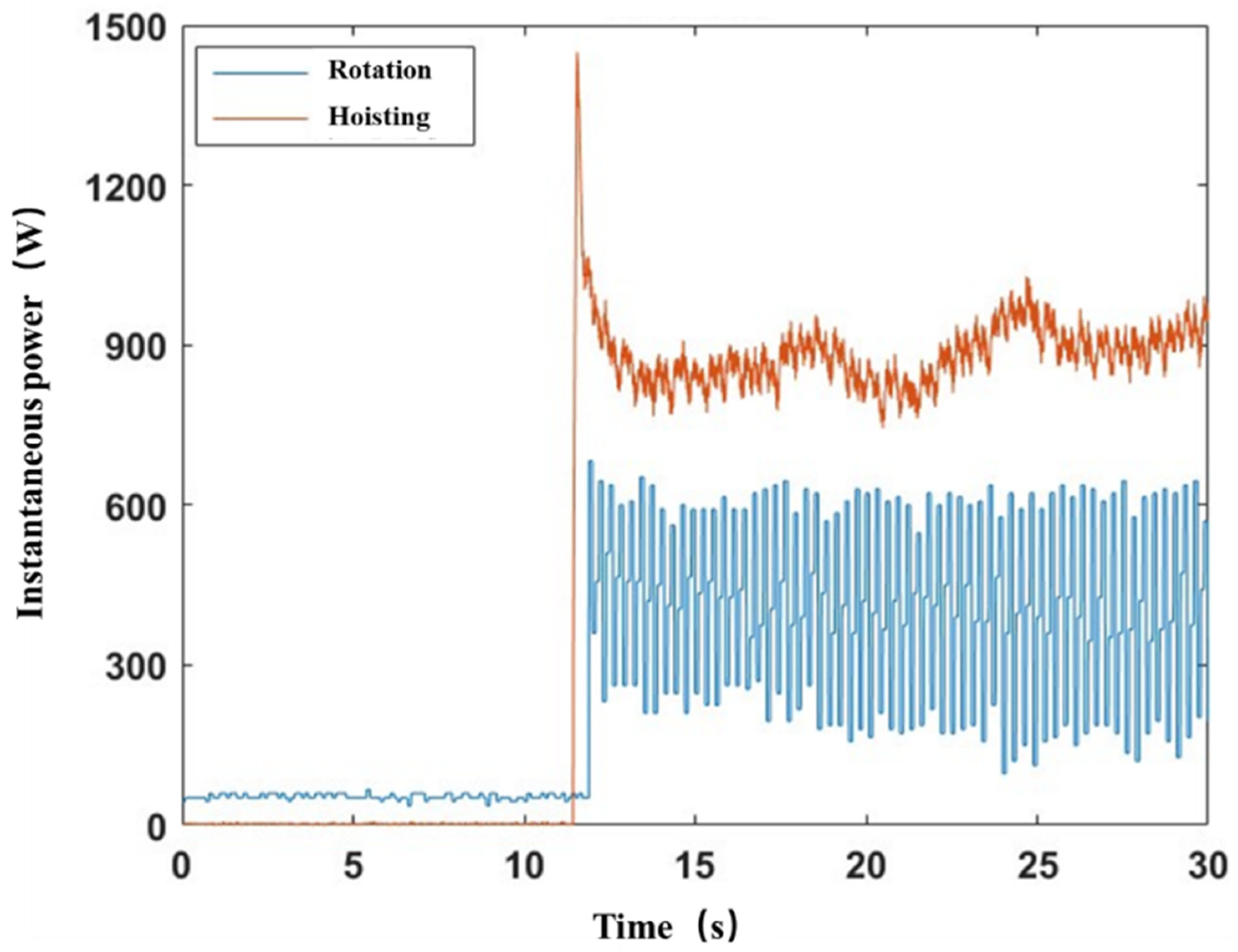
Drill bits were divided into six groups. One group was the no-load control group, which was operated under the no-load condition without drilling the samples. The other five groups were drilled at the ROP of 2.6 m/h, 2.3 m/h, 2.0 m/h, 1.7 m/h, and 1.4 m/h, respectively, and the rotary speed ranged from 300 to 1000 rpm. The instantaneous powers of the two motors were recorded during drilling.

Power calibration is required to calculate the average value of the instantaneous power results obtained under no-load operation. As shown in Figure 14, the no-load fluctuation of the rotation motor is significant, the instantaneous average power is 400 W, and the hosting motor has an average power of 855 W.

In addition to energy consumption in the hole, mechanical consumption also occurs during drilling. The results are different when the ROP changes and RPM remains unchanged, as shown in Figure 15.

From the power perspective, the best rotary speed is between 700~1000 rpm, and the best ROP is between 2.0~2.6 m/h for the rock samples and drill bits used in the experiment.

In this chapter, four drilling modes are evaluated by experiments. The control of WOB under constant-pressure drilling mode is affected by drilling rules, and the control error of WOB under appropriate drilling rules is small. The maximum error of ROP control under constant-speed drilling mode is no more than 1.4%. Constant-torque drilling mode cannot achieve torque control, and it is prone to sticking, so it is not suitable for drilling in this system, but it can meet some specific innovative experiments. In the constant-power drilling mode, the performance was achieved by drilling at a given power within the appropriate range for a given drilling schedule. Therefore, the constant-speed drilling mode was selected as the main drilling mode, and was the best among the four drilling modes. Subsequently, a power-based optimization experiment was conducted for this drilling mode, and encouraging results were obtained. For the cement sample used in the experiment, the optimal rotary speed was in the range of 700~1000 rpm, and the optimal ROP was in the range of 2.0~2.6 m/h.

6. Conclusions and Discussion

In this study, the 2-DOF dynamics of the core drilling are modeled in detail, where the connections between drill bit and power head are treated as rotational springs. Then, A purely electric drive electronic control system using PLC technology and a servo motor servo system was used to develop a diamond-impregnated core drilling system that can be used to realize automatic drilling. Using the dynamic model of drill string and linearization control technology, a control system was developed to realize the process control of the drilling process. Then, four drilling modes were developed for the system: the performance of the different modes was verified experimentally, and the constant-speed mode was recommended as the conventional drilling mode. Finally, A power optimization drilling experiment based on motor performance was conducted, and a reasonable power optimization drilling procedure is provided herein. In the experiment, a φ46 diamond-impregnated drill bit was used to drill the rock samples, and a vast amount of data were obtained by changing the rotary speed and ROP. The power optimization results show that the optimal rotary speed was in the range of 700~1000 rpm, and the optimal ROP was in the range of 2.0~2.6 m/h. Compared with the previous laboratory automatic drill system, this study redesigned and developed the automatic electric drive drilling system with higher WOB and rotation speed for the characteristic of core drilling. Overall, this study provides a practical solution for electrically driven core drilling system in the laboratory, from complete setup to control design and validation.

However, the drilling system was in the early stages of development; only concrete was used instead of rock samples for drilling, although we used the same bit diameter as in the actual project. Moreover, this system has not been adequately tested on hard rocks. In addition, we used only a simple optimization algorithm to achieve optimization with high time complexity. We provide interfaces for further optimization; after optimization, we aim to compute the fast responses in real time to achieve intelligent drilling. Another problem is that because of the shallow drilling depth, the change in pump pressure is not noticeable; therefore, the system feedback cannot be completed according to the change in pump pressure, which is what we need to optimize. In future, experiments will be conducted to validate the drilling performance of the system using different rock types, and a machine learning algorithm will be applied to attain optimization while drilling and achieve formation identification.