Performance Evaluation of Different Decision Fusion Approaches for Image Classification

Abstract

Image classification is one of the major data mining tasks in smart city applications. However, deploying classification models that have good generalization accuracy is highly crucial for reliable decision-making in such applications. One of the ways to achieve good generalization accuracy is through the use of multiple classifiers and the fusion of their decisions. This approach is known as “decision fusion”. The requirement for achieving good results with decision fusion is that there should be dissimilarity between the outputs of the classifiers. This paper proposes and evaluates two ways of attaining the aforementioned dissimilarity. One is using dissimilar classifiers with different architectures, and the other is using similar classifiers with similar architectures but trained with different batch sizes. The paper also compares a number of decision fusion strategies.

1. Introduction

By 2050, 68 percent of the world’s population would be living in cities. As a result, managing existing infrastructure and resources to provide sustainable urban living conditions for the urban population’s growing demands is becoming more difficult [1]. Furthermore, advances in big data, the Internet of Things (IoT), information and communication technologies (ICT), data mining, and machine learning are paving the way for the transformation of cities into smart cities. The incorporation of these technologies into various urban sectors allows city administrators to gain access to the information they need for improved planning and better resource management [2]. A number of cities around the world have already begun to implement these technologies in order to improve the well-being, health, mobility, security, and comfort of their residents [3]. However, in order to realize the dream of smart cities and the technological advancements in other domains, we need to have machine learning/deep learning models that yield highly accurate results for facilitating accurate decision-making. One of the ways to fulfill this requirement is through the utilization of decision fusion in such applications. “Decision fusion” is the fusion of decisions from multiple classifiers [4].

The main data mining task in smart city applications is classification. Classification is the method of assigning different classes to the data instances based on their features. This paper focuses on decision fusion for image classification. The prime motive of the paper is to utilize decision fusion for improving classification accuracy, which is important for reliable decision-making in smart city applications. More precisely, the contribution of this work is as follows:

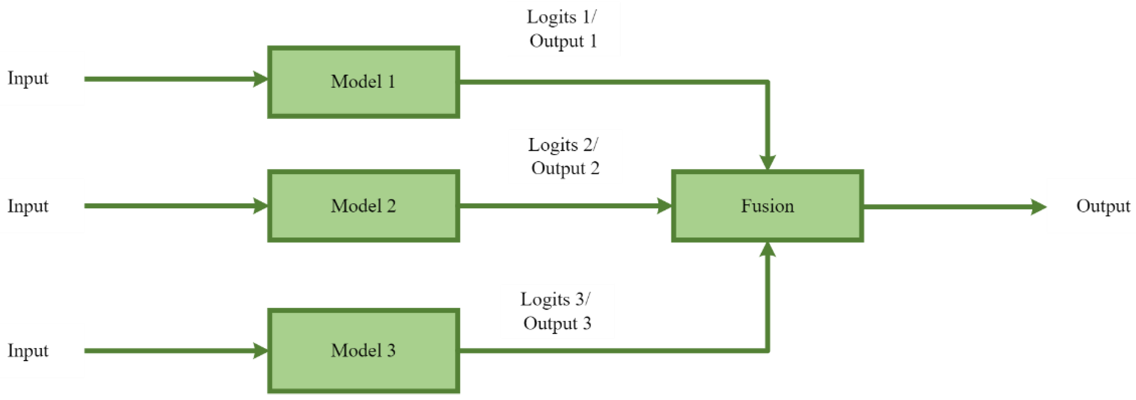
• The paper proposes and evaluates two approaches for attaining the dissimilarity between the outputs of the classifiers, which is crucial for getting good performance using decision fusion. One is using dissimilar classifiers with different architectures, and the other is using similar classifiers with similar architectures but trained with different batch-sizes.
• The paper compares the different decision fusion strategies for both of the aforementioned approaches.
• The paper investigates the correlation between the number of dissimilar outputs between the classifiers and the performance increase due to the decision fusion of these classifiers.

The remainder of the paper is structured as follows; Section 2 presents the literature review, citing the importance of image classification in smart city applications and the need for accurate classification in such applications. Section 3 discusses the preliminaries of the study. Section 4 discusses the proposed model. The section also presents the different decision-fusion strategies. Section 5 presents the experimental results and their analysis. Finally, Section 6 presents the concluding remarks.

2. Literature Review

Due to the growth of cities, new issues such as scarcity of resources, parking slot allotment, pollution, traffic congestion, etc. arise. As a result, designing strategies for meeting the current and future demands of the city is a top concern for all. Many projects, ranging from city councils and enterprises to research laboratories, are springing up around the world to facilitate quality living in cities. The smart city notion arose a few years ago as a collection of ideas about how advancements in areas such as ICT, IoT, big data, data mining, and machine learning could improve the working of cities. A number of cities around the world have already begun to implement these ideas. Smart city initiatives are classified into the following domains: smart healthcare [5,6], smart transportation [7,8], smart grid [9,10], smart buildings [3], smart manufacturing [3], smart economy [3], smart governance [3], and smart energy [3]. The following presents examples of the smart city domains and the importance of image classification in these domains.

Intelligent, energy-efficient, wirelessly networked medical equipment forms the core of smart healthcare [5]. The smart healthcare has been recognized as a panacea for easing the burden on healthcare systems. In addition, image classification is one of the major data mining tasks in smart healthcare. It is performed in a range of smart healthcare use cases such as disease diagnosis, disease risk prediction, better patient monitoring, and elderly fall detection. Examples of the studies that have performed image classification in smart healthcare use-cases are [11,12,13,14]. Further, in making reliable and justified decisions in smart healthcare, accurate image classification is highly important.

The sensors used to measure the traffic conditions are not effective enough in providing a comprehensive and accurate state of the traffic [7,8]. Several supplementary sources of data, such as probe vehicles, mobile phones, GPS, and cameras, are being used to enhance the information provided by the traffic sensors. As a result, image classification is crucial for the analytics of such data. Further, image classification is being performed in smart transportation use cases for facilitating applications such as position estimation, traffic monitoring, traffic demand forecasting, crash analysis and prevention, and advanced driver assistance. Examples of the studies that have performed image classification in smart transportation use-cases are [15,16,17,18]. All these applications are possible only if the image classification models generate accurate results. Hence, it is highly crucial to deploy classification models that have good generalization abilities.

The electrical grid serves as a hub for relaying electricity from power plants to homes and industries [9]. The integration of ICT transforms the electric grid into a smart grid, and the vision of the smart grid is to provide reliable and efficient electricity supply to consumers [10]. As a result, image classification is one of the major data mining tasks in smart grid applications. Further, image classification is being performed in smart grid use cases for facilitating applications such as energy demand forecasting, fault diagnosis, and anomaly detection. These applications are critical for the reliable and stable operation of the power grids. Examples of the studies that have performed image classification in smart grid use-cases are [19,20,21]. In order to realize the vision of the smart grid to its full potential, it is crucial that the models used for image classification generate accurate results.

Additionally, given the dire need for accurate image classification in smart city applications, it is crucial to use classification models that have good generalization accuracy. Motivated to resolve this challenge, this work proposes the idea of using decision fusion for image classification in smart city applications for better performance. A number of research studies have already utilized decision fusion in various smart city applications. These include medical image classification [22], covid detection [23], heart disease prediction [24], fault diagnosis [25], identification of osteoporosis [26], Alzheimer disease diagnosis [27], speech recognition [28], electric load forecasting [29], energy forecasting [30], anomaly detection [31], robotic arm control [32], soil temperature estimation [33], crowd counting [34], and pedestrian detection [35]. Some other works have fused the decisions of the classifier by inputting different modalities into the same classifier. Examples of such studies are [36,37,38]. The difference between this work and the existing works is that this work proposes and compares two ways of attaining dissimilarity between the outputs of classifiers in order to get better performance with decision fusion. One is using dissimilar classifiers with different architectures, and the other is using similar classifiers with similar architectures but trained using different batch sizes. Moreover, the paper compares different decision fusion approaches. The experiments have been conducted on Cifar-10, which is a benchmark dataset for image classification. The findings of the study can be applied to any image classification task.

3. Technical Background

This section discusses the architectures of VGG16, VGG19, and Resnet56.

Table 1. VGG16 Architecture.

Conv2d(3, 64, kernel_size = (3, 3))

Conv2d(64, 64, kernel_size = (3, 3))

MaxPool2d

Conv2d(64, 128, kernel_size = (3, 3))

Conv2d(128, 128, kernel_size = (3, 3))

MaxPool2d

Conv2d(128, 256, kernel_size = (3, 3))

Conv2d(256, 256, kernel_size = (3, 3))

Conv2d(256, 256, kernel_size = (3, 3))

MaxPool2d

Conv2d(256, 512, kernel_size = (3, 3))

Conv2d(512, 512, kernel_size = (3, 3))

Conv2d(512, 512, kernel_size = (3, 3))

MaxPool2d

Conv2d(512, 512, kernel_size = (3, 3))

Conv2d(512, 512, kernel_size = (3, 3))

Conv2d(512, 512, kernel_size = (3, 3))

MaxPool2d

Linear(512, 512)

Linear(512, 10)

Softmax

presents the architecture of VGG16. It consists of thirteen convolutional layers, two fully connected layers, and a soft max layer at the end. The convolutional layers carry out feature extraction, and the fully connected layers, along with the soft max layer, perform classification. Every convolutional layer in the table is represented as; Conv2d(in-channels, out-channels, kernel_size = ( , )), where in-channels denotes the number of input channels, out-channels denotes the number of output channels, and kernel-size is the size of the kernel. The fully connected layers are represented as linear (in-features and out-features), where in-features represent the number of input features and out-features represent the number of output features. MaxPool2d applies the max pool operation for downsampling the input. Each convolutional layer is followed by a batch-normalization layer and a Rectified Linear Unit (ReLU) activation function. The batch-normalization process accelerates the training process and improves its stability. Further, the ReLU is a non-linear activation function given as: $f\left(x\right)=\max \left(0,x\right)$.

Table 2. VGG19 Architecture.

Conv2d(3, 64, kernel_size = (3, 3))

Conv2d(64, 64, kernel_size = (3, 3))

MaxPool2d

Conv2d(64, 128, kernel_size = (3, 3))

Conv2d(128, 128, kernel_size = (3, 3))

MaxPool2d

Conv2d(128, 256, kernel_size = (3, 3))

MaxPool2d

Conv2d(256, 256, kernel_size = (3, 3))

Conv2d(256, 256, kernel_size = (3, 3))

Conv2d(256, 256, kernel_size = (3, 3))

MaxPool2d

Conv2d(256, 512, kernel_size = (3, 3))

Conv2d(512, 512, kernel_size = (3, 3))

Conv2d(512, 512, kernel_size = (3, 3))

Conv2d(512, 512, kernel_size = (3, 3))

MaxPool2d

Conv2d(512, 512, kernel_size = (3, 3))

Conv2d(512, 512, kernel_size = (3, 3))

Conv2d(512, 512, kernel_size = (3, 3))

Conv2d(512, 512, kernel_size = (3, 3))

MaxPool2d

Linear(512, 512)

Linear(512, 10)

Softmax

presents the architecture of VGG19. It consists of sixteen convolutional layers, two fully connected layers, and a softmax layer at the end. Each convolutional layer is followed by a batch-normalization layer and ReLU activation function.

Table 3. Resnet56 Architecture.

Conv2d(3, 16, kernel_size = (3, 3))	×1
Conv2d(16, 16, kernel_size = (3, 3))	×9
Conv2d(16, 16, kernel_size = (3, 3))
Conv2d(16, 32, kernel_size = (3, 3))	×1
Conv2d(32, 32, kernel_size = (3, 3))
Conv2d(16, 32, kernel_size = (3, 3))
Conv2d(32, 32, kernel_size = (3, 3))	×8
Conv2d(32, 32, kernel_size = (3, 3))
Conv2d(32, 64, kernel_size = (3, 3))	×1
Conv2d(64, 64, kernel_size = (3, 3))
Conv2d(32, 64, kernel_size = (3, 3))
Conv2d(64, 64, kernel_size = (3, 3))	×8
Conv2d(64, 64, kernel_size = (3, 3))
Linear(64, 10)	×1
Softmax

presents the architecture of ResNet56. Each convolutional layer is followed by a batch-normalization layer.

4. Proposed Model

This paper proposes two ways of achieving dissimilarity between the outputs of classifiers, which is a must for achieving better performance results using decision fusion. The generalized model for the decision fusion approach is shown in Figure 1.

Three models, model 1, model 2, and model 3, are trained on the training dataset, and the data from the test dataset is fed as input to the three models. Then the logits/outputs from these models are fused to produce the output. The fusion strategies that have been used are illustrated in Figure 2.

These include; ‘majorityvoting’, ‘maximum’, ‘sum’, ‘product’ and ‘minimum’. Suppose $l_i\left(x\right)$ and $O_i\left(x\right)$ represent the logits and the output of the $i\mathrm{th}$ classifier, respectively, for the input vector $x$. In case of ‘majorityvoting’, the class with maximum number of votes is chosen as the output class. The output in the case of majority voting is calculated using Equation (1);

$$Output\left(x\right)=argma{x}_{j=1}^n{\sum }_{i=1}^3{O}_i\left(x\right)$$

(1)

where $n$ is the number of classes. For Cifar-10$, n=10$.

‘Maximum’ fusion strategy compares logit 1, logit 2 and logit 3 and chooses the maximum logit for each class. The output in case of ‘Maximum’ fusion is calculated using Equation (2);

$$Output\left(x\right)=argma{x}_{j=1}^{n}Ma{x}_{i=1}^3{l}_i\left(x\right)$$

(2)

In the ‘Sum’ fusion strategy, the sum of logit 1, logit 2; and logit 3 is calculated for each class, and then the class with the maximum logit value is chosen as the output class. The output in case of ‘Sum’ fusion is calculated using Equation (3);

$$Output\left(x\right)=argma{x}_{j=1}^n{\sum }_{i=1}^3{l}_i\left(x\right)$$

(3)

The ‘Product’ fusion strategy computes the product of logit 1, logit 2 and logit 3 for each class, and then the class with the maximum logit value is chosen as the output class. The output in the case of ‘Product’ fusion is calculated using Equation (4);

$$Output\left(x\right)=argma{x}_{j=1}^n{\prod }_{i=1}^3{l}_i\left(x\right)$$

(4)

In the case of ‘Minimum’ fusion strategy, the minimum value among logit 1, logit 2, and logit 3 from each class is chosen, and then the class with the maximum logit value is chosen as the output class. The output in case of ‘Minimum’ fusion is calculated using Equation (5);

$$Output\left(x\right)=argma{x}_{j=1}^{n}Mi{n}_{i=1}^3{l}_i\left(x\right)$$

(5)

The requirement for decision fusion to produce good results is that models 1, 2, and 3 should make different predictions on a number of test samples. That is, there should be a number of input samples for which; $O_i\ne O_j where i=1, 2, 3;j=1, 2, 3 ;and i\ne j$. This paper satisfies the above requirement in two ways; (1) three different model architectures are used, (2) models with the same architectures but different batch-sizes are used. The models that have been chosen are; VGG16, VGG19, and Resnet56. The batch sizes that have been used are 128, 512, and 1024. This is illustrated by Figure 3 and Figure 4.

5. Results and Analysis

The experiments were conducted on a Tesla T4 GPU using Pytorch. Three models, namely, VGG16, VGG19, and ResNet56, were trained on the Cifar10 dataset, which consists of images of ten different objects. The dataset comprises 50,000 images for training and 10,000 for testing. The hyper-parameters used for training the models are given in

Table 4. Hyper-parameters for the models.

Hyper-Parameters	Value
Epochs	300
Learning Rate	0.1
Learning Rate Decay	0.1
Optimizer	SGD
Momentum	0.9
Weight Decay	0.0005
Batch-Sizes	128, 512, 1024
Loss-function	Cross-Entropy loss

. The models were trained with three different batch sizes: 128, 512, and 1024. VGG16 models with three different batch sizes are represented as; VGG16_128; VGG16_512, and VGG16_1024. VGG19 models with three different batch sizes are represented as VGG19_128, VGG19_512; and VGG19_1024. Similarly, ResNet56 with three different batch sizes is represented as; ResNet56_128; ResNet56_512; and ResNet56_1024.

Figure 5 presents the accuracies of the above-mentioned models. ResNet56_128 outperforms the other models and gives an accuracy of 94.14%. The ResNet56_1024 shows poor performance among all the models and gives an accuracy of 92.97%. Among VGG16_128, VGG16_512, and VGG16_1024, VGG16_128 outperforms the other two and gives an accuracy of 94%. Among VGG19_128, VGG19_512, and VGG19_1024, VGG19_128 outperforms the other two and gives an accuracy of 93.9%. Similarly, among ResNet56_128, ResNet56_512, and ResNet56_1024, ResNet56_128 outperforms the other two and gives an accuracy of 94.14%.

Figure 6a–c present the number of samples with dissimilar outputs in the case of similar models with different batch-sizes. Figure 6a presents the number of samples with dissimilar outputs in the cases of VGG16_128 and VGG16_512, VGG16_512 and VGG16_1024, and VGG16_128 and VGG16_1024. There are 594 samples with dissimilar outputs between VGG16_128 and VGG16_512, 614 samples with dissimilar outputs between VGG16_512 and VGG16_1024, and 646 samples with dissimilar outputs between VGG16_128 and VGG16_1024. Figure 6b presents the number of samples with dissimilar outputs in the cases of VGG19_128 and VGG19_512, VGG19_512 and VGG19_1024, and VGG19_128 and VGG19_1024. There are 596 samples with dissimilar outputs between VGG19_128 and VGG19_512, 598 samples with dissimilar outputs between VGG16_512 and VGG16_1024, and 639 samples with dissimilar outputs between VGG16_128 and VGG16_1024. Figure 6c presents the number of samples with dissimilar outputs in the cases of ResNet56_128 and ResNet56_512, ResNet56_512 and ResNet56_1024, and ResNet56_128 and ResNet56_1024. There are 577 samples with dissimilar outputs between ResNet56_128 and ResNet56_512, 661 samples with dissimilar outputs between ResNet56_512 and ResNet56_1024, and 651 samples with dissimilar outputs between ResNet56_128 and ResNet56_1024.

Figure 6d–f present the number of samples with dissimilar outputs in the case of dissimilar models. Figure 6d presents the number of samples with dissimilar outputs in cases of VGG16_128 and VGG19_128, VGG19_128 and ResNet56_128, and VGG16_128 and ResNet56_128. There are 582 samples with dissimilar outputs between VGG16_128 and VGG19_128, 645 samples with dissimilar outputs between VGG19_128 and ResNet56_128, and 625 samples with dissimilar outputs between VGG16_128 and ResNet56_128. Figure 6e presents the number of samples with dissimilar outputs in the cases of VGG16_512 and VGG19_512, VGG19_512 and ResNet56_512, and VGG16_512 and ResNet56_512. There are 583 samples with dissimilar outputs between VGG16_128 and VGG19_128, 661 samples with dissimilar outputs between VGG19_512 and ResNet56_512, and 671 samples with dissimilar outputs between VGG16_512 and ResNet56_512. Figure 6f presents the number of samples with dissimilar outputs in the case of VGG16_1024 and VGG19_1024, VGG19_1024 and ResNet56_1024, and VGG16_1024 and ResNet56_1024. There are 573 samples with dissimilar outputs between VGG16_128 and VGG19_128, 727 samples with dissimilar outputs between VGG19_1024 and ResNet56_1024, and 728 samples with dissimilar outputs between VGG16_1024 and ResNet56_1024.

As already discussed, the requirement for the decision-fusion to produce better results is that the models that are to be fused should make dissimilar predictions on a number of test samples. In addition, from the above graphs, it is clear that there is a dissimilarity between the predictions of the aforementioned models. Figure 7a–c present the accuracy of the fused models in the case of fusion of similar models with different batch-sizes using different fusion strategies. Figure 7a presents the accuracy of the fused model obtained by the fusion of VGG16_128, VGG16_512, and VGG16_1024 using fusion strategies; ‘majority-voting’, ‘maximum’, ‘sum’, ‘product’ and ‘minimum’. It is clear from the graph that the fusion obtained by summing the logits of the three models for all the classes and then choosing the class with the maximum logit value as the output class (‘Sum’ fusion) outperforms all the other fusion strategies discussed in this paper. Figure 7b presents the accuracy of the fused model obtained by the fusion of VGG19_128, VGG19_512, and VGG19_1024 using the aforementioned fusion strategies. The graph shows that the fusion obtained by taking the maximum logit value among the logit values of the three models for all the classes and then choosing the class with the maximum logit value as the output class (‘Maximum’ fusion) outperforms all the other fusion strategies. The accuracy given by the ‘sum’ fusion technique is slightly smaller than the accuracy given by the ‘maximum’ fusion technique. Figure 7c presents the accuracy of the fused model obtained by the fusion of ResNet56_128, ResNet56_512, and ResNet56_1024 using the aforementioned fusion strategies. The graph shows that the ‘Sum’ fusion technique outperforms all the other fusion techniques.

Figure 8a–c present the accuracy of the fused models in the case of the fusion of dissimilar models using different fusion strategies. Figure 8a presents the accuracy of the fused model obtained by the fusion of VGG16_128 and VGG19_128 with ResNet56_128 using different fusion strategies. It is clear from the graph that the fusion obtained by ‘Sum’ fusion technique performs better than all the other fusion strategies. Figure 8b presents the accuracy of the fused model obtained by the fusion of VGG16_512, VGG19_512, and ResNet56_512 using different fusion strategies. It is clear from the graph that the fusion obtained by ‘Sum’ fusion technique performs better than all the other fusion strategies. Figure 8c presents the accuracy of the fused model obtained by the fusion of VGG16_1024, VGG19_1024, and ResNet56_10124 using the aforementioned fusion strategies. The graph shows that the ‘Sum’ fusion technique outperforms all the other fusion techniques.

Figure 9a–e present the accuracy of the fused models with different model combinations for each fusion strategy. These model combinations include; (a) combining similar models with different batch sizes. These include the following combinations; VGG16_128 + VGG16_512, + VGG16_1024, VGG19_128 + VGG19_512 + VGG19_1024, and ResNet56_128 + ResNet56_512 + ResNet56_1024, (b) Combining dissimilar models. These include the following combinations; VGG16_128 + VGG19_128 + ResNet56_128, VGG16_512+ VGG19_512 + ResNet56_512, and VGG16_1024 + VGG19_1024 + ResNet56_1024. Figure 9a presents the accuracy of different model combinations using ‘Maximum Voting’ fusion. It is clear from the graph that the fusion obtained by the following model combination: VGG16_128 + VGG19_128 + ResNet56_128 performs better than all the other model combinations using Majority Voting. Figure 9b presents the accuracy of different model combinations using ‘Maximum’ fusion. It is clear from the graph that the fusion obtained by the following model combination: VGG16_128 + VGG19_128 + ResNet56_128 performs better than all the other model combinations using ‘maximum’ fusion. Figure 9c presents the accuracy of different model combinations using ‘Sum’ fusion. It is clear from the graph that the fusion obtained by the following model combination: VGG16_128 + VGG19_128 + ResNet56_128 performs better than all the other model combinations using ‘Sum’ fusion. Figure 9d presents the accuracy of different model combinations using ‘Product’ fusion. It is clear from the graph that the fusion obtained by the following model combination: VGG16_128 + VGG19_128 + ResNet56_128 performs better than all the other model combinations using ‘product’ fusion. Figure 9e presents the accuracy of different model combinations using ‘minimum’ fusion. It is clear from the graph that the fusion obtained by the following model combination: VGG16_128 + VGG19_128 + ResNet56_128 performs better than all the other model combinations using ‘minimum’ fusion.

From the above discussion, we can summarize that among the different model combinations, VGG16_128 + VGG19_128 + ResNet56_128 performs better than the others, and among the different fusion strategies, ‘Sum’ produces better results than the other fusion strategies.

Table 5. Comparison with the baseline models.

Model	Accuracy (%)
VGG16_128	94
VGG19_128	93.9
ResNet56_128	94.14
VGG16_128 + VGG19_128 + ResNet56_128	95.46

presents the comparison of VGG16_128 + VGG19_128 + ResNet56_128 with the baseline models.

In considering the individual models in the aforementioned combination, VGG16_128 gives an accuracy of 94%, VGG19_128 gives an accuracy of 93.9%, and ResNet56_128 gives an accuracy of 94.14%. The best of the three is ResNet56_128 with an accuracy of 94.14%. The decision fusion with the model combination VGG16_128 + VGG19_128 + ResNet56_128 gives an accuracy of 95.46%, which means an improvement of 1.32% over the best individual model in the combination. However, if we look at the number of dissimilar cases, the number of dissimilar cases is highest in the case of VGG16_1024 + VGG19_1024 + ResNet56_1024, which means that accuracy increase does not correlate well with the number of dissimilar cases. Hence, investigating the dissimilarity measure that correlates well with the accuracy increase is crucial.

6. Conclusions

The paper proposed and evaluated two approaches for attaining dissimilar outputs between the classifiers, which is a pre-requisite for achieving better results with decision fusion. These two approaches are; decision-fusion of dissimilar classifiers with different architectures, and decision-fusion of classifiers with similar architectures but trained using different batch-sizes. The VGG16, VGG19, and ResNet56 were trained on the Cifar-10 dataset with three different batch sizes: 128, 512, and 1024, and the decisions of the models were fused. The model combinations that were obtained are: VGG16_128 + VGG19_128 + ResNet56_128, VGG16_512 + VGG19_512 + ResNet56_512, VGG16_1024 + VGG19_1024 + ResNet56_1024, VGG16_128 + VGG16_512 + VGG16_1024, VGG19_128 + VGG19_512 + VGG19_1024, and ResNet56_128 + ResNet56_512 + ResNet56_1024. These models were fused with a number of fusion strategies. These included ‘Majority-Voting’, ‘Maximum’, ‘Sum’, ‘Product’ and ‘Minimum’. Among the fusion strategies, the ‘Sum’ strategy outperformed the others. In addition, among the different model combinations, VGG16_128 + VGG19_128 + ResNet56_128 performed better. For every model combination, the number of samples with dissimilar outputs was calculated. However, the number of dissimilar outputs did not correlate well with the accuracy increase because of decision fusion. The future work would be to investigate the dissimilarity measure that correlates well with the accuracy increase. Furthermore, the utilization of decision fusion for getting better classification accuracy is computationally expensive, and there might be scenarios in smart city applications where the resources are constrained in terms of computation and storage. Hence, investigating the computationally efficient methods for achieving higher classification accuracy in such scenarios is crucial.

References

1. Camero, A.; Alba, E. Smart City and information technology: A review. Cities 2019, 93, 84–94. [Google Scholar] [CrossRef]
2. Anthopoulos, L.G. Understanding the smart city domain: A literature review. In Transforming City Governments for Successful Smart Cities; Springer: Cham, Switzerland, 2015; pp. 9–21. [Google Scholar]
3. Gaur, A.; Scotney, B.; Parr, G.; McClean, S. Smart city architecture and its applications based on IoT. Procedia Comput. Sci. 2015, 52, 1089–1094. [Google Scholar] [CrossRef]
4. Krishnamurthi, R.; Kumar, A.; Gopinathan, D.; Nayyar, A.; Qureshi, B. An overview of IoT sensor data processing, fusion, and analysis techniques. Sensors 2020, 20, 6076. [Google Scholar] [CrossRef] [PubMed]
5. Ghazal, T.M.; Hasan, M.K.; Alshurideh, M.T.; Alzoubi, H.M.; Ahmad, M.; Akbar, S.S.; Al Kurdi, B.; Akour, I.A. IoT for smart cities: Machine learning approaches in smart healthcare—A review. Future Internet 2021, 13, 218. [Google Scholar] [CrossRef]
6. Kumar, A.; Krishnamurthi, R.; Nayyar, A.; Sharma, K.; Grover, V.; Hossain, E. A novel smart healthcare design, simulation, and implementation using healthcare 4.0 processes. IEEE Access 2020, 8, 118433–118471. [Google Scholar] [CrossRef]
7. Zantalis, F.; Koulouras, G.; Karabetsos, S.; Kandris, D. A review of machine learning and IoT in smart transportation. Future Internet 2019, 11, 94. [Google Scholar] [CrossRef] [Green Version]
8. Kelley, S.B.; Lane, B.W.; Stanley, B.W.; Kane, K.; Nielsen, E.; Strachan, S. Smart transportation for all? A typology of recent U.S. smart transportation projects in midsized cities. Ann. Assoc. Am. Geogr. 2019, 110, 547–558. [Google Scholar] [CrossRef]
9. Dileep, G. A survey on smart grid technologies and applications. Renew. Energy 2019, 146, 2589–2625. [Google Scholar] [CrossRef]
10. Neffati, O.S.; Sengan, S.; Thangavelu, K.D.; Kumar, S.D.; Setiawan, R.; Elangovan, M.; Mani, D.; Velayutham, P. Migrating from traditional grid to smart grid in smart cities promoted in developing country. Sustain. Energy Technol. Assess. 2021, 45, 101125. [Google Scholar] [CrossRef]
11. Dutta, A.; Batabyal, T.; Basu, M.; Acton, S.T. An efficient convolutional neural network for coronary heart disease prediction. Expert Syst. Appl. 2020, 159, 113408. [Google Scholar] [CrossRef]
12. Ambekar, S.; Phalnikar, R. Disease risk prediction by using convolutional neural network. In Proceedings of the 2018 Fourth International Conference on Computing Communication Control and Automation (ICCUBEA), Pune, India, 16–18 August 2018; pp. 1–5. [Google Scholar]
13. Gul, M.A.; Yousaf, M.H.; Nawaz, S.; Rehman, Z.U.; Kim, H. Patient monitoring by abnormal human activity recognition based on CNN architecture. Electronics 2020, 9, 1993. [Google Scholar] [CrossRef]
14. Yu, M.; Gong, L.; Kollias, S. Computer vision based fall detection by a convolutional neural network. In Proceedings of the 19th ACM International Conference on Multimodal Interaction, Glasgow, UK, 13–17 November 2017; pp. 416–420. [Google Scholar]
15. Kurniawan, J.; Syahra, S.G.; Dewa, C.K.; Afiahayati. Traffic congestion detection: Learning from CCTV monitoring images using convolutional neural network. Procedia Comput. Sci. 2018, 144, 291–297. [Google Scholar] [CrossRef]
16. Zhu, Z.; Liang, D.; Zhang, S.; Huang, X.; Li, B.; Hu, S. Traffic-sign detection and classification in the wild. In Proceedings of the IEEE Conference on Computer Vision and Pattern Recognition, Las Vegas, NV, USA, 27–30 June 2016; pp. 2110–2118. [Google Scholar]
17. Ghosh, S.; Sunny, S.J.; Roney, R. Accident detection using convolutional neural networks. In Proceedings of the 2019 International Conference on Data Science and Communication (IconDSC), Bangalore, India, 1–2 March 2019; pp. 1–6. [Google Scholar]
18. Naik, D.B.; Lakshmi, G.S.; Sajja, V.R.; Venkatesulu, D.; Rao, J.N. Driver’s seat belt detection using CNN. Turk. J. Comput. Math. Educ. (TURCOMAT) 2021, 12, 776–785. [Google Scholar]
19. Mohammadpourfard, M.; Genc, I.; Lakshminarayana, S.; Konstantinou, C. Attack detection and localization in smart grid with image-based deep learning. In Proceedings of the 2021 IEEE International Conference on Communications, Control, and Computing Technologies for Smart Grids (SmartGridComm), Aachen, Germany, 25–28 October 2021; pp. 121–126. [Google Scholar] [CrossRef]
20. Agrawal, A.; Sethi, K.; Bera, P. IoT-Based Aggregate Smart Grid Energy Data Extraction using Image Recognition and Partial Homomorphic Encryption. In Proceedings of the 2021 IEEE International Conference on Advanced Networks and Telecommunications Systems (ANTS), Hyderabad, India, 13–16 December 2021; pp. 408–413. [Google Scholar]
21. Laroca, R.; Barroso, V.; Diniz, M.A.; Gonçalves, G.R.; Schwartz, W.; Menotti, D. Convolutional neural networks for automatic meter reading. J. Electron. Imaging 2019, 28, 013023. [Google Scholar] [CrossRef]
22. Ahn, E.; Kumar, A.; Feng, D.; Fulham, M.; Kim, J. Unsupervised feature learning with K-means and an ensemble of deep convolutional neural networks for medical image classification. arXiv 2019, arXiv:1906.03359. [Google Scholar]
23. Gifani, P.; Shalbaf, A.; Vafaeezadeh, M. Automated detection of COVID-19 using ensemble of transfer learning with deep convolutional neural network based on CT scans. Int. J. Comput. Assist. Radiol. Surg. 2020, 16, 115–123. [Google Scholar] [CrossRef]
24. Ali, F.; El-Sappagh, S.; Islam, S.R.; Kwak, D.; Ali, A.; Imran, M.; Kwak, K.-S. A smart healthcare monitoring system for heart disease prediction based on ensemble deep learning and feature fusion. Inf. Fusion 2020, 63, 208–222. [Google Scholar] [CrossRef]
25. Li, Y.; Song, Y.; Jia, L.; Gao, S.; Li, Q.; Qiu, M. Intelligent fault diagnosis by fusing domain adversarial training and maximum mean discrepancy via ensemble learning. IEEE Trans. Ind. Inform. 2020, 17, 2833–2841. [Google Scholar] [CrossRef]
26. Sukegawa, S.; Fujimura, A.; Taguchi, A.; Yamamoto, N.; Kitamura, A.; Goto, R.; Nakano, K.; Takabatake, K.; Kawai, H.; Nagatsuka, H.; et al. Identification of osteoporosis using ensemble deep learning model with panoramic radiographs and clinical covariates. Sci. Rep. 2022, 12, 6088. [Google Scholar] [CrossRef]
27. Ganaie, M.A.; Tanveer, M. Ensemble deep random vector functional link network using privileged information for Alzheimer’s disease diagnosis. IEEE/ACM Trans. Comput. Biol. Bioinform. 2022. [Google Scholar] [CrossRef]
28. Li, S.; Lu, X.; Sakai, S.; Mimura, M.; Kawahara, T. Semi-supervised ensemble DNN acoustic model training. In Proceedings of the 2017 IEEE International Conference on Acoustics, Speech and Signal Processing (ICASSP), New Orleans, LA, USA, 5–9 March 2017; pp. 5270–5274. [Google Scholar] [CrossRef]
29. Singla, P.; Duhan, M.; Saroha, S. An ensemble method to forecast 24-h ahead solar irradiance using wavelet decomposition and BiLSTM deep learning network. Earth Sci. Inform. 2021, 15, 291–306. [Google Scholar] [CrossRef] [PubMed]
30. Wen, L.; Xie, X.; Li, X.; Gao, L. A new ensemble convolutional neural network with diversity regularization for fault diagnosis. J. Manuf. Syst. 2020, 62, 964–971. [Google Scholar] [CrossRef]
31. Tsogbaatar, E.; Bhuyan, M.H.; Taenaka, Y.; Fall, D.; Gonchigsumlaa, K.; Elmroth, E.; Kadobayashi, Y. DeL-IoT: A deep ensemble learning approach to uncover anomalies in IoT. Internet Things 2021, 14, 100391. [Google Scholar] [CrossRef]
32. Zhang, J.; Zhang, W.; Song, R.; Ma, L.; Li, Y. Grasp for stacking via deep reinforcement learning. In Proceedings of the 2020 IEEE International Conference on Robotics and Automation (ICRA), Paris, France, 31 May–August 2020; pp. 2543–2549. [Google Scholar]
33. Kazemi, S.M.R.; Bidgoli, B.M.; Shamshirband, S.; Karimi, S.M.; Ghorbani, M.A.; Chau, K.-W.; Pour, R.K. Novel genetic-based negative correlation learning for estimating soil temperature. Eng. Appl. Comput. Fluid Mech. 2018, 12, 506–516. [Google Scholar] [CrossRef] [Green Version]
34. Shi, Z.; Zhang, L.; Liu, Y.; Cao, X.; Ye, Y.; Cheng, M.M.; Zheng, G. Crowd counting with deep negative correlation learning. In Proceedings of the IEEE Conference on Computer Vision and Pattern Recognition, Salt Lake City, UT, USA, 18–22 June 2018; pp. 5382–5390. [Google Scholar]
35. Yang, B.; Yan, J.; Lei, Z.; Li, S.Z. Convolutional channel features. In Proceedings of the IEEE International Conference on Computer Vision, Santiago, Chile, 7–13 December 2015; pp. 82–90. [Google Scholar]
36. Hu, B.; Li, Q.; Hall, G.B. A decision-level fusion approach to tree species classification from multi-source remotely sensed data. ISPRS Open J. Photogramm. Remote Sens. 2021, 1, 100002. [Google Scholar] [CrossRef]
37. Nadeem, M.W.; Goh, H.G.; Khan, M.A.; Hussain, M.; Mushtaq, M.F.; Ponnusamy, V.A. Fusion-based machine learning architecture for heart disease prediction. Comput. Mater. Contin. 2021, 67, 2481–2496. [Google Scholar] [CrossRef]
38. Teng, S.; Chen, G.; Liu, Z.; Cheng, L.; Sun, X. Multi-sensor and decision-level fusion-based structural damage detection using a one-dimensional convolutional neural network. Sensors 2021, 21, 3950. [Google Scholar] [CrossRef]
Figure 1. Decision fusion.
Applsci 13 01168 g001
Figure 2. Different Fusion Strategies.
Applsci 13 01168 g002
Figure 3. Fusion of dis-similar models.
Applsci 13 01168 g003
Figure 4. Fusion of similar models with different batch-sizes.
Applsci 13 01168 g004
Figure 5. Accuracy of different models.
Applsci 13 01168 g005
Figure 6. (af): Number of Samples with dissimilar outputs.
Applsci 13 01168 g006aApplsci 13 01168 g006bApplsci 13 01168 g006c
Figure 7. (ac): Accuracy using different fusion strategies in case of fusion of similar models with different batch-sizes.
Applsci 13 01168 g007
Figure 8. (ac): Accuracy using different fusion strategies in case of fusion of different models with same batch sizes.
Applsci 13 01168 g008aApplsci 13 01168 g008b
Figure 9. (ae): Accuracy with different model combinations for each fusion strategy.
Applsci 13 01168 g009aApplsci 13 01168 g009b