Article

A Study on Longitudinal Motion Scenario Design for Verification of Advanced Driver Assistance Systems and Autonomous Driving Systems

1
Department of Electrical Engineering, Hanyang University, Seoul 04763, Republic of Korea
2
Department of Electrical and Biomedical Engineering, Hanyang University, Seoul 04763, Republic of Korea
*
Author to whom correspondence should be addressed.
Appl. Sci. 2023, 13(2), 716; https://doi.org/10.3390/app13020716
Submission received: 29 October 2022 / Revised: 11 December 2022 / Accepted: 12 December 2022 / Published: 4 January 2023

Abstract

:
This paper proposes a test scenario design method that reflects the longitudinal characteristics of reality for effective verification of advanced driver assistance systems (ADAS) and autonomous driving systems (ADS). Since the target systems interact with the external environment differently from the existing vehicle control system, realistic and various verification scenarios are required for verification. The proposed method consists of a vehicle model for simulating the vehicle behavior and a driver model to actively respond to the driving environment. In particular, the driver model used a model predictive control (MPC) algorithm to reflect the characteristic of human drivers. The longitudinal driving characteristics of human drivers were derived through a large-scale driving database analysis and considered in the driver model. The proposed method was compared with an existing car-following model using computer simulations. It was confirmed that its longitudinal driving behavior is similar to that of human drivers and that various scenarios can be designed by changing the model parameters.

1. Introduction

A great deal of research has been carried out for decades to develop advanced driver assistance systems (ADAS) and autonomous driving systems (ADS) for drivers’ convenience and safety [1,2,3,4,5]. ADAS and ADS are closely related to safety, thus verification is required through various environments and scenarios. Recently, studies conducted using virtual vehicle and traffic simulation programs, such as IPG Carmaker and Carla, to improve the efficiency of ADAS and ADS design and verification are being actively conducted [6,7,8]. In addition, research on a vehicle in the loop (VIL) models that utilize the dynamic characteristics of real vehicles and interconnect with virtual environments is increasing [9,10,11,12]. Especially, ADAS and ADS operate organically with surrounding and external environments, hence the scenarios for verification in a simulation environment must consider various factors.
As scenario design methods for verification of ADAS and ADS, standards assessment-based, test matrix-based, malicious scenario-based, and traffic simulation-based methods are widely known [13,14,15,16,17,18,19,20,21]. First, there is a standards assessment-based method widely known as ISO and Euro NCAP [13,14]. The scenarios presented by these two organizations focus on the verification of autonomous emergency braking systems (AEBS), adaptive cruise control systems (ACCS), and lane support systems among ADAS. Although different models have different purposes in terms of vehicle safety assessment or establishing ADAS standards, they are similar in that they present minimum standards that ADAS must satisfy. As the scenarios provided by the two organizations are limited, these scenarios need to be expanded for drivers’ safety in various driving situations. A test matrix-based method can be used for designing various scenarios, which defines factors to be evaluated based on a large-scale database [15,20]. Many projects have suggested test scenarios using actual driving/accident data [15,16,17,18]. However, ADAS and ADS designed with known scenarios inevitably have lower reliability for scenarios that have not occurred ever. A malicious scenario-based method is one that defines scenarios near the limit of the mathematical models of the ego and surrounding vehicles [19,20,21]. This method can be verified in a short time because the verification is performed in the unstable regions of the ego and surrounding vehicles. However, when the system is very complex or designing a model of the system is not possible, it is difficult to design malicious scenarios. Last but not least, a traffic simulation-based method can be used to validate ADAS and ADS in a comprehensive environment. A traffic simulation is widely known as a method for macroscopic analysis of traffic volumes for road or signal system design [12,22,23]. This method is based on car-following models to simulate the traffic flow, and its application has recently been increasing for the verification of ADAS and ADS. Table 1 represents the list of widely known car-following models [24,25,26,27,28,29]. Each car-following model commonly uses the time constant τ to express the driver’s delay. In Table 1, v f , a f ,   R ,   R ˙ ,   R m i n , and V d represent the speed and acceleration of the ego vehicle, relative distance, speed and minimum relative distance with a leading vehicle, and the maximum speed of the ego vehicle, respectively. Other parameters ( C ,   C v ,   C s ,   C t , A , B , B ^ ) are configured to express various relative distances and speeds with a leading vehicle. Traffic simulation software is designed by improving the car-following models described in Table 1 [12,22,23]. Among the car-following models, only the Gipps model considers both acceleration and deceleration, which are the basic parameters governing the motion of the vehicle [28]. Therefore, it is not appropriate to use the remaining car-following models in the verification of ADAS and ADS, where the behavior of surrounding vehicles is important. As studies of ADAS and ADS became active in the 2000s, a large-scale naturalistic database was built to design the behavior of surrounding vehicles [18,30,31,32,33,34,35,36,37]. The 100-car naturalistic driving study (NDS) is a database of 3 million km of driving data from 241 drivers led by Virginia Tech [30]. Safety pilot model deployment (SPMD) is a database using roadside equipment and vehicle-mounted radar and vision to demonstrate the technology of connected vehicles in various environments and analyze driver acceptance of vehicle safety systems [35]. The High D dataset has collected driving data from more than 110,500 vehicles on highways in Germany and is being used in various ADAS and ADS studies [21,38]. Recently, using these large-scale driving databases, research on drivers’ driving characteristics and their application to car-following models is being actively conducted [29,39,40,41,42]. In [39], Bifulco defined the leading vehicle from the driving database and derived parameters of the Gipps model that follows it using artificial neural networks (ANNs). In [42], Przybyla deduced drivers’ characteristics through analysis of the driving database and applied them to the Newell model to analyze driving risk [42]. In [40], based on the NDS, Zheng derived the longitudinal acceleration and yaw angle of the following vehicle using reinforcement learning and a fuzzy algorithm. These methods are suitable for analyzing the traffic system by simulating the driving of the vehicle in a simulation environment like one facing an actual human driving. However, since it is difficult to design models for implementing malicious scenarios and control them, the traffic simulation-based method has limitations in ADAS and ADS verification.
Therefore, to overcome the limitations of the analyzed ADAS and ADS verification scenario design methods studied thus far, we propose a longitudinal motion scenario design method. In this method, the longitudinal driving characteristics of human drivers were reflected in the surrounding vehicles of the ego vehicle for more realistic scenario design in a simulation environment. First, a simplified vehicle dynamic model expresses the dynamic behavior of the vehicle, and a driver model imitates human driving by using model predictive control (MPC). With the vehicle and the driver model, the test vehicle can adapt to the surrounding environment and drive realistically, and various scenarios can be actively produced. Especially, to improve the consistency of the driver model, we determined the acceleration/deceleration standards for typical human drivers derived from a large-scale driving database analysis. Lastly, the proposed method was verified using computer simulations to confirm human driver imitations and their significance. The computer simulations assumed a driving situation on a straight-line road with a high road frictional coefficient. As the driving characteristics of human drivers vary depending on the driving situation, it was limited to the longitudinal acceleration/deceleration situation. The acceleration/deceleration and jerk, which are the longitudinal driving characteristics of human drivers, are derived in this situation. The characteristics of the sailing/braking start point are derived in this situation as well. To verify this and confirm consistency, the velocity, acceleration/deceleration, and jerk of the proposed method were compared with the acceleration/deceleration section of the randomly selected driver data. This study confirmed the possibility of simulating various drivers by changing the weights and constraints setting of the driver model. Through this, it is possible to create various longitudinal driving scenarios that overcome the shortcoming of the existing scenario design methods. In addition, if the constraints of the proposed driver model are set close to the limit situation, such as close distance to the surrounding vehicle or sudden stop, malicious scenarios can be easily designed with simple parameter changes.
This paper is organized as follows. Section 2 introduces a simplified vehicle model in more detail. Section 3 describes the error dynamics between the ego vehicle and surrounding vehicles and the design of an MPC-based driver model. Section 4 explains human driving characteristics derived from a large-scale database analysis. Section 5 shows the computer simulation results for the validation of the proposed method, and a conclusion is conducted in Section 6.

2. Simplified Vehicle Model

A simplified vehicle model for the longitudinal motion scenario design can simulate vehicle motion by inputting the required acceleration ( a x , d e s ), which is designed by the driver model proposed in Section 3. First, the simplified vehicle model assumes that the vehicle is traveling on flat ground, thus the relationship between the acceleration and velocity is shown in Equation (1) [43].
v ˙ x = a x
m a x = F x F r F a w . r . t   F r = N C r , 0 + C r , 1 v x + C r , 2 v x 2 F a = 0.5 C d ρ A v x 2
a x = a x ,   U i f   a x ,   d e s > a x , U a x ,   L e l s e   i f   a x , d e s < a L a x ,   d e s e l s e
To consider the dynamic characteristics of the vehicle, a longitudinal dynamic vehicle model is described in Equation (2). The vehicle acceleration is deduced by the longitudinal force ( F x ), rolling resistance ( F r ), and aerodynamic resistance ( F a ) of the vehicle. The rolling resistance ( F r ) is composed of the normal force of the vehicle ( N ), the constant coefficient ( C r , 0 ), and velocity coefficients ( C r , 1 ,   C r , 2 ). The aerodynamic resistance ( F a ) is composed of the aerodynamic drag coefficient ( C d ), the density of the air ( ρ ), and the area of the vehicle ( A ). The rolling resistance and the aerodynamic resistance are dependent on the vehicle velocity. The longitudinal force is constrained by the performance of the vehicle, which is related to the vehicle’s powertrain and braking system. For this reason, the longitudinal acceleration of the vehicle was constrained by an upper bound ( a x , U ) and lower bound ( a x , L ). Figure 1a describes the upper constraint of the longitudinal force that varies with the transmission gear ratio. For simplification, a simplified acceleration constraint, as shown in Figure 1b, is designed to consider dynamic characteristics of the vehicle in the longitudinal motion scenario design. It constrains the desired acceleration ( a x , d e s ) from the driver model to describe realistic vehicle motions. In other words, the actual vehicle is composed of complex dynamic systems, such as powertrain and hydraulic systems. However, in the case of this simplified vehicle model, it is used to simulate vehicle movement by considering acceleration and its related constraints. Acceleration and deceleration situations can occur depending on the sign of the longitudinal acceleration ( a x ), and the simplified vehicle model moves by causing a change in vehicle speed.

3. Longitudinal Driver Model

3.1. Error Dynamics for the Car-Following Model

To design a control input of the simplified vehicle model, Figure 2 a state-space equation is derived using the relative distance/velocity to the leading vehicle [43,44,45].
e x e v = x L , r v L x E G O , f v E G O c T G v E G O 0
d d t e x e v = 0 1 0 0 e x e v + c T G 1 a x + 0 1 a L x ˙ = A x + B u s . t   a m i n a x a m a x x m i n c t g v E G O   e x v L v E G P ,   m a x e v v L
In Equation (4), the desired relative distance ( c T G v E G O ) to the leading vehicle is determined using the constant time gap (CTG) policy to satisfy the string stability of a row of cars [44,45]. The distance error ( e x ) is designed using the desired relative distance and the difference between the rear of the leading vehicle ( x L , r ) and the front of the ego vehicle ( x E G O , f ). The velocity error ( e v ) is set as the difference between the velocity of the leading vehicle ( v L ) and the velocity of the ego vehicle ( v E G O ). The state equation constructed using the distance/velocity error is composed of the system matrices A , B , and the ego vehicle’s acceleration as input u . In order to simulate the movement of the ego vehicle for designing scenarios, a virtual target for deriving the distance/velocity error is required. For this reason, it is assumed that there is a virtual stopped vehicle ( v L ,   a L 0 ) in front of the vehicle model at a future stopping position or a virtual vehicle with constant velocity ( a L 0 ) to derive the distance/velocity error for simplification. The control input is constrained by the a m a x ,   a m i n that are defined by the characteristics of the vehicle and human drivers. In addition, the constraints of the distance/velocity error are defined to satisfy the CTG policy.

3.2. MPC-Based Driver Model Design

To design a driver model that considers human driving characteristics and various constraints using the simplified vehicle model, it is required that a controller should reflect future information and satisfy constraints. A model predictive control (MPC) algorithm is a well-known optimal controller design method to consider future states and constraints. The MPC algorithm is based on the discrete-time state-space model, and it calculates sub-optimal control inputs to minimize the cost function with various potential optimization methods [46]. The driver model of the proposed longitudinal motion scenario design method is designed by the MPC algorithm that minimizes the cost function ( J u ,   x 0 ) by satisfying the constraints in Equation (6).
J u , x 0 = x N T P x N + k = 0 N 1 x k T Q x k + u k T R u k s . t .   x k + 1 = A d x k + B d u k ,   k = 0 , ,   N 1 x k X ,   u k U ,   k = 0 ,   , N 1 x 0 = x 0 ,   P = P T > 0 ,   Q = Q T > 0 ,   R = R T > 0
The continuous time error dynamics model shown in Equation (4) is discretized by the Euler method, denoted by the discrete-time state-space model A d ,   B d to construct the MPC problem. X , U , and N are the constraints on the state, input, and prediction horizon, respectively. In this paper, a quadratic cost function is used, where P, Q, and R are symmetric and positive definite. The control input u * that minimizes the cost function J u , x 0 and satisfies the constraints can be calculated using a quadradic programming (QP) solver, such as “quadprog” in MATLAB, which is used in this paper. The driver model is set to 0.2 s for the sampling time and 60 m for the prediction horizon, which means the prediction time is about 12 s to consider the time that a vehicle traveling at 30 m/s can stop with a maximum deceleration of −2.5 m/s2. Since this paper focuses on deriving a human driving characteristics analysis and longitudinal motion scenario design, the process for solving the MPC problem is omitted, and the existing MPC-related literature is referred to for the solution process [46].
The driver model in this study is used to simulate longitudinal driving situations, such as acceleration/deceleration. It is designed using the fixed weights and constraints in Equation (6). The driving tendency of human drivers can vary, mainly depending on the driving situation [47,48]. Accordingly, the weights and the constraints of the driver model for imitating a specific driver can be changed. Therefore, it is limited to expressing the acceleration/deceleration situation, in which the longitudinal driving characteristics of human drivers are well expressed, and it is globally optimal in this situation through the optimal control problem in Equation (6).

4. Naturalistic Driving Data-Based Longitudinal Driver Model Parameter Design

4.1. Driving Data Pre-Processing

The safety pilot model deployment (SPMD) database, an open naturalistic driving database, is used to derive the driving characteristics of human drivers [35]. SPMD consists of data acquisition systems (DAS), basic safety messages (BSM), roadside equipment (RSE), and contextual data. Among the vast amount of data in this database, only a part of DAS, which is closely related to this paper, is selected for human driving characteristics analysis. DAS consists of DAS1 and DAS2. Both DAS1 and DAS2 provide data for ego vehicles and GPS measurements for each vehicle. However, for measurement of the vehicle in front, DAS1 used a vision sensor and DAS2 used a radar sensor. Between them, only the radar sensor-based DAS2, which has relatively high measurement accuracy for longitudinal driving, is used. In DAS2, 14,346 driving datapoints of 64 vehicles are measured at a 10 Hz cycle. It is confirmed that there are omissions or noise in some of the data. Therefore, the data are preferentially classified through a classification process shown in Table 2 in consideration of its reliability and efficiency. For more detail, the data classification process is described in Appendix A.
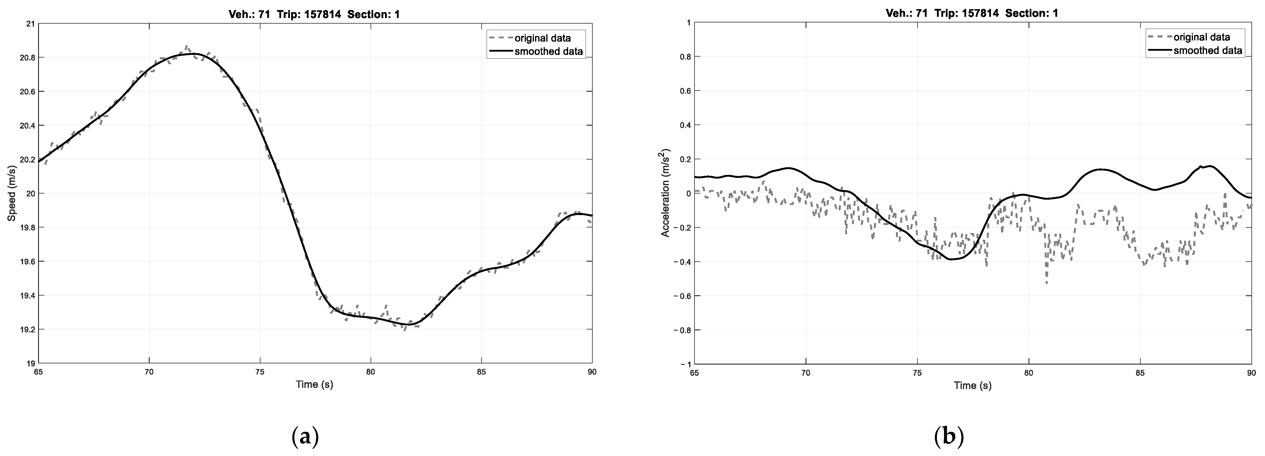
A smoothing process is performed to remove noise from the classified data. For this purpose, the locally estimated scatterplot smoothing (LOESS) algorithm, which is a widely known local regression method, is used [49]. LOESS is a regression method that constructs a quadratic polynomial using a weight function w for regression smoothing and a robust weight function G based on median values (see Equations (7)–(9)). In Equation (9), the coefficients a , b , and c of the quadratic polynomial are derived in the direction of minimizing the product of the weights and the square error of the actual data and the quadratic polynomial.
w x k = 1 x i x k d i 3 3 f o r   k = 1 , ,   n
G x k = 1 6 M I D 6 M I D < 1 0 6 M I D 1 s . t   6 M I D = y i y ^ i 6   m e d i a n   y i y ^ i
R S S x a , b , c = k w x k G x k y k a b x k c x k 2 2
Figure 3 is an example of smoothing results obtained by applying LOESS to the classified data. As shown in Figure 3, the smoothing process was carried out only to the extent that the characteristics of the data were not loose. In the case of the acceleration data, there is an offset within the data, thus there is an error even when the smoothing process is performed. For example, although the speed increases in the 65–70 s section in Figure 3a, the acceleration in the same section in Figure 3b is shown as 0, indicating that there exists an offset of the acceleration data. It is judged that this offset is caused by problems such as the measurement equipment setting and the mounting error when gathering the SPMD data set. However, in the case of the speed data, the smoothing processing showed a better result than the acceleration data. For this reason, acceleration for the data analysis is used by differentiating the smoothed speed of the data.

4.2. Analysis of Free Acceleration/Deceleration Point

Using the pre-processed data in Section 4.1, we analyzed the human drivers’ free acceleration/deceleration driving data in a situation where the vehicle in front is far away and not obstructed. Figure 4 shows the maximum acceleration/deceleration distributions of vehicles driven by human drivers derived from the randomly chosen 300 free acceleration/deceleration datasets. The speed, acceleration, and jerk data used for the analysis are presented in Figure A2. Moreover, the distributions of maximum acceleration/deceleration for each maximum section during free acceleration/deceleration are summarized in Table A1 and Table A2.
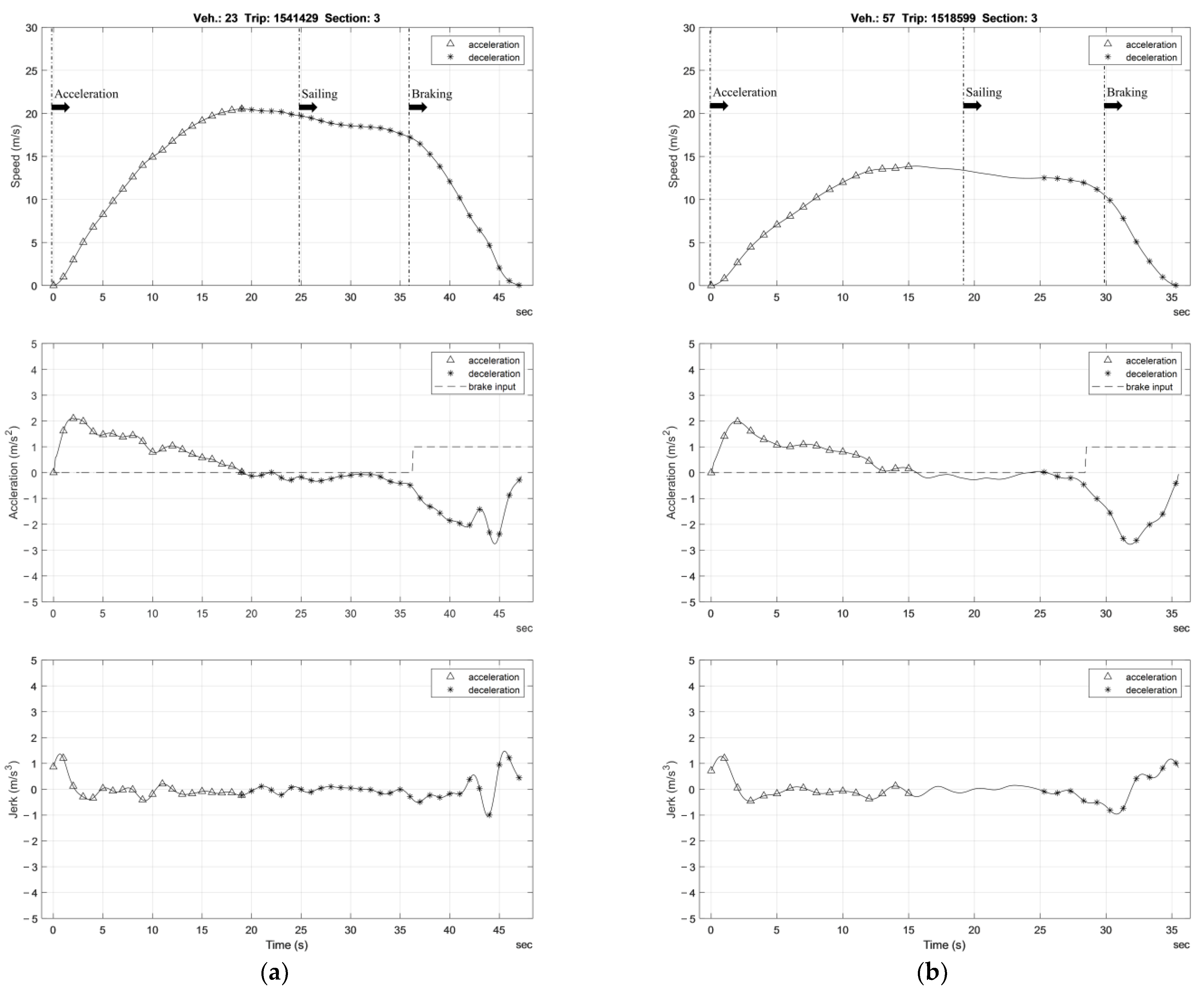
With the analysis of the free acceleration/deceleration data, human drivers generally have similar patterns during free acceleration/deceleration (see Figure A2), and the mean values of maximum acceleration/deceleration are 2.30 m/s2 and −2.16 m/s2, respectively. Longitudinal driving characteristics of human drivers can be derived mainly from the mean and median values of acceleration/deceleration, and the mean was used in this study [47,48]. Figure 5 shows the driving of different drivers arbitrarily selected to see the human drivers’ free acceleration/deceleration patterns in detail, and the maximum speed and maximum acceleration/deceleration for each driver are expressed in Table 3.
In Figure 5, the maximum acceleration/deceleration of drivers #23 and #57, which are arbitrarily chosen, demonstrate similar results to the mean values shown in Figure 4. That is, the acceleration/deceleration characteristics of typical human drivers can be defined through the criteria in Figure 4 and Table A1 and Table A2, and various acceleration/deceleration scenarios can be configured according to the analyzed distributions.

4.3. Analysis of Sailing/Braking Start Time

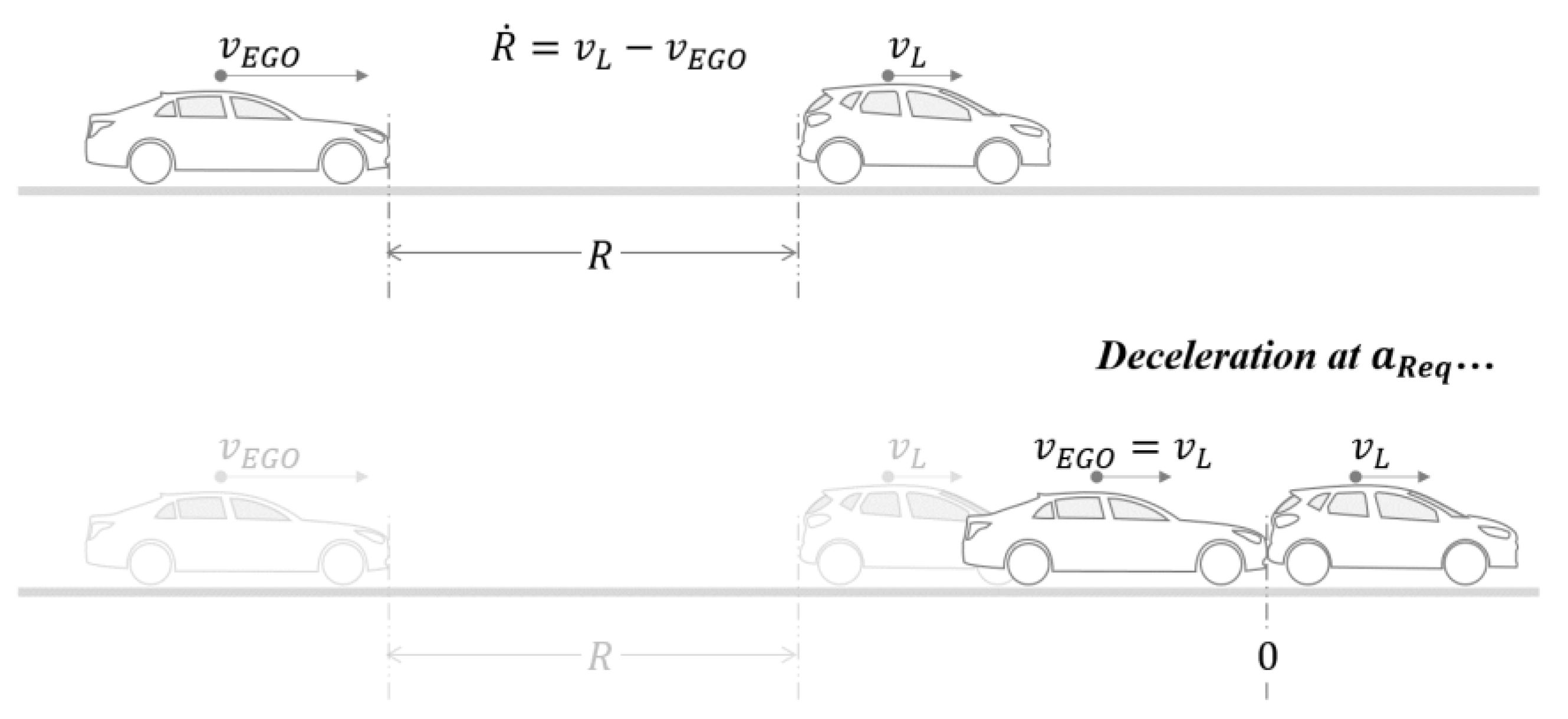
Next, we analyzed the sailing and braking start times of human drivers. In Figure 5, shown in the previous section, human drivers generally coast down before stopping, which is related to the timing of pressing the brake pedal. In other words, typical human drivers have a similar driving pattern, which sequences as acceleration, sailing, and braking. Such driving can be viewed as one of the driving characteristics derived from human drivers. To analyze the driving characteristics at the beginning of the time of braking, the required deceleration for braking is calculated and analyzed from data. The required deceleration means the deceleration required for a complete stop when the relative distance is R and the relative speed is R ˙ . Figure 6 and Equation (10) express the required deceleration calculation.
a r e q = s i g n R ˙ R ˙ 2 2 R
The beginning point of braking is defined as the point at which the first brake pedal signal occurs in the deceleration section before stopping. For the case where there is no leading vehicle, it is assumed that the virtual vehicle is stopped at the stop position of the ego vehicle. The analysis of the required deceleration calculated from the data at the beginning point of braking is specified in Figure 7a. The required deceleration at the start point of braking is −1.37 m/s2 on average with a 0.55 m/s2 standard deviation. In the same way, the required deceleration at the sailing start point before braking is analyzed. The sailing start point can be expressed as the time when the acceleration pedal is released to brake, and this can be regarded as the start point of braking. As described in Equations (2) and (3), the rolling/aerodynamic resistances affect the motion of the vehicle. Therefore, the tendency to decelerate during sailing is different depending on the size or type of the vehicle. As this study develops the longitudinal motion scenario by imitating the overall driving pattern of a human driver, the sailing behaviors of various vehicles can be expressed with the variation of the required deceleration at the sailing start point. The analysis result of the required deceleration at the start of sailing is specified in Figure 7b, and the average value is −0.89 m/s2 with a standard deviation of 0.44 m/s2. Moreover, the distributions of required deceleration at braking/sailing start point are summarized in Table A3 and Table A4.
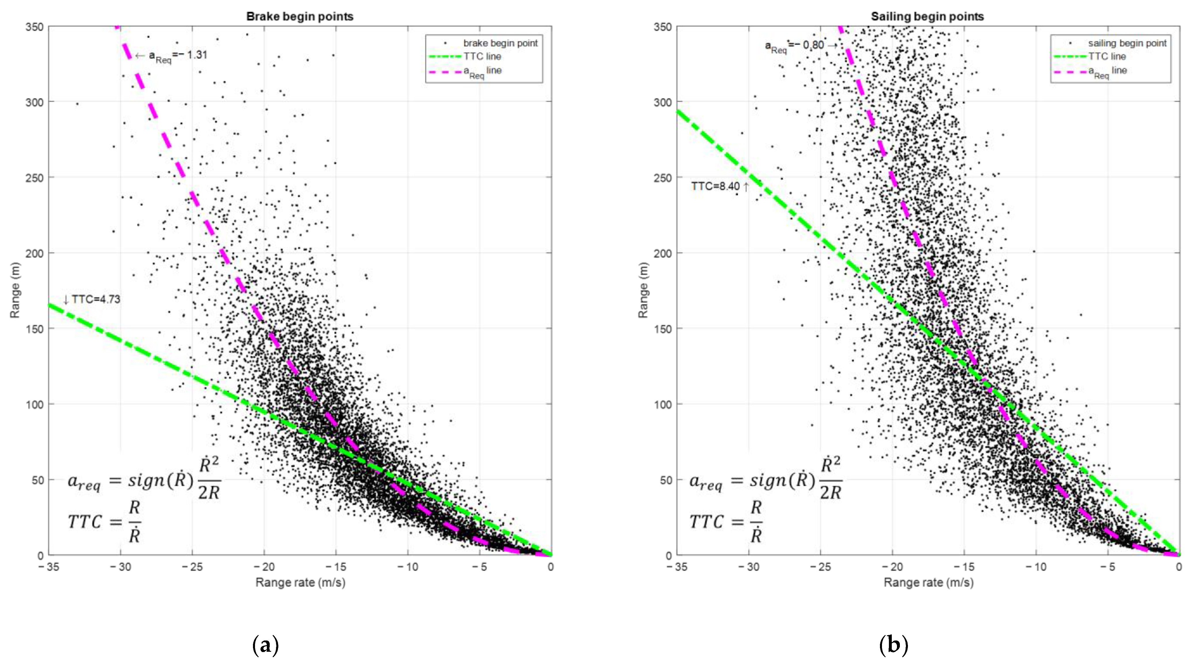
To analyze the reason why the required deceleration is necessary to imitate the driving of human drivers, the distributions of braking/sailing start points are represented with respect to relative distance/velocity (see Figure 8). Human drivers show a similar tendency to trend toward the average value of the required deceleration specified in Table A3 and Table A4. In addition, the time-to-collision (TTC), which is widely used in vehicle risk assessment standards, is approximated near the origin and compared with the specified average required deceleration. As the TTC has a linear relationship with both the relative distance and the relative speed, it cannot adequately represent the driving patterns of human drivers. In other words, to express the characteristics of the sailing and braking start points, the driver model should be an acceleration/deceleration-based model.

4.4. Driver Model Parameter Adaptation from the Analysis of Driving Data

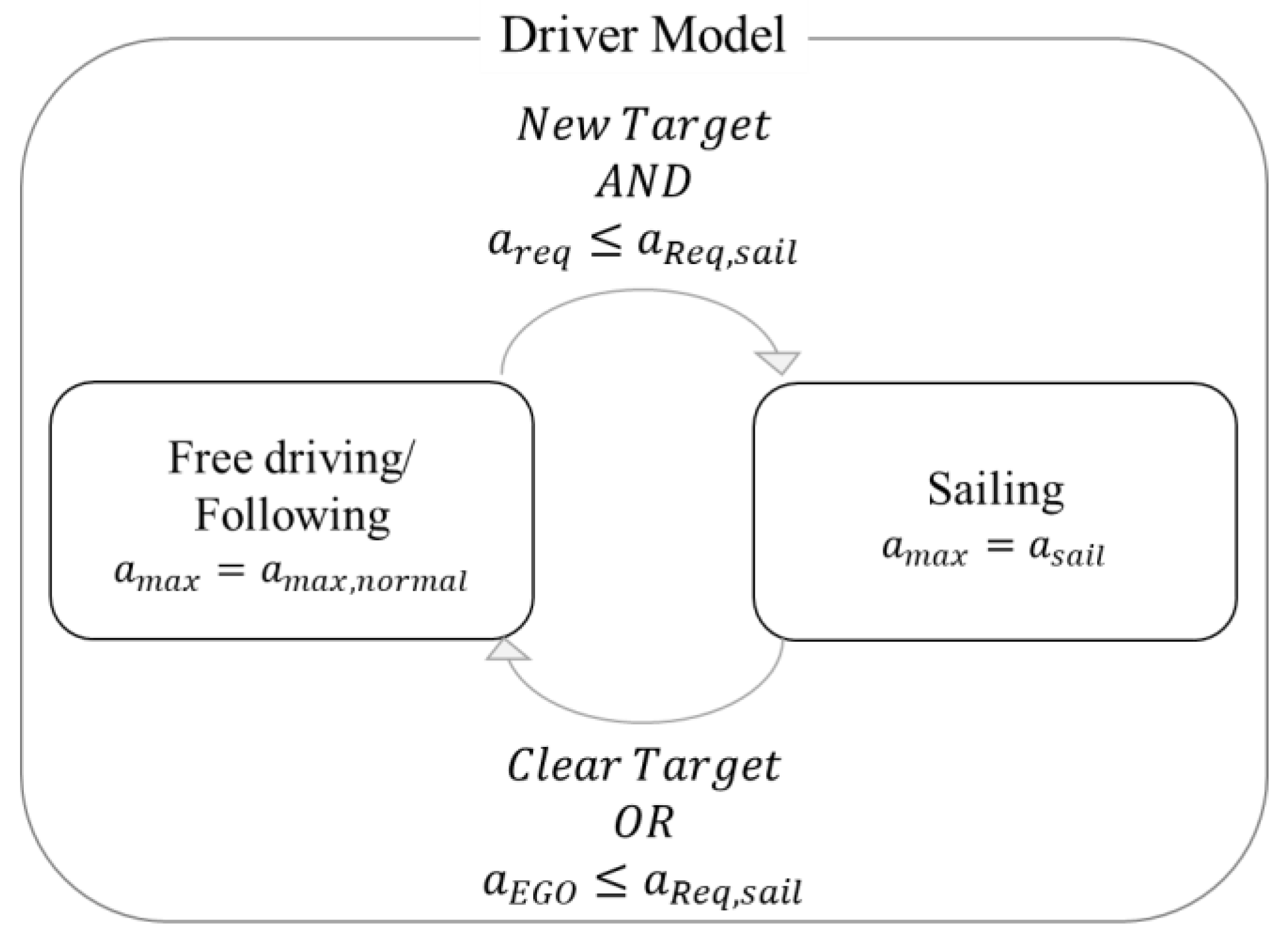
In Section 4.1, Section 4.2 and Section 4.3, parameters expressing the driving characteristics of human drivers are derived. These parameters are the maximum acceleration ( a m a x ), the maximum deceleration or minimum acceleration ( a m i n ), and the deceleration at the sailing start point ( a s a i l ). The three parameters are analyzed in terms of the mean and standard deviation in the previous sections. A typical human driver can be regarded as having the mean value of each parameter, and the more atypical the driver is, the further their behavior is from the mean. Therefore, the driving situations of various drivers can be simulated using the parameters derived from the analysis results. This means that atypical scenarios and various human driving patterns can be expressed according to changing parameters, such as the constraint for acceleration/deceleration and the weights of the driver model in the proposed longitudinal motion scenario design method. In other words, it is possible to create various longitudinal scenarios by defining the mode transition conditions of the driver model, as shown in Figure 9, and changing the constraint settings presented in Equation (6) for the required acceleration/deceleration corresponding to each mode.
There is a limit to expressing the driving patterns of various drivers only by setting the constraints. Thus, as shown in Equation (11), they can be expressed by changing the weights of the MPC used in the driver model design.
Q = q 1 0 0 q 2 ,     R = r 1
q 1 and q 2 are weights for the distance error and velocity error, respectively, and r 1 is a weight for acceleration, which is a control input. In linear quadratic-based optimal control, suitable control performance is derived with the ratio of each weight. Therefore, in this study, the driving pattern is simulated by changing only q 1 and r 1 , while fixing the weight of the velocity error q 2 as 1 [46]. When the driver’s velocity to be imitated in the simulation is v v e l o , d a t a , the weights q 1 and r 1 of the driver model can be derived using the following equation. Here, T is the length of the time interval to be imitated, and v m o d e l is the speed of the driver model.
q 1 * ,   r 1 * = arg min q 1 ,   r 1 1 T k = 1 T v v e l o , d a t a k v m o d e l k 2

5. Computer Simulation Results

To verify the proposed longitudinal motion scenario design method, we set appropriate parameters in the driver model to check whether the driving is like that of a human driver. The Gipps model introduced in Table 1 is used for comparison, and the parameters common to both the Gipps model and the MPC-based driver model are set to the same values [28]. The computer simulation was conducted assuming the driving situation on a dry, asphalt, straight road.
The simulations are carried out with Intel® CoreTM [email protected] GHz, 32 GB RAM. The execution time was derived with 22 ms as the maximum, 0.64 ms as the minimum, and 0.92 ms as the mean per step, which is less than the step time specified as 200 ms (0.2 s) for the overall simulation results. For this reason, real-time performance can be guaranteed during simulation. If the execution is performed with explicit MPC, it is expected to derive less than the preciously derived execution time. Generally, the driving tendency of human drivers can vary depending on the driving situation [47,48]. For this reason, the simulation results were expressed as fixed parameters and constraints for the randomly selected acceleration/deceleration section of the human driving data.
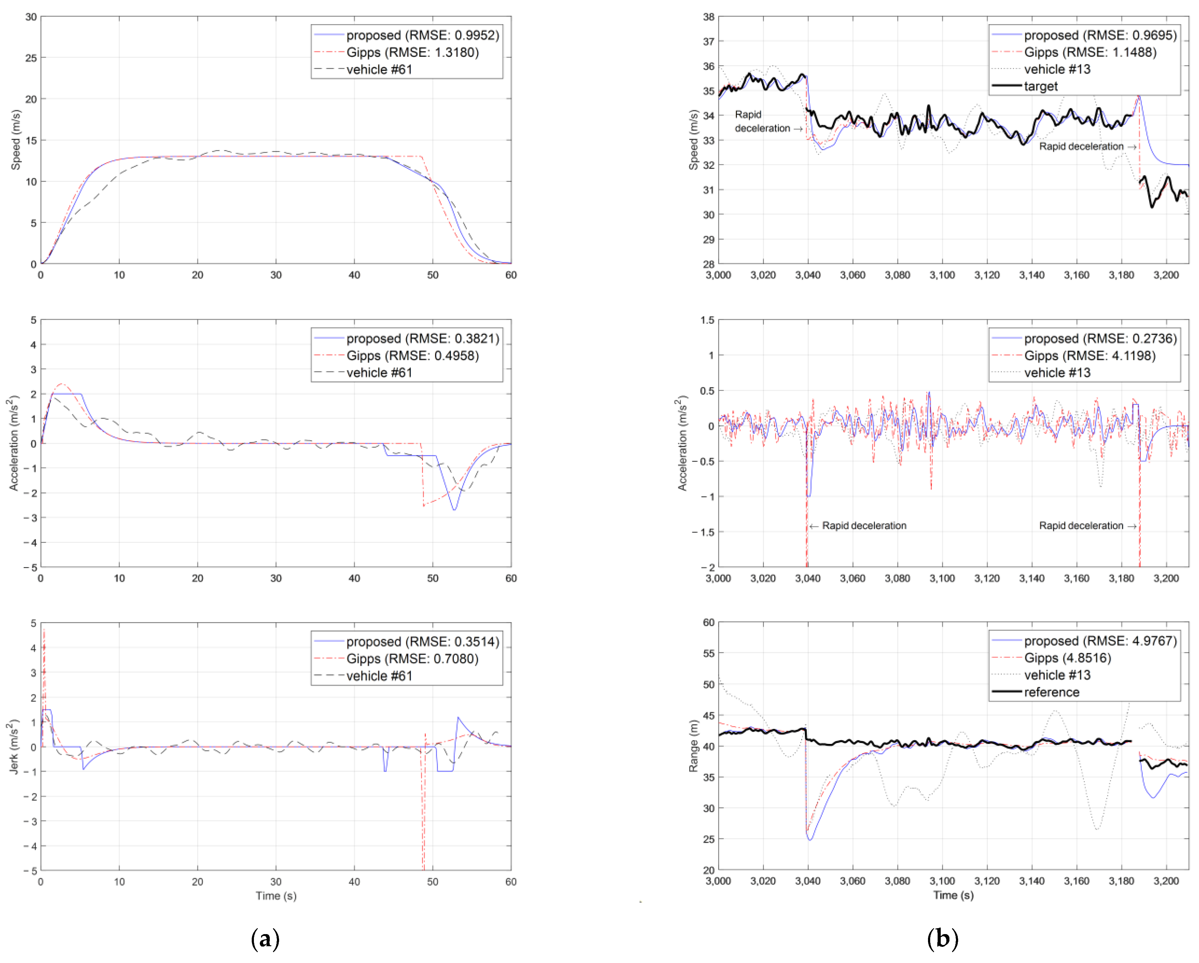
The simulation results are compared with the results imitating the driving data of drivers #23, #57, #61, and #13 of SPMD, and are presented in Figure 10 and Figure 11. The weights of the proposed MPC-based driver model were derived using Equation (12) to show the longitudinal driving pattern most similar to the actual driver’s speed profile. The parameters set in the MPC-based driver model are specified in Table 4. It can be confirmed that the accelerations shown in Table 4 are included in the acceleration range of human drivers derived from Section 4. In these results, the proposed model has mostly lower RMSE than the Gipps model’s, which means that the proposed model shows a more similar driving pattern than the Gipps model. With the simulation results from Figure 10 and Figure 11a, it is shown that the proposed model can simulate both the acceleration and the deceleration of the target driver, as well as the timing and deceleration of the driving speed. However, the Gipps model shows a sudden acceleration/deceleration change that is physically impossible due to the absence of constraints. In other words, the Gipps model shows a large value of jerks when the vehicle starts acceleration and braking. Moreover, the sailing shown by the human driver is not considered in the Gipps model, resulting in differences between the Gipps model predictions and the actual human driver behavior. If the Gipps model is used in the verification of ADAS and ADS, the ADAS and ADS can act abnormally because the Gipps model acts in a manner that is physically impossible in the real world. For this reason, the proposed method can be reasonable in the verification of ADAS and ADS.
The proposed driver model is verified with the presence of multiple lane changes in the SPMD data, which is driver #13’s driving, to confirm the driving reliability in the traffic environment (see Figure 11b). The leading vehicle with a relatively low speed changes into a lane ahead of the ego vehicle at 3040 s and 3190 s. In the case of the proposed model, the change in acceleration is similar to that of driver #13’s driving, and stable driving is achieved for the leading vehicle. However, the Gipps model shows rapid acceleration changes due to the mode transition when a lane change occurs. This shows the same result as the problem shown in Figure 10 and Figure 11a. The RMSE of the proposed method is similar to the Gipps’. This is because the proposed method is assumed with the constant velocity motion of the leading vehicle ( v L ,   a L 0 ) for simplification. Moreover, driver #13’s driving is not shown to have the CTG policy to the leading vehicle as the proposed model. However, the proposed model has a similar acceleration tendency as the human driver, despite the presence of the velocity/acceleration of the leading vehicle. If the leading vehicle has a sudden velocity change, the acceleration of the leading vehicle should be considered in the driver model, as mentioned in Section 3.1, for more realistic driving motion.
With the computer simulation results, the proposed longitudinal motion scenario design method not only simulates sailing and the longitudinal driving characteristics of human drivers, but it also satisfies the constraints. In addition, with variations of the constraints and weights of the driver model, it is confirmed that various human drivers can be imitated. Moreover, the proposed model can induce an atypical scenario if the constraints and weights are suitably chosen. For these reasons, this method can simulate the longitudinal movement of surrounding vehicles of the ego vehicle more diversely and realistically in a simulation environment. With these results, we confirmed that the possibility of designing various longitudinal scenarios with human driving characteristics. This method is focused on typical longitudinal driving situations. However, it is judged that malicious driving situations or edge cases can be dealt with if the constraint is set to approximate the vehicle’s limit situation or collision risk situation, or if the target acceleration/deceleration is approximated to the limit situation, by diversifying the weights of the driver model. Therefore, the proposed method can provide more realistic scenarios by overcoming the shortcomings in the existing scenario design methods. However, as these results were compared with the randomly selected drivers in the limited driving section, additional verification is required for the robustness of the proposed method. Due to this, further improvement and verification will be conducted in future work.

6. Conclusions

In this paper, a longitudinal motion scenario design method was proposed to overcome the shortcomings of the existing scenarios for ADAS and ADS verification. A simplified vehicle model was designed, including the dynamic characteristics of the vehicle that provide physical constraints, and the longitudinal driver model to control it was designed based on the MPC. The longitudinal driver model parameters were derived from a large-scale driving database to overcome the limitations of the conventional traffic models. To obtain reliable model parameters, the human drivers’ acceleration/deceleration tendency and constraints were derived through the analysis of pre-processed data. The proposed longitudinal motion scenario design method showed an organic relationship with the test vehicle and other vehicles in the scenario, and at the same time can define atypical conditions more clearly and intuitively, which is meaningful in conducting more free and realistic tests. In addition, the proposed method can simulate various driving situations by simply changing parameters, without having to configure a complex vehicle dynamics model or driver model.
The proposed method was validated in the computer simulation environment. The MPC, which is used in the driver model design, may have difficulty satisfying real-time performance due to the high amount of computation if the driving situation is more complex. For this reason, it can be supplemented by using explicit MPC or other constraint control methods, such as the control barrier function method [46]. Moreover, in this study, only the longitudinal aspect of the vehicle was considered to derive the driving characteristics of human drivers. However, human drivers also have lateral characteristics in the real world, such as two-dimensional trajectories in a lane change situation. Therefore, future work should develop an adaptive scenario design method to consider both longitudinal and lateral driving scenarios.

Author Contributions

Formal analysis, K.C. and C.P.; project administration, K.C., C.P. and H.L.; software, K.C. and C.P.; validation, K.C. and C.P.; writing—original draft preparation, K.C. and C.P.; writing—review and editing, K.C. and H.L.; supervision, H.L. All authors have read and agreed to the published version of the manuscript.

Funding

This research received no external funding.

Institutional Review Board Statement

Not applicable.

Informed Consent Statement

Not applicable.

Data Availability Statement

Not applicable.

Acknowledgments

This work was supported by the Autonomous Driving Development Innovation Program (20014476, Development of Mixed Reality-based Autonomous Driving Parts and System Evaluation Technology) funded by the Ministry of Trade, Industry & Energy (MOTIE, Korea).

Conflicts of Interest

The authors declare no conflict of interest.

Appendix A

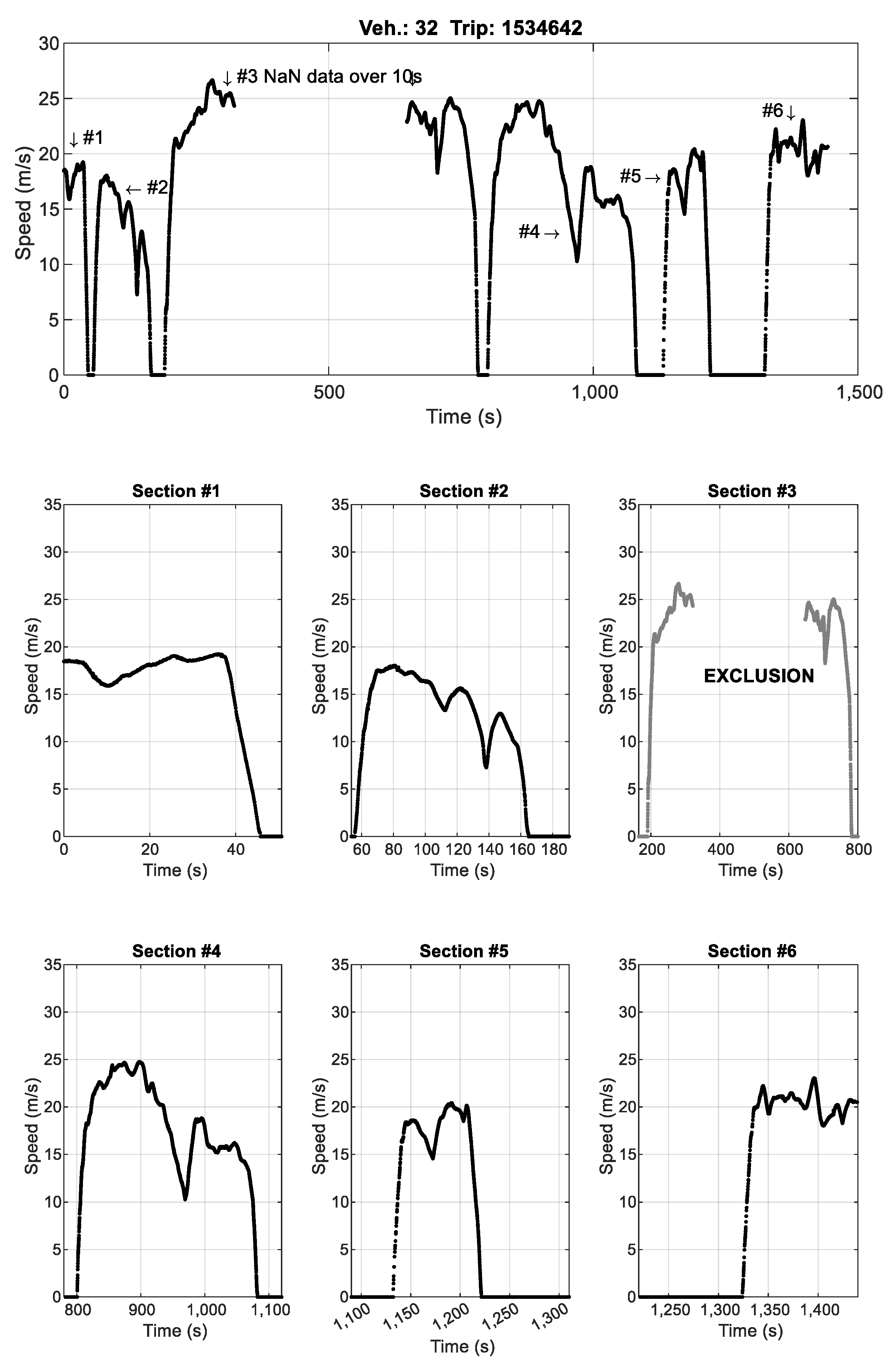
This is a description of the data classification process of SPMD for human driver driving characteristic analysis. For data classification, it is based on speed and radar data. First, as the driving characteristics of human drivers are not well expressed when the length of the data is short, data of less than 300 s were excluded. Moreover, due to the problem of the dataset itself, the case where there was no radar data measuring surrounding vehicles was excluded. Next, the data was classified by excluding the situation where the speed, which is judged as stop, was 0 and the data did not continue for more than 10 s. For example, section #3 of Figure A1 is excluded from the data for driving characteristics analysis because the data does not continue for more than 10 s.
Figure A1. Example of the data exclusion process for the case of SPME driver #32.
Applsci 13 00716 g0a1
Figure A2. 300 randomly sampled data of free acceleration/deceleration situation from SPMD: (a) case of free acceleration; (b) case of free deceleration.
Applsci 13 00716 g0a2
Figure A2 shows 300 randomly sampled datasets from SPMD for the free acceleration/deceleration characteristics of human drivers in Section 4.2. Table A1, Table A2, Table A3 and Table A4 are the distributions of maximum acceleration, deceleration, required deceleration at the braking start point, and required deceleration at the sailing start point, respectively.
Table A1. Distribution of maximum acceleration (300 random vehicles, free acceleration).
Range
(m/s)
Bottom75%Med.25%Top
100.131.111.572.063.47
10–201.032.042.382.763.83
20–301.232.322.673.094.24
30–401.632.392.733.184.076
ALL0.5671.862.302.734.02
Table A2. Distribution of maximum deceleration (300 random vehicles, free deceleration).
Range
(m/s)
Bottom75%Med.25%Top
10−4.85−1.90−1.49−1.08−0.15
10–20−3.73−2.57−2.16−1.80−0.95
20–30−4.36−3.03−2.52−2.13−0.98
30–40−3.99−3.08−2.62−2.21−1.38
ALL−3.85−2.56−2.10−1.68−0.36
Table A3. The distribution of the required acceleration at the braking start point.
Range
(m/s)
Bottom75%Med.25%Top
10−2.16−1.27−0.98−0.67−0.03
10–20−2.56−1.67−1.36−1.11−0.33
20–30−2.80−1.88−1.54−1.27−0.38
30–40−2.47−1.69−1.20−0.86−0.46
ALL−2.57−1.65−1.31−1.04−0.12
Table A4. The distribution of the required acceleration at the sailing start point.
Range
(m/s)
Bottom75%Med.25%Top
10−1.67−0.96−0.70−0.47−0.03
10–20−1.88−1.13−0.84−0.63−0.21
20–30−0.83−1.12−0.84−0.65−0.20
30–40−1.24−0.82−0.64−0.50−0.17
ALL−1.81−1.08−0.80−0.60−0.03

References

  1. Pendleton, S.D.; Andersen, H.; Du, X.; Shen, X.; Meghjani, M.; Eng, Y.H.; Rus, D.; Ang, M.H. Perception, Planning, Control, and Coordination for Autonomous Vehicles. Machines 2017, 5, 6. [Google Scholar] [CrossRef]
  2. Fényes, D.; Németh, B.; Gáspár, P. A Novel Data-Driven Modeling and Control Design Method for Autonomous Vehicles. Energies 2021, 14, 517. [Google Scholar] [CrossRef]
  3. Nie, Z.; Farzaneh, H. Adaptive Cruise Control for Eco-Driving Based on Model Predictive Control Algorithm. Appl. Sci. 2020, 10, 5271. [Google Scholar] [CrossRef]
  4. Wang, P.; Gao, S.; Li, L.; Sun, B.; Cheng, S. Obstacle Avoidance Path Planning Design for Autonomous Driving Vehicles Based on an Improved Artificial Potential Field Algorithm. Energies 2019, 12, 2342. [Google Scholar] [CrossRef] [Green Version]
  5. Kuutti, S.; Bowden, R.; Jin, Y.; Barber, P.; Fallah, S. A Survey of Deep Learning Applications to Autonomous Vehicle Control. IEEE Trans. Intell. Transp. Syst. 2021, 22, 712–733. [Google Scholar] [CrossRef]
  6. Dosovitskiy, A.; Ros, G.; Codevilla, F.; Lopez, A.; Koltun, V. CARLA: An Open Urban Driving Simulator. In Proceedings of the 1st Annual Conference on Robot Learning; PMLR, Mountain View, CA, USA, 13–15 November 2017; pp. 1–16. [Google Scholar]
  7. Zapridou, E.; Bartocci, E.; Katsaros, P. Runtime Verification of Autonomous Driving Systems in CARLA. In Proceedings of the Runtime Verification, Los Angeles, CA, USA, 6–9 October 2020; Deshmukh, J., Ničković, D., Eds.; Springer International Publishing: Cham, Switzerland, 2020; pp. 172–183. [Google Scholar]
  8. Arcidiacono, A. ADAS Virtual Validation: ACC and AEB Case Study with IPG CarMaker. Master’s Thesis, Politecnico di Torino, Turin, Italy, 2018. [Google Scholar]
  9. Zhou, J.; Schmied, R.; Sandalek, A.; Kokal, H.; del Re, L. A Framework for Virtual Testing of ADAS. SAE Int. J. Passeng. Cars Electron. Electr. Syst. 2016, 9, 66–74. [Google Scholar] [CrossRef]
  10. Park, C.; Chung, S.; Lee, H. Vehicle-in-the-Loop in Global Coordinates for Advanced Driver Assistance System. Appl. Sci. 2020, 10, 2645. [Google Scholar] [CrossRef] [Green Version]
  11. Siegl, S.; Ratz, S.; Düser, T.; Hettel, R. Vehicle-in-the-Loop at Testbeds for ADAS/AD Validation. ATZ Electron. Worldw 2021, 16, 62–67. [Google Scholar] [CrossRef]
  12. Tettamanti, T.; Szalai, M.; Vass, S.; Tihanyi, V. Vehicle-in-the-Loop Test Environment for Autonomous Driving with Microscopic Traffic Simulation. In Proceedings of the 2018 IEEE International Conference on Vehicular Electronics and Safety (ICVES), Madrid, Spain, 12–14 September 2018; pp. 1–6. [Google Scholar]
  13. Van Ratingen, M.R. The Euro Ncap Safety Rating. In Karosseriebautage Hamburg 2017; Springer: Berlin, Germany, 2017; pp. 11–20. [Google Scholar]
  14. ISO. Intelligent Transport Systems–Adaptive Cruise Control Systems–Performance Requirements and Test Procedures; ISO: Geneva, Switzerland, 2018. [Google Scholar]
  15. Hulshof, W.; Knight, I.; Edwards, A.; Avery, M.; Grover, C. Autonomous Emergency Braking Test Results. In Proceedings of the 23rd International Technical Conference on the Enhanced Safety of Vehicles (ESV), Seoul, Republic of Korea, 27–30 May 2013; National Highway Traffic Safety Administration: Washington, DC, USA, 2013; pp. 1–13. [Google Scholar]
  16. Zhao, D. Accelerated Evaluation of Automated Vehicles. Ph.D. Thesis, University of Michigan, Ann Arbor, MI, USA, 2016. [Google Scholar]
  17. Peng, H.; Leblanc, D. Evaluation of the Performance and Safety of Automated Vehicles. White Paper on NSF Transportation CPS Work. 2012. Available online: https://cps-vo.org/sites/default/files/webform/Evaluation_of_the_Performance_and_Safety_of_Automated_Vehicles_0.pdf (accessed on 16 December 2022).
  18. Lee, K. Longitudinal Driver Model and Collision Warning and Avoidance Algorithms Based on Human Driving Databases; University of Michigan: Ann Arbor, MI, USA, 2004. [Google Scholar]
  19. Klischat, M.; Althoff, M. Generating Critical Test Scenarios for Automated Vehicles with Evolutionary Algorithms. In Proceedings of the 2019 IEEE Intelligent Vehicles Symposium (IV), Paris, France, 9–12 June 2019; pp. 2352–2358. [Google Scholar]
  20. Koopman, P.; Wagner, M. Challenges in Autonomous Vehicle Testing and Validation. SAE Int. J. Transp. Safety 2016, 4, 15–24. [Google Scholar] [CrossRef] [Green Version]
  21. Riedmaier, S.; Ponn, T.; Ludwig, D.; Schick, B.; Diermeyer, F. Survey on Scenario-Based Safety Assessment of Automated Vehicles. IEEE Access 2020, 8, 87456–87477. [Google Scholar] [CrossRef]
  22. Fellendorf, M.; Vortisch, P. Microscopic Traffic Flow Simulator VISSIM. In Fundamentals of Traffic Simulation; Springer: Berlin, Germany, 2010; pp. 63–93. [Google Scholar]
  23. Kaths, J.; Krause, S. Integrated Simulation of Microscopic Traffic Flow and Vehicle Dynamics. In Proceedings of the IPG Apply & Innovate 2016, Karlsruhe, Germany, 20–21 September 2016. [Google Scholar]
  24. Pipes, L.A. An Operational Analysis of Traffic Dynamics. J. Appl. Phys. 1953, 24, 274–281. [Google Scholar] [CrossRef]
  25. Gazis, D.C.; Herman, R.; Rothery, R.W. Nonlinear Follow-the-Leader Models of Traffic Flow. Oper. Res. 1961, 9, 545–567. [Google Scholar] [CrossRef]
  26. Newell, G.F. Nonlinear Effects in the Dynamics of Car Following. Oper. Res. 1961, 9, 209–229. [Google Scholar] [CrossRef]
  27. Tyler, J. The Characteristics of Model-Following Systems as Synthesized by Optimal Control. IEEE Trans. Autom. Control. 1964, 9, 485–498. [Google Scholar] [CrossRef]
  28. Gipps, P.G. A Behavioural Car-Following Model for Computer Simulation. Transp. Res. Part B Methodol. 1981, 15, 105–111. [Google Scholar] [CrossRef]
  29. Ahmed, H.U.; Huang, Y.; Lu, P. A Review of Car-Following Models and Modeling Tools for Human and Autonomous-Ready Driving Behaviors in Micro-Simulation. Smart Cities 2021, 4, 314–335. [Google Scholar] [CrossRef]
  30. Dingus, T.A.; Klauer, S.G.; Neale, V.L.; Vicki, L.; Petersen, A.; Lee, S.E.; Sudweeks, J.; Perez, M.A.; Hankey, J.; Ramsey, D.; et al. The 100-Car Naturalistic Driving Study, Phase II Results of the 100-Car Field Experiment; National Highway Traffic Safety Administration: Washington, DC, USA, 2006.
  31. Ervin, R.; Sayer, J.; LeBlanc, D.; Bogard, S.; Mefford, M.; Hagan, M.; Bareket, Z.; Winkler, C. Automotive Collision Avoidance System Field Operational Test Report: Methodology and Results; Transportation Research Board: Washington, DC, USA, 2005. [Google Scholar]
  32. LeBlanc, D.J. Road Departure Crash Warning System Field Operational Test: Methodology and Results. Volume 1: Technical Report; Transportation Research Institute, University of Michigan: Ann Arbor, MI, USA, 2006. [Google Scholar]
  33. Victor, T.; Bärgman, J.; Hjälmdahl, M.; Kircher, K.; Svanberg, E.; Hurtig, S.; Gellerman, H.; Moeschlin, F. Sweden-Michigan Naturalistic Field Operational Test (Semifot) Phase 1: Final Report; Chalmers: Goteborg, Sweden, 2010. [Google Scholar]
  34. Sayer, J.; LeBlanc, D.; Bogard, S.; Funkhouser, D.; Bao, S.; Buonarosa, M.L.; Blankespoor, A. Integrated Vehicle-Based Safety Systems Field Operational Test: Final Program Report; Transportation Research Institute, University of Michigan: Ann Arbor, MI, USA, 2011. [Google Scholar]
  35. Bezzina, D.; Sayer, J. Safety Pilot Model Deployment: Test Conductor Team Report. Report No. DOT HS 2014, 812, 18. [Google Scholar]
  36. Traffic Analysis Tools: Next Generation Simulation-FHWA Operations. Available online: https://ops.fhwa.dot.gov/trafficanalysistools/ngsim.htm (accessed on 20 October 2022).
  37. Open Dataset. Available online: https://waymo.com/open/ (accessed on 20 October 2022).
  38. Krajewski, R.; Bock, J.; Kloeker, L.; Eckstein, L. The HighD Dataset: A Drone Dataset of Naturalistic Vehicle Trajectories on German Highways for Validation of Highly Automated Driving Systems. In Proceedings of the 2018 21st International Conference on Intelligent Transportation Systems (ITSC), Maui, HI, USA, 4–7 November 2018; pp. 2118–2125. [Google Scholar]
  39. Bifulco, G.N.; Simonelli, F.; Di Pace, R. Experiments toward an Human-like Adaptive Cruise Control. In Proceedings of the 2008 IEEE Intelligent Vehicles Symposium, Eindhoven, The Netherlands, 4–6 June 2008; pp. 919–924. [Google Scholar]
  40. Zheng, J.; Suzuki, K.; Fujita, M. Car-Following Behavior with Instantaneous Driver–Vehicle Reaction Delay: A Neural-Network-Based Methodology. Transp. Res. Part C Emerg. Technol. 2013, 36, 339–351. [Google Scholar] [CrossRef]
  41. He, Z.; Zheng, L.; Guan, W. A Simple Nonparametric Car-Following Model Driven by Field Data. Transp. Res. Part B Methodol. 2015, 80, 185–201. [Google Scholar] [CrossRef]
  42. Przybyla, J.; Taylor, J.; Jupe, J.; Zhou, X. Estimating Risk Effects of Driving Distraction: A Dynamic Errorable Car-Following Model. Transp. Res. Part C Emerg. Technol. 2015, 50, 117–129. [Google Scholar] [CrossRef]
  43. Rajamani, R. Vehicle Dynamics and Control; Mechanical Engineering Series; Springer: Boston, MA, USA, 2012; ISBN 978-1-4614-1432-2. [Google Scholar]
  44. Kiencke, U.; Nielsen, L. Automotive Control Systems: For Engine, Driveline, and Vehicle; IOP Publishing Ltd.: Bristol, UK, 2000. [Google Scholar]
  45. Yi, K.; Song, B. Automated Driving Vehicles. In Vehicle Dynamics: Fundamentals and Ultimate Trends; Lenzo, B., Ed.; CISM International Centre for Mechanical Sciences; Springer International Publishing: Cham, Switzerland, 2022; pp. 289–387. ISBN 978-3-030-75884-4. [Google Scholar]
  46. Borrelli, F.; Bemporad, A.; Morari, M. Predictive Control for Linear and Hybrid Systems; Cambridge University Press: Cambridge, UK, 2017. [Google Scholar]
  47. Bosetti, P.; Da Lio, M.; Saroldi, A. On the Human Control of Vehicles: An Experimental Study of Acceleration. Eur. Transp. Res. Rev. 2014, 6, 157–170. [Google Scholar] [CrossRef]
  48. Xia, L.; Li, P.; Su, Z.; Chen, T.; Deng, Z.; Sun, D. Longitudinal Driving Behavior before, during, and after a Left-Turn Movement at Signalized Intersections: A Naturalistic Driving Study in China. Sustainability 2022, 14, 11630. [Google Scholar] [CrossRef]
  49. Loader, C. Local Regression and Likelihood; Springer Science & Business Media: Berlin, Germany, 2006. [Google Scholar]
Figure 1. Constraints of longitudinal force and acceleration: (a) the constraint of longitudinal force varies with the transmission gear ratio; (b) the simplified acceleration constraint for the vehicle model.
Applsci 13 00716 g001
Figure 2. The scheme of error dynamics for the car-following model.
Applsci 13 00716 g002
Figure 3. Example of pre-processed driving data: (a) speed; (b) acceleration.
Applsci 13 00716 g003
Figure 4. Distribution of maximum acceleration/deceleration (300 random vehicles): (a) case of free acceleration; (b) case of free deceleration.
Applsci 13 00716 g004
Figure 5. Examples of free acceleration/deceleration driving cases: (a) case of SPMD driver #23; (b) case of SPMD driver #57.
Applsci 13 00716 g005
Figure 6. Scheme of required deceleration.
Applsci 13 00716 g006
Figure 7. Distribution of required deceleration (300 random vehicles): (a) case of braking start point; (b) case of sailing start point.
Applsci 13 00716 g007
Figure 8. Distributions of braking/sailing start point w.r.t. relative distance/velocity: (a) the case of the braking start point; (b) the case of the sailing start point.
Applsci 13 00716 g008
Figure 9. Scheme of the driver model for the proposed longitudinal motion scenario design.
Applsci 13 00716 g009
Figure 10. Computer simulation results to compare the Gipps model (compared) and the proposed driver model (proposed): (a) the case of SPMD driver #23; (b) the case of SPMD driver #57.
Applsci 13 00716 g010
Figure 11. Computer simulation results to compare the Gipps model (compared) and the proposed driver model (proposed): (a) the case of SPMD driver #61; (b) the case of SPMD driver #13 (cut-in/out situation).
Applsci 13 00716 g011
Table 1. Deterministic classical car-following models.
Researcher
(Year)
Model
Pipe [24]
(1953)
a F t + τ = C R ˙ t
Gazis [25]
(1961)
a F t + τ = C R ˙ t v F t m R t l
Newell [26]
(1961)
v F t + τ = V d · 1 exp C · R t R m i n V d
Tyler [27]
(1964)
a F t + τ = C V · R ˙ t + C S · R t C t · v F t
Gipps [28]
(1981)
v F t + τ = min v F t + 2.5 · A · τ · 1 v F t v d · 0.025 + v F t V d B · τ + B 2 · τ 2 B · 2 · R t R m i n v F t · τ v L t 2 B ^
Table 2. Data classification process to ensure reliability.
StepExclusion ConditionsRemain Time (s)
(1) Original-8,338,419.4
(2) Trip timeTrip data less than 300 s7,589,392.0
(3) RadarRadar data nonexistence7,523,291.5
(4) 0 to 0Zero speed nonexistence7,277,452.8
(5) DataContinuous data nonexistence over 10 s6,884,491.7
Table 3. Summary of two drivers’ trips.
Trip Time
(s)
Max. Speed
(m/s)
Max. Acceleration
(m/s2)
Max. Deceleration
(m/s2)
Driver #2347.220.52.10−2.75
Driver #5735.513.91.98−1.92
Table 4. Driver model parameters for simulation.
a m a x ( m / s 2 ) a m i n ( m / s 2 ) a r e q ,   s a i l ( m / s 2 ) a s a i l ( m / s 2 ) q 1 ( - ) r 1 ( - )
Driver #232−2.1−0.5−0.4345
Driver #572−2.5−0.5−0.1545
Driver #612−2.7−0.8−0.5240
Driver #132−1−0.5−0.1540
Disclaimer/Publisher’s Note: The statements, opinions and data contained in all publications are solely those of the individual author(s) and contributor(s) and not of MDPI and/or the editor(s). MDPI and/or the editor(s) disclaim responsibility for any injury to people or property resulting from any ideas, methods, instructions or products referred to in the content.