Full-Field Mode Shape Identification Based on Subpixel Edge Detection and Tracking

Abstract

Most research on computer vision (CV)-based vibration measurement is limited to the determination of discrete or coarse mode shapes of the structure. The continuous edge of the structure in images has rich optical features, and thus, by identifying and tracking the movement of the structure’s edge, it is possible to determine high-resolution full-field mode shapes of the structure without a preset target. The present study proposes a CV-based method of full-field mode shape identification using the subpixel edge detection and tracking techniques. Firstly, the Canny operator is applied on each frame of the structure vibration video to extract the pixel-level edges, and the improved Zernike orthogonal moment (ZOM) subpixel edge detection technique is adopted to relocate the precise structure edges. Then, all the detected edge points are tracked to obtain the full-field dense displacement time history that is subsequently used to determine the structure frequencies and compute full-field mode shapes by combining the covariance driven stochastic subspace identification (SSI-COV) with the hierarchical cluster analysis. Finally, the proposed method is verified on the aluminum cantilever beam in the laboratory and the Humen Bridge in the field. The results show that the proposed method is able to detect more precise structure edges and identify the full-field displacement and mode shapes of structures without the need for installing artificial targets on the structure in advance, which provides valuable information for the structural condition assessment, especially for structures with small-amplitude vibrations.

1. Introduction

Large-scale (long-span or high-rise) engineering structures are prone to vibrate under external loadings such as wind, earthquake, traffic, etc. These vibrations can cause damage (e.g., fatigue and cracking) to the structural components, which can lead to the destruction of the structure, resulting in huge economic losses [1,2]. The monitoring of structural vibration and modal properties can provide crucial information both for the evaluation of structural safety and for maintenance purposes in civil engineering [3,4]. Therefore, the accurate determination of vibration displacements and modal parameters is of great importance to the structural condition assessment during its service life.

Traditionally, the vibration response of structures has mainly been measured through contact sensors (e.g., accelerometers or linear variable differential transducer (LVDT) [5]. However, these contact-type sensors need to be installed at specific locations on structures, which is often difficult or even impossible in some cases. Recently, the non-contact sensing system based on computer vision (CV) has been developed and applied to vibration measurement [6,7,8]. The CV-based photogrammetry techniques for structural vibration measurement mainly include the template-matching method [9], digital image correlation (DIC) [10], and the optical flow method [11]. Feng et al. [12] adopted the template-matching algorithm with upsampled cross-correlation to determine the structural displacement by tracking the artificial target on the structure and verified its feasibility on a steel frame in the laboratory [13]. The DIC method uses dense speckle patterns as artificial targets on the structure surface and calculates the grayscale variations to acquire the vibration response [14]. The above methods require manually adding high-contrast patterns on the test object as optical targets for CV processing. To address this limitation, many researchers utilize the internal features of the test object to perform the optical measurement. The optical flow method is one such method that works by calculating the brightness variation of pixels in image sequences [15]. Caetano et al. [16] used this method [17] to measure the displacement of the region of interest (ROI) on cables without the set of any targets, and the reverse synthesis algorithm was used to further reduce the computation time [18]. Although the full-field optical flow method stated above can compute the Eulerian velocity field of the whole image, the computational time is too long for online monitoring. Hence, Cha et al. [19] adopted the phase-based optical flow algorithm to measure the displacement of a few specific pixels in the image. Guo et al. [20] employed deep learning to automatically select pixels for target tracking to obtain the vibration displacement time history of the structure, which was verified in laboratory experiments.

Most research on CV-based vibration measurement is limited to the determination of the displacement or frequencies of vibrating structures. The mode shapes of structures are also critical indicators for structural health monitoring and damage detection. Recently, a few researchers have developed CV-based methods for the identification of structural mode shapes. Dong et al. [21] used the template-matching method to synchronously measure the dynamic displacements of the structure at various locations to identify mode shapes of a simply supported rectangular steel girder. Yoon et al. [22] combined the Harris corner detection algorithm with the Kanade–Lucas–Tomasi tracking algorithm to obtain the displacement time history of the structure and extract the discrete mode shapes of the structure using the eigensystem realization algorithm. The above methods only obtain discrete mode shapes of structures, while the heterogeneity of the integral mechanical properties of structures needs the acquisition of the high-resolution full-filed mode shapes of structures to identify and localize the damage [23]. Some scholars have applied the DIC technique to ascertain the full-field mode shapes. Poozesh et al. [24] used this technique with the phase-based motion magnification [25] to obtain the full-field vibration response of the laboratory cantilever beam and wind turbine blade. Yu and Pan [26] used the high-speed stereo-DIC method with a four-mirror adapter to determine the full-field mode shapes of a rectangular cantilever beam. Meanwhile, Chen et al. [27] applied the phase-based motion magnification method to extract the coarse shapes of the first four mode shapes of a cantilever beam, and Yang et al. [28] advanced this strategy to visualize the full-field mode shapes by employing the edge-detection algorithm. However, several limitations come with the DIC technique, such as the need to paint the structure surface with speckles, while the mode shapes identified by the motion magnification method are only for visualization and cannot be quantified for further applications such as structural condition assessment.

The structure edge in images is a key feature for image segmentation, understanding, and recognition. By identifying and tracking the movement of the structure edge, it is possible to determine the high-resolution full-field mode shapes of the structure without a preset tracking target. Therefore, the present study proposes a CV-based method for the full-field mode shape identification of structures using subpixel edge detection [29,30,31] and tracking techniques. Firstly, the Canny operator is applied on each frame of the structure vibration video to extract the pixel-level edges, and the improved Zernike orthogonal moment (ZOM) subpixel edge-detection technique is adopted to relocate the precise structure edges. Then, all the detected edge points are tracked to obtain the full-field dense displacement time history, which is subsequently used to determine frequencies and compute full-field mode shapes of the structure by combining the covariance-driven stochastic subspace identification (SSI-COV) with the hierarchical cluster analysis [32]. Finally, the proposed method is verified on the aluminum cantilever beam in the laboratory and the Humen Bridge in the field.

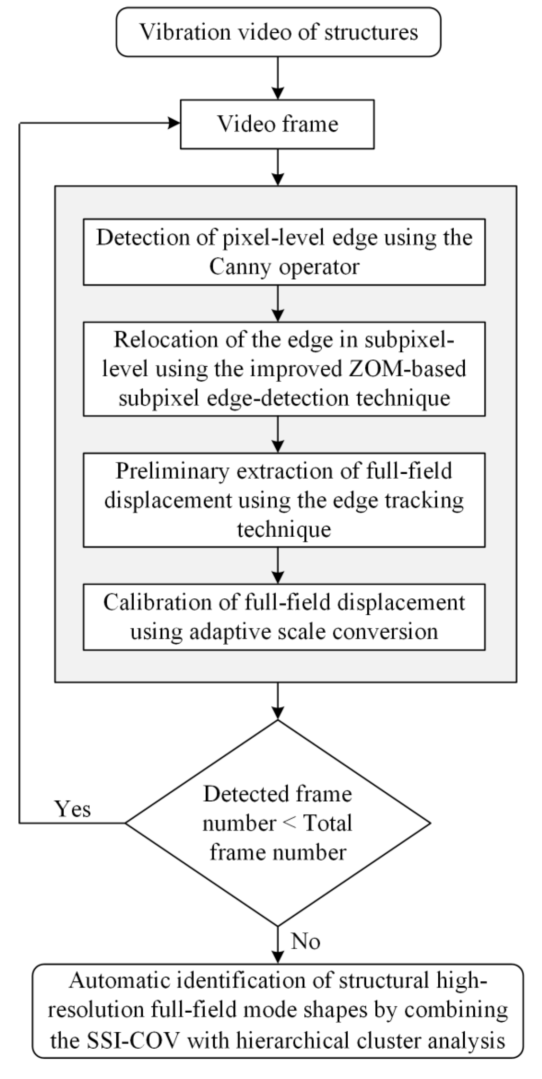
2. Theory and Methodology

The proposed full-field mode shapes identification method based on the subpixel edge-detection and tracking techniques involves four main steps, as shown in Figure 1.

Step 1: Apply the Canny operator [29] on each frame of the structure vibration video to extract the pixel-level edges that are expressed in integer-type coordinates.

Step 2: Apply the improved ZOM-based subpixel edge-detection technique to relocate the subpixel-level edges that are expressed in real number-type coordinates.

Step 3: Apply the edge tracking technique on the dense subpixel edges to obtain the preliminary full-field displacement time history and subsequently calibrate the displacement using the proposed adaptive scale conversion method.

Step 4: Apply the SSI-COV and hierarchical cluster analysis on the full-field displacement time history to automatically identify the high-resolution mode shapes of structures. Each step is detailed in the following subsections.

2.1. Detection of Pixel-Level Edge

Edge detection is a basic technique in image processing for feature extraction. The popular pixel-level edge-detection methods are the Roberts [33], Sobel [34], and Canny algorithms. The Roberts algorithm is very sensitive to noise and produces weak responses for genuine edges, while the Sobel algorithm is less sensitive to noise but has a long computation time. However, the Canny algorithm performs better than all these operators in almost all scenarios [35]. Thus, it is used to acquire continuous dense pixel-level edge points, and it mainly includes the following steps: (1) preprocess the ROI in the image using the Gaussian filter as a smoothing technique for noise removal; (2) calculate the gradient direction and amplitude of all pixels of the ROI; (3) find the local maxima of gradient amplitudes for all the pixels of the ROI using the non-maximum suppression and set the gradient amplitudes of the remaining pixels to be zero; (4) set two thresholds, T₁ and T₂, to classify the pixels into three parts—the pixel with a gradient amplitude >T₂ is defined as an edge point, the pixel with gradient amplitude <T₁ is defined as a non-edge point, and the pixel with a gradient amplitude between T₁ and T₂ is retained when adjacent to the edge points.

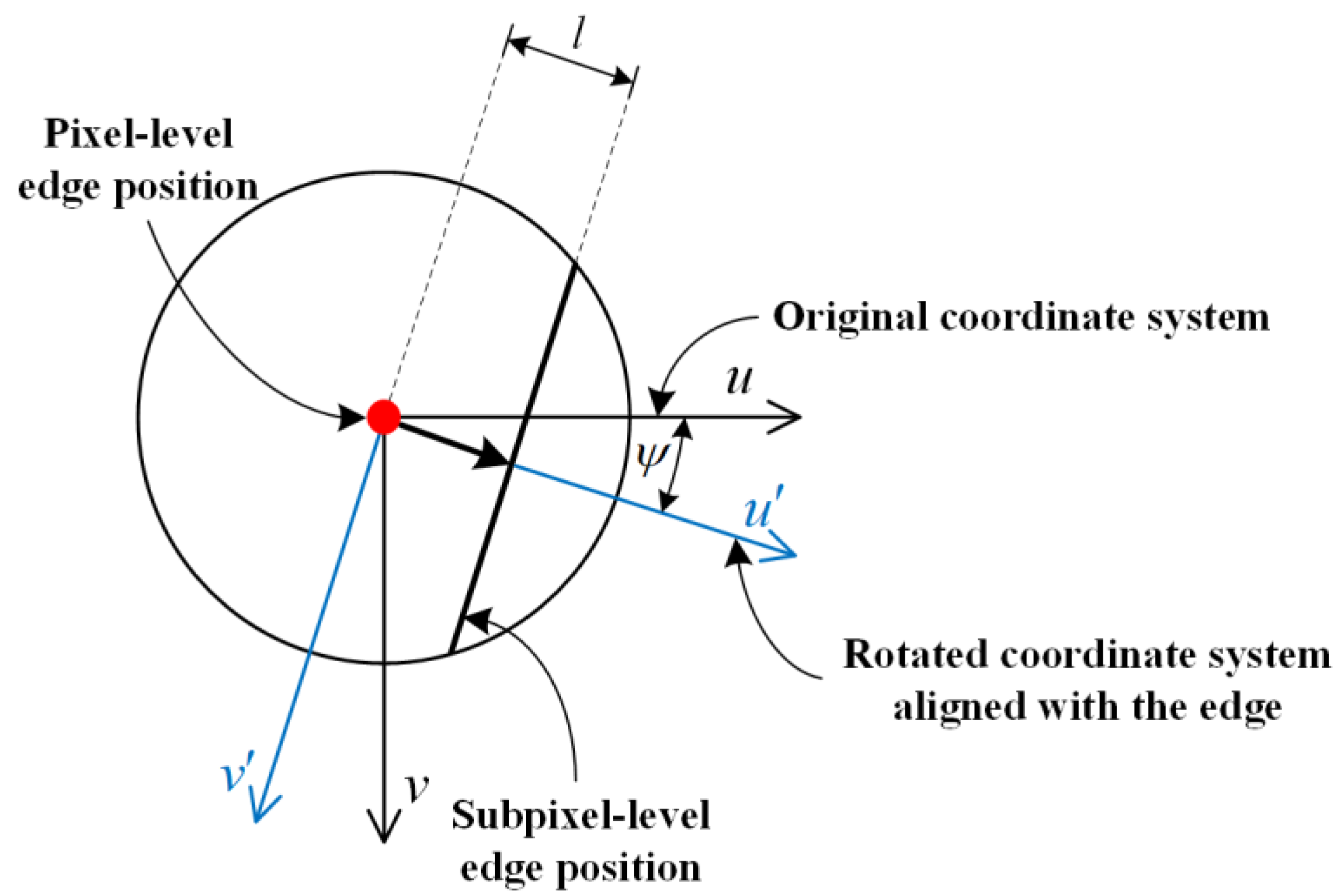
2.2. Relocation of the Edge in Subpixel-Level

The pixel-level edge-detection algorithms in the above step can only provide the location of the edge point at the pixel level, i.e., the coordinates of the edge points are integer pixels, which is not precise enough for the case with subtle vibrations. Thus, subpixel edge-detection techniques have been developed for precise edge localization, including four main categories, i.e., interpolation-based [36,37], fitting-based [38,39], moment-based [30,31,40,41,42,43,44], and the partial area effect (PAE) method [45]. Among them, the moment-based method is not sensitive to noise and is widely used. Hence, the subpixel edge-detection method based on the improved ZOM is adopted herein for relocating more precise edges, as elaborated below.

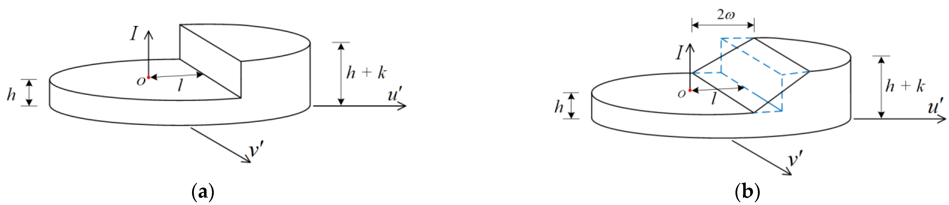
2.2.1. Improvement of the Edge Model

Most existing ZOM-based edge-detection methods adopt the simple step function as the edge model, assuming that the gray values at the edge change abruptly as seen in Figure 2a. In the figure, $v^{\prime }$ is the axis parallel to the edge, $u^{\prime }$ is the axis perpendicular to the edge, and I represents the pixel intensity. However, the intensity at the edge changes gradually in real images. Therefore, the linear ramp edge model has been developed for the intensity profile across an edge [31], as shown in Figure 2b, where l is the distance from the center to the ideal edge.

The ideal edge spread function (ESF) for the pixel intensity in a unit circle is expressed as

$$I(u^{\prime })=h+\frac{k}{2}\left[1+erf(\frac{u^{\prime }-l}{\sigma \sqrt{2}})\right],$$

(1)

where $\sigma$ controls the edge width, h represents the background intensity, and k is the step height.

After introducing the linear ramp edge model, the ESF in a unit circle can be expressed as a piecewise function as

$$I(u^{\prime })=\left\{\begin{array}{c}h\\ h+k\left[u^{\prime }-(l-\omega )\right]/(2\omega )\\ h+k\end{array}\right. \begin{array}{c}{u}^{\prime }\le l-\omega \\ l-\omega <u^{\prime }<l+\omega \\ u^{\prime }\ge l+\omega \end{array},$$

(2)

where $2\omega$ is the edge width. The function is approximate to the Gaussian ESF when $\omega =1.66\sigma$.

2.2.2. ZOM-Based Edge Location Calculation

After improving the edge model, the ZOM-based method is used to calculate the subpixel-level coordinates of the edges, as detailed in Ghosal and Mehrotra [30]. The Zernike moment of order n and repetition m for the 2D intensity function $f(u,v)$ is defined as

$$Z_{nm}=\frac{n+1}{\pi }{\displaystyle {\iint }_{u^2+v^2\le 1}f(u,v)T_{nm}(r,\theta )dudv}=\frac{n+1}{\pi }{A}_{nm},$$

(3)

where $f(u,v)$ is the gray value of pixel $\left(u,v\right)$ in the unit circle, $T_{nm}(r,\theta )$ is the Zernike moment kernel function expressed in polar coordinates.

The edge coordinates are determined based on the rotation invariance of ZOM; that is, the modulus of ZOM remains the same before and after the rotation of the image, only the phase angle changes. When the image rotates with an angle $\psi$ as shown in Figure 3, the relationship between $A_{nm}$ and ${A^{\prime }}_{nm}$ can be obtained through the polar coordinate transformation as,

$${A^{\prime }}_{nm}=A_{nm}{e}^{-jm\psi },$$

(4)

where $j=\sqrt{-1}$, $A_{nm}$ is the Zernike moment of the pixels in the original $u-v$ coordinate system, and ${A^{\prime }}_{nm}$ is the Zernike moment of the pixels in the rotated $u^{\prime }-v^{\prime }$ coordinate system aligned with the edge.

According to the condition that the imaginary part of ${A^{\prime }}_{11}$ is equal to zero, i.e., $\mathrm{Im}[{A^{\prime }}_{11}]=0$ [30], the edge orientation can be calculated in combination with Equation (4) as

$$\psi ={\tan }^{-1}(\frac{\mathrm{Im}\left[A_{11}\right]}{\mathrm{Re}\left[A_{11}\right]}),$$

(5)

where $\mathrm{Im}[A_{11}]$ is the imaginary part of $A_{11}$, and $\mathrm{Re}[A_{11}]$ is the real part of $A_{11}$. It is seen that only one Zernike moment $A_{11}$ is required to calculate the edge orientation. Meanwhile, the distance of the edge to the center can be obtained as

$$l=\left[1-{\omega }^2-\sqrt{{\left({\omega }^2-1\right)}^2-2{\omega }^2{A}_{20}/{A^{\prime }}_{11}}\right]/{\omega }^2,$$

(6)

Subsequently, the coordinate of the edge point in subpixel-level is determined as

$$\left[\begin{array}{c}u\\ v\end{array}\right]=l\left[\begin{array}{c}\cos (\psi )\\ \sin (\psi )\end{array}\right],$$

(7)

Two edge images generated by software and processed with Gaussian blurring, i.e., straight edge and curved edge, as illustrated in Figure 4, were used to compare the performance of the pixel-level and subpixel-level edge-detection algorithms. The pixel-level edge points extracted by the Canny operator and the subpixel-level edge points extracted by the improved ZOM-based method are shown in Figure 4, which shows that the subpixel-level edges are closer to the true edges than the pixel-level edges.

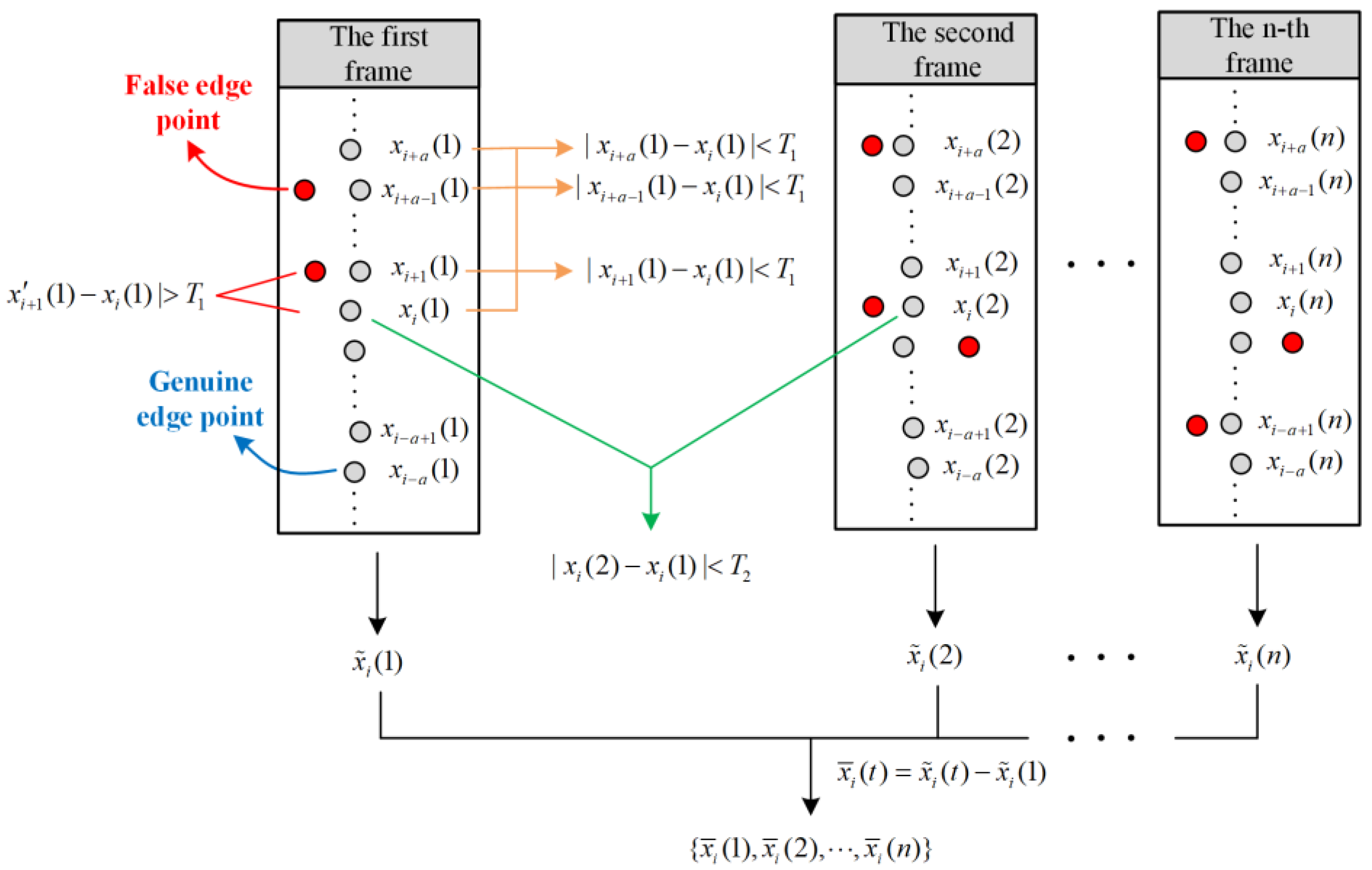
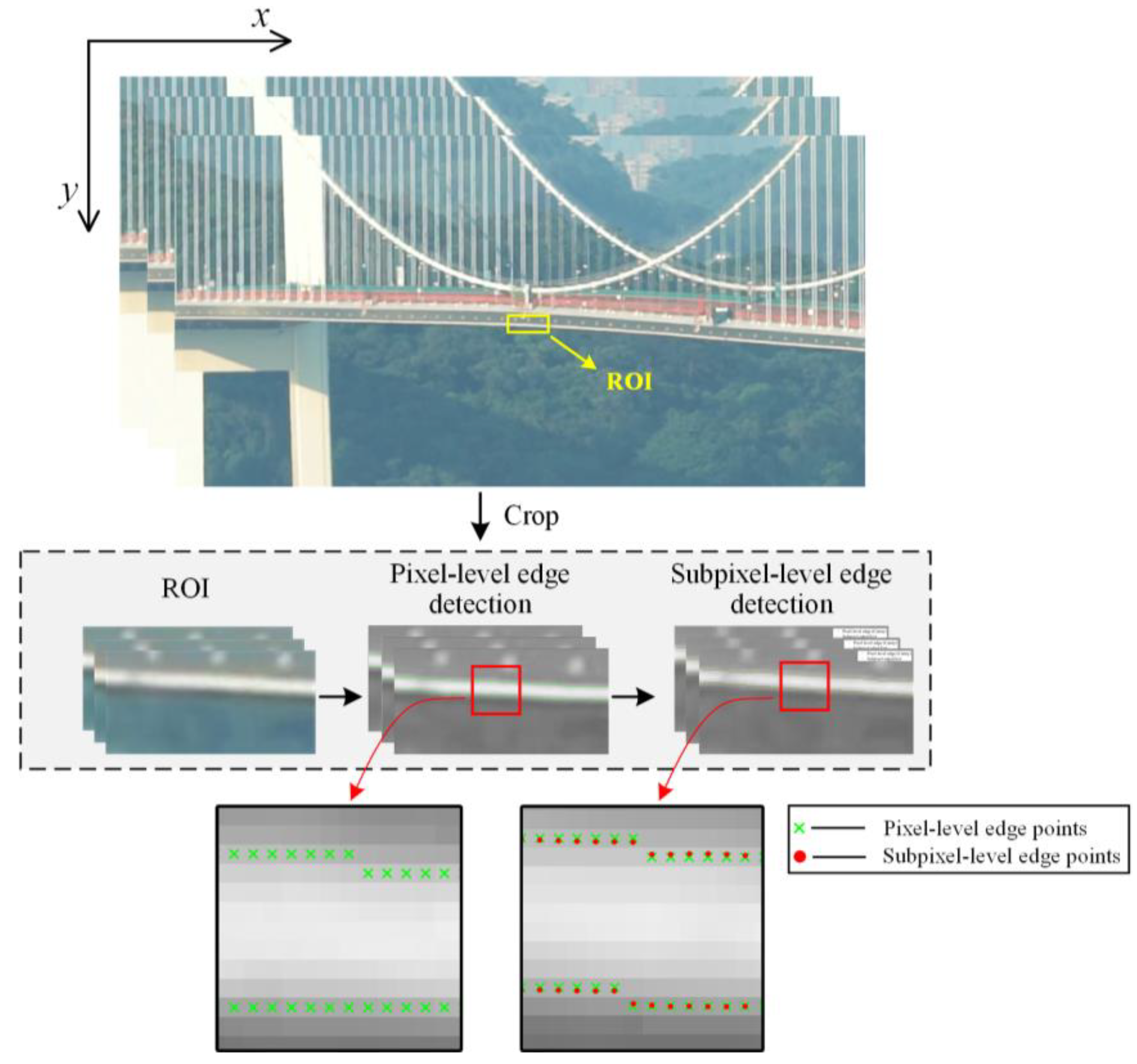
2.3. Extraction of Full-Field Displacement Time History

2.3.1. Displacement Extraction Based on Edge Tracking

The noise and other factors in the image may result in the detection of false edge points; that is, there could be more than one edge point at the same coordinates around the edge. As shown in Figure 5, the red points are false edge points. In order to eliminate those false edge points and obtain the genuine edges, a threshold T₁ is used to make the selection. For example, there are two points at the i+1th row in the first frame of Figure 5. The point with a horizontal distance to the reference point $x_i(1)$ larger than T₁ is treated as false edge point (i.e., the red point ${x^{\prime }}_{i+1}(1)$), and only one point with a distance smaller than T₁ is the genuine edge point (i.e., point $x_{i+1}(1)$).

Moreover, in order to improve the robustness of edge tracking, the average of 2a + 1 edge points is used to calculate the position of the edge point. For example, as for the edge point $x_i(1)$ in the first frame, all the edge points in the range of a, i.e., from point $x_{i-a}(1)$ to point $x_{i+a}(1)$, are used for averaging to calculate the coordinate of the point. For instance, if a = 1, three points are used for the average. Thus, the updated position of the edge point $x_i(1)$ is determined as

$${\tilde{x}}_i(1)=\frac{[x_{i-a}(1)+x_{i-a+1}(1)+\cdot \cdot \cdot +x_{i+a-1}(1)+x_{i+a}(1)]}{(2a+1)},$$

(8)

The position of the same edge point in each video frame is tracked to calculate the movement of the edge point, in such a way that the displacement of each edge point is obtained. In order to match the edge point in adjacent frames, a threshold of T₂ is used:

$$|x_i(t)-x_i(t-1)|<T_2,$$

(9)

where $x_i(t)$ and $x_i(t-1)$ are the horizontal coordinates in the frame t and $t-1$, respectively. The average process is repeated for each frame to calculate the updated position.

After the updated positions of the edge point in all frames are obtained, the horizontal movement of the edge point in the t-th frame relative to the first frame is calculated as

$${\overline{x}}_i(t)={\tilde{x}}_i(t)-{\tilde{x}}_i(1),$$

(10)

The time history of point i can be obtained as $\{{\overline{x}}_i(1),{\overline{x}}_i(2),\cdot \cdot \cdot ,{\overline{x}}_i(n)\}$, where n is the total number of video frames, as shown in Figure 5. By applying the same procedure on all the edge points, the full-field displacement time history of the structure edge can then be obtained.

2.3.2. Displacement Calibration Based on Adaptive Scale Conversion

For larger structures such as long-span bridges, if the camera is set at a long distance to the bridge and the shooting range includes the entire bridge, different positions of the bridge will have different scale factors due to the effects of camera distortion and shooting angle. Some studies ignore this effect by assuming that the optical axis of the camera is perpendicular to the plane of structure vibration, while some studies consider this effect through camera calibration by mounting a target on the structural surface. Herein, this study presents the adaptive-scale conversion method to calibrate the displacement. The principle is that the physical width of the measured structure remains constant, which is used as a base to calculate the scale factor at each position, as detailed below.

Choose a section as the reference position with the pixel width $l_0(t)$. According to the assumption that the physical widths of both positions are equal, the scale conversion factor at position i can be calculated as

$$l_0(t)=\left|{\tilde{y}}_0^u(t)-{\tilde{y}}_0^d(t)\right|,$$

(11)

$$l_i(t)=\left|{\tilde{y}}_i^u(t)-{\tilde{y}}_i^d(t)\right|,$$

(12)

$$k_i(t)=\frac{l_0(t)}{l_i(t)},$$

(13)

where ${\tilde{y}}_0^u(t)$ and ${\tilde{y}}_0^d(t)$ are the coordinates of the upper edge point and lower edge point at the reference position, while ${\tilde{y}}_i^u(t)$ and ${\tilde{y}}_i^d(t)$ are the coordinates of the upper edge point and lower edge point at the calibrating position i, respectively, as shown in Figure 6. $k_i(t)$ is the scale conversion factor of position i, and the displacement of all the points at position i, ${\overline{y}}_i{}^{\prime }(t)$, is calibrated by multiplying the original displacement ${\overline{y}}_i(t)$ with the scale conversion factor as follows:

$${{\overline{y}}^{\prime }}_i(t)=k_i(t)\cdot {\overline{y}}_i(t),$$

(14)

It is noteworthy that the displacement obtained here is the pixel displacement and is only used to identify the natural frequencies and mode shapes of structures. Therefore, it is not necessary to obtain the physical displacement of the structure.

2.4. Identification of Full-Field Mode Shapes

The operational modal analysis (OMA) method [32] is applied on the displacement time history extracted from the above procedure to identify the full-field mode shapes of the structure. Firstly, the SSI-COV method is applied to the full-field displacement time history to determine the modal parameters that are represented in the stability diagram. Then, the hierarchical cluster analysis is used, which leads to the automatic identification of mode shapes from the stability diagram while eliminating the false modes. The details are as follows.

2.4.1. Extraction of Modal Parameters Using SSI-COV

The full-field displacement time history of the structure is first expressed as a Hankel matrix, based on which the covariance matrix is constructed by calculating the elements using Equation (15) as

$$X_i=\frac{1}{N-i}{\displaystyle \sum _{k=0}^{N-i-1}{x}_{k+i}\cdot x_k^T},$$

(15)

where $x_k$ is a vector with the sampled outputs at time instant k, N is the number of points of the time series, and superscript T means transpose. The covariance matrix is constructed as follows:

$$T_{1|i}=\left[\begin{array}{cccc}{X}_i& X_{i-1}& \cdot \cdot \cdot & X_1\\ X_{i+1}& X_i& \cdot \cdot \cdot & X_2\\ \cdot \cdot \cdot & \cdot \cdot \cdot & \cdot \cdot \cdot & \cdot \cdot \cdot \\ X_{2i-1}& X_{2i-2}& \cdot \cdot \cdot & X_i\end{array}\right],$$

(16)

The singular value decomposition is then applied to obtain the system matrix, and the modal parameters are calculated by the eigenvalue decomposition.

2.4.2. Automatic Identification of Physical Modes Using Hierarchical Cluster Analysis

The stability diagram is typically used with the SSI-COV technique to determine the modal parameters. However, it requires to manually distinguish the false modes from all the identified modes to obtain the real modes. Therefore, the hierarchical cluster analysis is adopted to improve the efficiency and to automatically identify the physical (real) modes. Each modal parameter is regarded as a cluster, and the distance between each cluster is calculated. The two clusters with the smallest inter-cluster distance are merged into a new cluster, and the distances between clusters are recalculated and the merge process is repeated until the distances between all clusters are larger than the preset threshold. The inter-cluster distance is calculated as

$$d(r,s)=\left|\frac{f_r-f_s}{f_s}\right|+\left(1-MA{C}_{r,s}\right),$$

(17)

where $f_r$ and $f_s$ are the natural frequencies of r-order and s-order, and $MA{C}_{r,s}$ represents the modal assurance criterion between the r-order and s-order mode shapes.

3. Verification with Cantilever Beam Vibration

A vibration video of a cantilever beam in the literature [28] was analyzed to verify the feasibility and effectiveness of the proposed framework. The beam is made of aluminum with a fixed base at the bottom and a free end on the top. The beam structure was horizontally excited with an impact hammer on the bottom, and a stationary camera with a pixel resolution of 1920 × 1080 was used to record the structure vibration at a frame rate of 480 frames per second. The processed video has a duration of 1.25 s and contains 600 frames with a pixel resolution of 384 × 216. More details are referred to the literature [28].

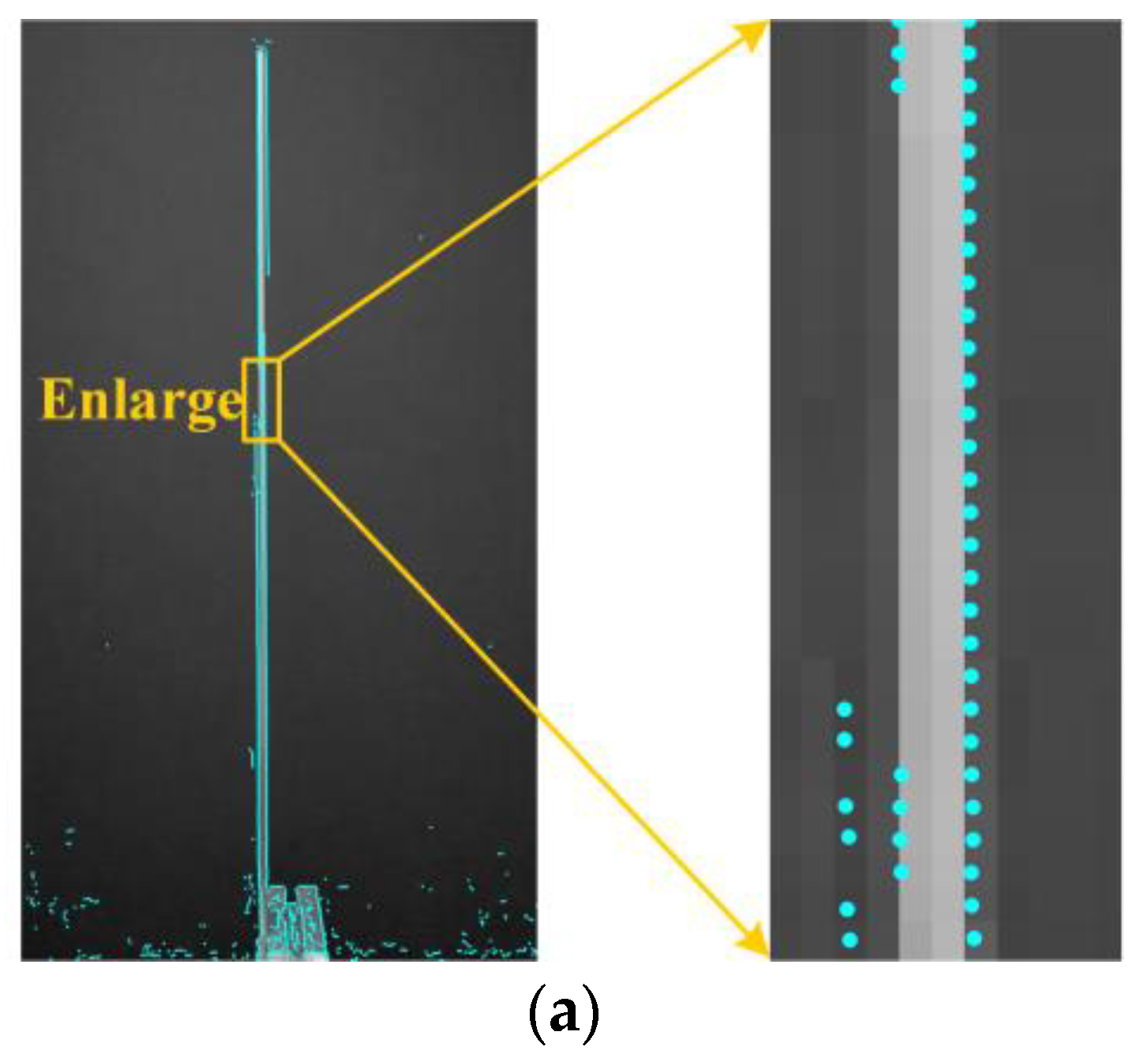
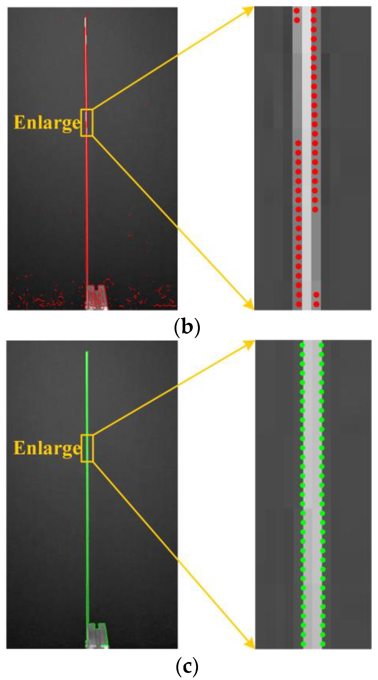
3.1. Results of Edges by Different Detection Algorithms

The proposed method uses the Canny operator to locate the rough pixel-level edge, and applies the ZOM-based algorithm to relocate the precise subpixel-level edge as shown in Figure 7. It can be seen that the subpixel-level edges are much closer to the true edge than pixel-level edges. That is, the ZOM-based subpixel algorithm significantly improves the accuracy of edge detection.

The performance of the proposed method was compared with the other two methods, i.e., the PAE-based algorithm and the method proposed by Christian [31] combining the Sobel operator with the ZOM-based algorithm, as shown in Figure 8. As can be seen in Figure 8a, many edge points are missing on the top part of the beam, and the method from the literature detected a lot of noise edge points at the bottom, while the result of the PAE-base method shown in Figure 8b is slighter better but still with a few missing edge points and many noise points. In contrast, the proposed method has detected a very complete edge and has almost no noise point as shown in Figure 8c. This indicates that the proposed method has very good performance in edge detection.

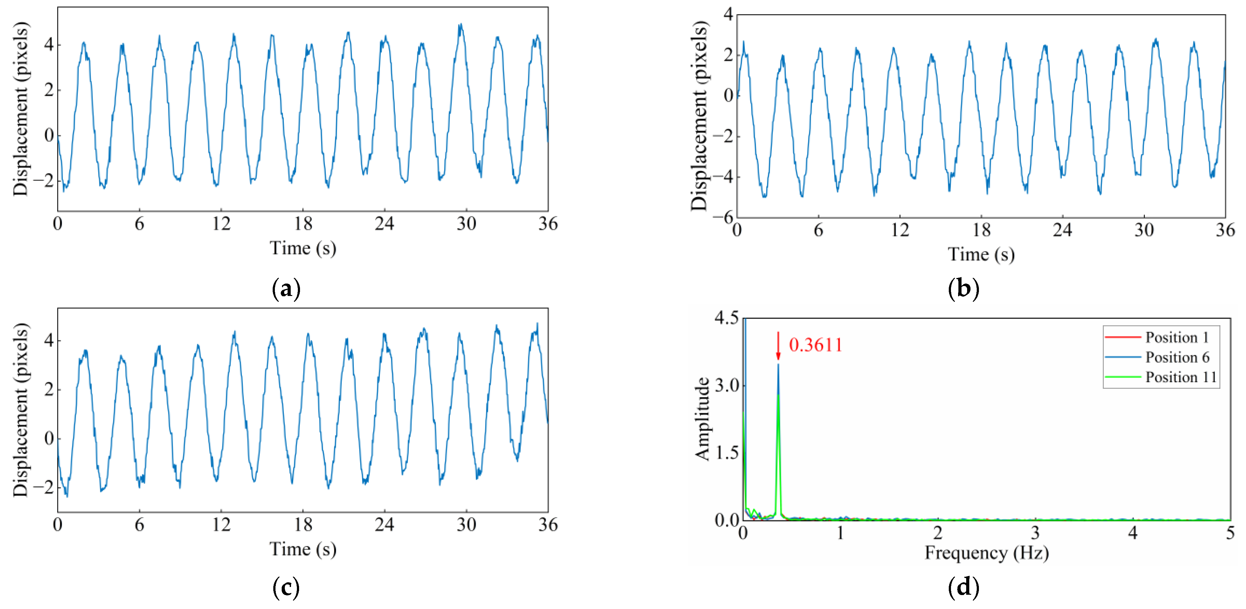
3.2. Results of Displacement Time History

The displacement time history of the beam can be extracted by tracking the movement of the detected edge points in all the video frames. Figure 9 illustrates the displacement time histories of the tracked edge shown in Figure 7 using the Canny operator and the above three subpixel edge-detection methods. As can be observed in Figure 9a, the displacement by the Canny operator contains many horizontal segments, implying that the displacement difference less than one pixel cannot be detected, which results in low accuracy of the displacement identification, especially for the cases with small vibration amplitudes. Figure 9b–d show the displacement time histories from the edges detected by the three subpixel algorithms, i.e., the algorithm in the literature [31], the PAE-based algorithm, and the proposed algorithm. By comparison, it is seen that the result of the proposed algorithm shows a good periodic pattern and is much better than the other two algorithms.

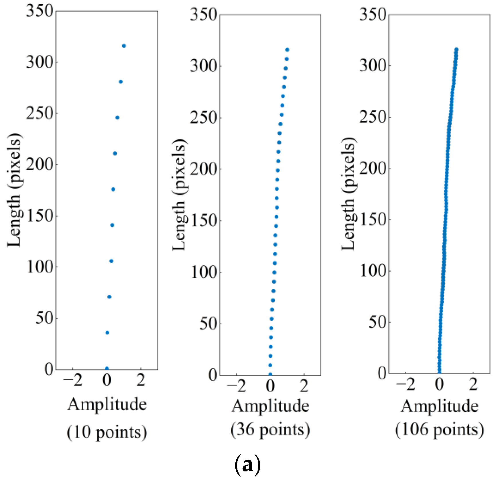
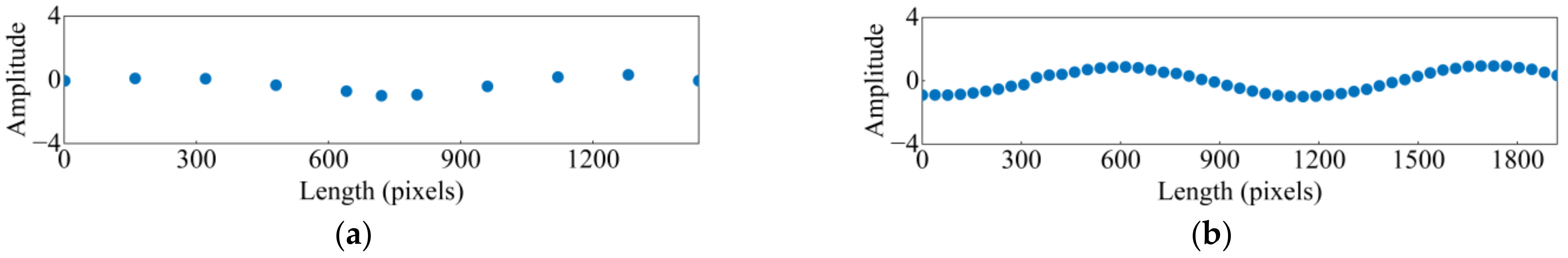
3.3. Results of Frequencies and Full-Field Mode Shapes

The fast Fourier transform (FFT) was applied to the displacement time history and the frequency spectra were obtained, as illustrated in Figure 10 (according to the Nyquist–Shannon sampling theorem, the maximum horizontal coordinate value is set to half of the camera frame rate, i.e., 240). It is apparent in Figure 10a that only the first bending vibration frequency of the cantilever beam can be recognized, while the algorithm from the literature and the PAE-based algorithm can identify the first two bending vibration frequencies with some noise peaks in between. In contrast, the proposed method can clearly identify the first four bending vibration frequencies.

Table 1. Comparison of vibration frequencies of the cantilever beam (unit: Hz).

Mode Number	① Theoretical Values [46]	② Proposed Method	Error (%) |②-①|/①
1	7.59	7.5	1.19
2	47.57	47.34	0.48
3	133.18	133.6	0.32
4	219.96	226.4	2.93

compares the frequencies identified by the proposed method with the theoretical values [46], which shows that the errors are within 3%.

The full-field displacement time history of the ROI shown in Figure 7 was further extracted by the proposed method to establish a measurement matrix $D(X,T)$, where X represents the number of edges sampled and T is the data volume of each edge throughout the sampling period. Then, according to the assumption that the thickness of the cantilever beam is a constant, the matrix was calibrated using the adaptive scale coversion method. Furthermore, the SSI-COV method was applied to obtain the physical modes from the calibrated matrix. Different numbers of displacement time history were selected as input signals from the matrix $D(X,T)$ to obtain sparse and full-field 2D mode shapes as shown in Figure 11.

The mode shapes of the cantilever beam can be identified based on the time histories of all the edge points. In this case, 316 subpixel points were identified for the edge of the cantilever beam. Thus, the full-field mode shapes containing any points (with a maximum of 316 points) as required can be identified. The fourth-order bending mode shape of the cantilever beam is weak and difficult to identify due to the effects of the camera recording quality and environmental noise. Herein, the first three bending vibration mode shapes of the cantilever beam identified using 10, 36, and 106 points are demonstrated in Figure 11, which shows that more edge points are selected, the higher the resolution of the 2D mode shapes that can be identified. The results show that the proposed method is capable of identifying the high-resolution full-field mode shapes without installing artificial targets.

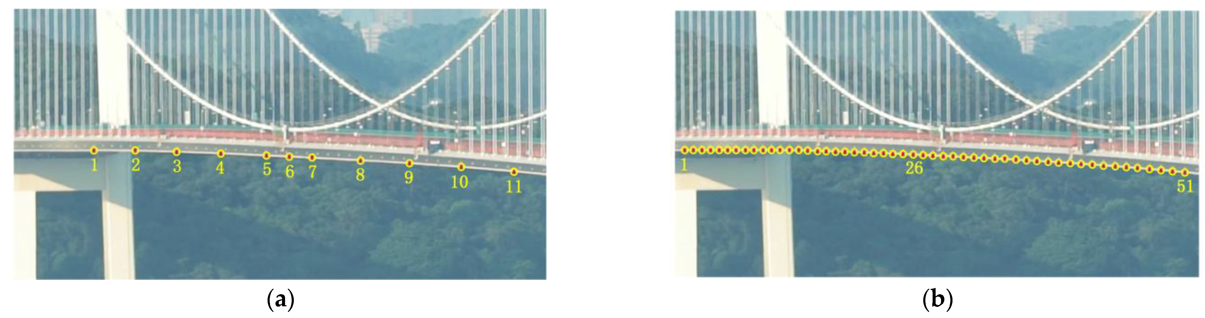
4. Application on a Real Bridge

The proposed method was applied for the modal identification of the Humen Bridge in China. A wind-induced vortex vibration occurred in 2020, and a video clip [47] was taken at a frame rate of 30 fps, containing 1080 frames with a pixel resolution of 1920 × 1080. Due to the large number of edge points of the bridge girder, only a few edge points depicted in Figure 12a,b were selected for measurement.

The lower edge of the bridge girder was extracted for the above positions. The position near the mid-span (i.e., ROI shown in Figure 13) was selected as an example for demonstration, as shown in Figure 13. The ROI was processed using the Canny operator to obtain the rough edge coordinates and the ZOM-based algorithm was used to precisely relocate the edge coordinates that were close to the true edge.

The vertical displacement time histories at positions 1, 6, and 11 in Figure 12a were extracted using the proposed method after obtaining the subpixel position of the bridge edge, as shown in Figure 14. The resonant frequency corresponding to the displacements of these three positions is 0.3611 Hz, which validates the repeatability of the proposed method. Compared with the measured frequency of Humen Bridge when it was built [48], it is found that the extracted frequency is in good agreement with the third-order frequency of vertical bending vibration, with an error of 2.06%. It is noted that for a long-span structure, the vibration can still be treated as small-amplitude vibration because its displacement is small with 2–4-pixel displacements in the image due to a long shooting distance.

Figure 15a,b show the identified 2D mode shapes of the bridge girder using 11 points and 51 points. From Figure 15a, it is difficult to determine which mode the mode shape belongs to, while it can be seen in Figure 15b that the identified mode shape is similar to the third-order mode shape of vertical bending vibration, which matches the frequency result. Thus, the proposed method can effectively determine the full-field mode shape of large-scale structures such as the Humen Bridge. It is noted that the public video used for this study has poor quality as a non-specialized test, and the proposed method can obtain more precise and complete mode shapes with higher resolution when conditions permit.

5. Conclusions

This study proposes a method of full-field mode shape identification based on the subpixel edge-detection and tracking techniques. The Canny operator and the improved ZOM-based subpixel edge-detection technique were adopted to detect the precise structure edges. The detected edge points were then tracked to obtain the displacement time histories, which were subsequently used to determine the full-field mode shapes of the structure. The proposed method was verified on an aluminum cantilever beam in the laboratory and the Humen Bridge in the field. The following conclusions are drawn:

(1)

The proposed method uses the Canny operator to locate the rough pixel-level edge and applies the ZOM-based algorithm to relocate the precise subpixel-level edge. The detected edge is very complete and close to the true edge, which shows a much better performance in edge detection compared to the methods in the literature.

(2)

The methods in the literature can only identify the first two bending vibration frequencies of the cantilever beam, while the proposed method can clearly identify the first four bending vibration frequencies, with errors of less than 3% of the theoretical values.

(3)

The results of the cantilever beam and the Humen Bridge confirm that the proposed method is capable of identifying high-resolution full-field mode shapes without installing artificial targets. A higher resolution of the mode shapes can be identified as more edge points are selected. The identified high-resolution mode shape of the Humen Bridge is helpful to the determination of modal characteristics.

However, this study has not considered the influence of complex environments in terms of, e.g., temperature, rain, fog, and atmospheric flow. The applicability under such conditions is the content of future research. In addition, since the actual displacements of the cantilever beam and Humen Bridge are not available, further tests will be conducted to verify the accuracy of the displacement identification using the laser displacement sensors.

References

1. Seo, J.; Hu, J.W.; Lee, J. Summary review of structural health monitoring applications for highway bridges. J. Perform. Constr. Facil. 2016, 30, 04015072. [Google Scholar] [CrossRef]
2. Ou, J.; Li, H. Structural health monitoring in mainland China: Review and future trends. Struct. Health Monit. 2010, 9, 219–231. [Google Scholar] [CrossRef]
3. Barbosh, M.; Singh, P.; Sadhu, A. Empirical mode decomposition and its variants: A review with applications in structural health monitoring. Smart Mater. Struct. 2020, 29, 093001. [Google Scholar] [CrossRef]
4. Cedolin, L. Stability of Structures: Elastic, Inelastic, Fracture and Damage Theories; World Scientific: Singapore, 2010. [Google Scholar] [CrossRef]
5. Xu, X.; Ren, Y.; Huang, Q.; Fan, Z.Y.; Tong, Z.J.; Chang, W.J.; Liu, B. Anomaly detection for large span bridges during operational phase using structural health monitoring data. Smart Mater. Struct. 2020, 29, 045029. [Google Scholar] [CrossRef]
6. Zhuang, Y.; Chen, W.; Jin, T.; Chen, B.; Zhang, H.; Zhang, W. A review of computer vision-based structural deformation monitoring in field environments. Sensors 2022, 22, 3789. [Google Scholar] [CrossRef] [PubMed]
7. Qian, H.; Wu, Y.; Zhu, R.; Zhang, D.; Jiang, D. Modal identification of ultralow-frequency flexible structures based on digital image correlation method. Appl. Sci. 2021, 12, 185. [Google Scholar] [CrossRef]
8. Peroš, J.; Paar, R.; Divić, V.; Kovačić, B. Fusion of laser scans and image data-rgb+d for structural health monitoring of engineering structures. Appl. Sci. 2022, 12, 11763. [Google Scholar] [CrossRef]
9. Kong, X.; Luo, K.; Deng, L.; Yi, J.X.; Yin, P.C.; Ji, W. Structural frequency identification based on broad-band phase-based motion magnification and computer vision. China Civ. Eng. J. 2022. [Google Scholar] [CrossRef]
10. Zhou, Y.; Cheng, Y.T. Non-contact structural displacement measurement based on digital image correlation method. J. Hunan Univ. 2021, 48, 1–9. [Google Scholar] [CrossRef]
11. Li, J.; Kong, X.; Yang, Y.; Yang, Z.; Hu, J. Optical flow based measurement of flow field in wave-structure interaction. Ocean Eng. 2022, 263, 112336. [Google Scholar] [CrossRef]
12. Feng, D.; Feng, M.Q.; Ozer, E.; Fukuda, Y. A vision-based sensor for noncontact structural displacement measurement. Sensors 2015, 15, 16557–16575. [Google Scholar] [CrossRef]
13. Feng, D.; Feng, M.Q. Experimental validation of cost-effective vision-based structural health monitoring. Mech. Syst. Sig. Process. 2017, 88, 199–211. [Google Scholar] [CrossRef]
14. Neri, P.; Paoli, A.; Razionale, A.V.; Santus, C. Low-speed cameras system for 3D-DIC vibration measurements in the kHz range. Mech. Syst. Sig. Process. 2022, 162, 108040. [Google Scholar] [CrossRef]
15. Horn, B.K.; Schunck, B.G. Determining optical flow. Artif. Intell. 1981, 17, 185–203. [Google Scholar] [CrossRef] [Green Version]
16. Caetano, E.; Silva, S.; Bateira, J. A vision system for vibration monitoring of civil engineering structures. Exp. Tech. 2011, 35, 74–82. [Google Scholar] [CrossRef]
17. Lucas, B.D.; Kanade, T. An iterative image registration technique with an application to stereo vision. In DARPA Image Understanding Workshop (IUW ′81); Carnegie Mellon University: Pittsburgh, PA, USA, 1981; Volume 81, pp. 674–679. [Google Scholar]
18. Guo, J. Dynamic displacement measurement of large-scale structures based on the Lucas-Kanade template tracking algorithm. Mech. Syst. Sig. Process. 2016, 66, 425–436. [Google Scholar] [CrossRef]
19. Cha, Y.J.; Chen, J.G.; Büyüköztürk, O. Output-only computer vision based damage detection using phase-based optical flow and unscented Kalman filters. Eng. Struct. 2017, 132, 300–313. [Google Scholar] [CrossRef]
20. Guo, J.; Wu, X.; Liu, J.; Wei, T.; Yang, X.; Yang, X.; He, B.; Zhang, W. Non-contact vibration sensor using deep learning and image processing. Measurement 2021, 183, 109823. [Google Scholar] [CrossRef]
21. Dong, C.Z.; Ye, X.W.; Jin, T. Identification of structural dynamic characteristics based on machine vision technology. Measurement 2018, 126, 405–416. [Google Scholar] [CrossRef]
22. Yoon, H.; Elanwar, H.; Choi, H.; Golparvar-Fard, M.; Spencer, B.F., Jr. Target-free approach for vision-based structural system identification using consumer-grade cameras. Struct. Control Health Monit. 2016, 23, 1405–1416. [Google Scholar] [CrossRef]
23. Dizaji, M.S.; Harris, D.K.; Alipour, M. Integrating visual sensing and structural identification using 3D-digital image correlation and topology optimization to detect and reconstruct the 3D geometry of structural damage. Struct. Health Monit. 2022, 21, 14759217211073505. [Google Scholar] [CrossRef]
24. Poozesh, P.; Sarrafi, A.; Mao, Z.; Avitabile, P.; Niezrecki, C. Feasibility of extracting operating shapes using phase-based motion magnification technique and stereo-photogrammetry. J. Sound Vib. 2017, 407, 350–366. [Google Scholar] [CrossRef]
25. Wadhwa, N.; Rubinstein, M.; Durand, F.; Freeman, W.T. Phase-based video motion processing. ACM Trans. Graph. 2013, 32, 1–10. [Google Scholar] [CrossRef] [Green Version]
26. Yu, L.; Pan, B. Single-camera high-speed stereo-digital image correlation for full-field vibration measurement. Mech. Syst. Sig. Process. 2017, 94, 374–383. [Google Scholar] [CrossRef]
27. Chen, J.G.; Wadhwa, N.; Cha, Y.J.; Durand, F.; Freeman, W.T.; Buyukozturk, O. Modal identification of simple structures with high-speed video using motion magnification. J. Sound Vib. 2015, 345, 58–71. [Google Scholar] [CrossRef]
28. Yang, Y.; Dorn, C.; Mancini, T.; Talken, Z.; Kenyon, G.; Farrar, C.; Mascareñas, D. Blind identification of full-field vibration modes from video measurements with phase-based video motion magnification. Mech. Syst. Sig. Process. 2017, 85, 567–590. [Google Scholar] [CrossRef]
29. Canny, J. A computational approach to edge detection. IEEE Trans. Pattern Anal. Mach. Intell. 1986, PAMI-8, 679–698. [Google Scholar] [CrossRef]
30. Ghosal, S.; Mehrotra, R. Orthogonal moment operators for subpixel edge detection. Pattern Recognit. 1993, 26, 295–306. [Google Scholar] [CrossRef]
31. Christian, J.A. Accurate planetary limb localization for image-based spacecraft navigation. J. Spacecr. Rocket. 2017, 54, 708–730. [Google Scholar] [CrossRef]
32. Magalhaes, F.; Cunha, A.; Caetano, E. Online automatic identification of the modal parameters of a long span arch bridge. Mech. Syst. Sig. Process. 2009, 23, 316–329. [Google Scholar] [CrossRef]
33. Roberts, L.G. Machine Perception of Three-dimensional Solids. Ph.D. Thesis, Massachusetts Institute of Technology, Cambridge, MA, USA, 1963. [Google Scholar]
34. Sobel, I.E. Camera Models and Machine Perception; Stanford University: Stanford, CA, USA, 1970. [Google Scholar]
35. Amer, G.M.H.; Abushaala, A.M. Edge detection methods. In Proceedings of the 2015 2nd World Symposium on Web Applications and Networking (IEEE), Sousse, Tunisia, 21–23 March 2015. [Google Scholar] [CrossRef]
36. Von, G.R.G.; Randall, G. A sub-pixel edge detector: An implementation of the canny/devernay algorithm. Image Process. Line 2017, 7, 347–372. [Google Scholar] [CrossRef] [Green Version]
37. Hermosilla, T.; Bermejo, E.; Balaguer, A.; Ruiz, L.A. Non-linear fourth-order image interpolation for subpixel edge detection and localization. Image Vis. Comput. 2008, 26, 1240–1248. [Google Scholar] [CrossRef]
38. Mortari, D.; de Dilectis, F.; Zanetti, R. Position estimation using the image derivative. Aerospace 2015, 2, 435–460. [Google Scholar] [CrossRef] [Green Version]
39. Ye, J.; Fu, G.; Poudel, U.P. High-accuracy edge detection with blurred edge model. Image Vis. Comput. 2005, 23, 453–467. [Google Scholar] [CrossRef]
40. Lyvers, E.P.; Mitchell, O.R.; Akey, M.L.; Reeves, A.P. Subpixel measurements using a moment-based edge operator. IEEE Trans. Pattern Anal. Mach. Intell. 1989, 11, 1293–1309. [Google Scholar] [CrossRef]
41. Qu, Y.; Cui, C.; Chen, S.; Li, J. A fast subpixel edge detection method using Sobel–Zernike moments operator. Image Vis. Comput. 2005, 23, 11–17. [Google Scholar] [CrossRef]
42. Tan, J.; Ao, L.; Cui, J.W.; Kang, W.J. Further improvement of edge location accuracy of charge-coupled-device laser autocollimators using orthogonal Fourier-Mellin moments. Opt. Eng. 2007, 46, 057007. [Google Scholar] [CrossRef]
43. Bin, T.J.; Lei, A.; Jiwen, C.; Wenjing, K.; Dandan, L. Subpixel edge location based on orthogonal Fourier–Mellin moments. Image Vis. Comput. 2008, 26, 563–569. [Google Scholar] [CrossRef]
44. Da, F.; Zhang, H. Sub-pixel edge detection based on an improved moment. Image Vis. Comput. 2010, 28, 1645–1658. [Google Scholar] [CrossRef]
45. Trujillo-Pino, A.; Krissian, K.; Alemán-Flores, M.; Santana-Cedrés, D. Accurate subpixel edge location based on partial area effect. Image Vis. Comput. 2013, 31, 72–90. [Google Scholar] [CrossRef]
46. Yang, Y.; Dorn, C. Affinity propagation clustering of full-field, high-spatial-dimensional measurements for robust output-only modal identification: A proof-of-concept study. J. Sound Vib. 2020, 483, 115473. [Google Scholar] [CrossRef]
47. B767–400ER. The Vibration Video of Humen Bridge in Dongguan During Traffic Suspension. Available online: https://www.bilibili.com/video/BV1Nt4y1178T (accessed on 20 January 2022).
48. Zhang, G.; Zhu, L. Test on vibration characteristics of Humen bridge. J. Tongji Univ. 1999, 2, 69–72. [Google Scholar]
Figure 1. Flowchart of full-field mode shapes identification of structures.
Applsci 13 00747 g001
Figure 2. Edge models: (a) step edge model; (b) linear ramp edge model.
Applsci 13 00747 g002
Figure 3. Image rotation.
Applsci 13 00747 g003
Figure 4. Comparison of pixel-level and subpixel-level edge detections: (a) straight edge; (b) curved edge.
Applsci 13 00747 g004
Figure 5. Displacement extraction of edge point.
Applsci 13 00747 g005
Figure 6. Calibration of edge displacement.
Applsci 13 00747 g006
Figure 7. Edge points extraction of the cantilever beam.
Applsci 13 00747 g007
Figure 8. Comparison of edge-detection algorithms: (a) algorithm in reference [31]; (b) PAE-based algorithm; (c) proposed algorithm.
Applsci 13 00747 g008aApplsci 13 00747 g008b
Figure 9. Displacement time histories of the cantilever beam: (a) Canny operator; (b) algorithm in reference [31]; (c) PAE-based algorithm; (d) proposed algorithm.
Applsci 13 00747 g009
Figure 10. Identified frequencies of the cantilever beam: (a) Canny operator; (b) algorithm in reference [31]; (c) PAE-based algorithm; (d) proposed algorithm.
Applsci 13 00747 g010
Figure 11. Bending vibration mode shapes of cantilever beam: (a) the first mode shape; (b) the second mode shape; (c) the third mode shape.
Applsci 13 00747 g011aApplsci 13 00747 g011b
Figure 12. Selected positions for measurement: (a) 11 edge points; (b) 51 edge points.
Applsci 13 00747 g012
Figure 13. Edge point extraction of the bridge girder.
Applsci 13 00747 g013
Figure 14. Displacement time history and natural frequency of girder: (a) position 1; (b) position 6; (c) position 11; (d) natural frequency.
Applsci 13 00747 g014
Figure 15. Identified mode shapes of girder: (a) 11 points; (b) 51 points.
Applsci 13 00747 g015