Article

Progressive Formation of Retrogressive Landslide and the Lateral Length of Instability

1
School of Resources and Safety Engineering, Central South University, Changsha 410083, China
2
Hunan Provincial Communications Planning, Survey and Design Institute, Changsha 410200, China
3
School of Geosciences and Info-Physics, Central South University, Changsha 410083, China
4
School of Civil Engineering, Hunan University, Changsha 410082, China
*
Authors to whom correspondence should be addressed.
Appl. Sci. 2023, 13(2), 799; https://doi.org/10.3390/app13020799
Submission received: 7 December 2022 / Revised: 3 January 2023 / Accepted: 4 January 2023 / Published: 6 January 2023
(This article belongs to the Special Issue Advances in Failure Behavior of Rocks)

Abstract

:
Retrogressive landslide is caused by the lower rock mass sliding, so that the upper part loses support, is deformed, and starts to slide. In the process of highway construction, the incised slope often leads to retrogressive landslide, and the determination of the damage range of retrogressive landslide is of great significance for the control of the slope. Taking a highway retrogressive landslide in Hunan Province as the research object, the particle flow discrete element is used to numerically simulate the entire failure process of the slope. According to the complex geological conditions of the slope, the rock mass of each part of the slope model is divided, the displacement of key parts of the landslide is monitored, the whole failure process of the retrogressive landslide is simulated, and the lateral length of traction instability is calculated through the stability theory of the sliding pull-crack failure slope. The research shows that the incised slope is the root cause of the retrogressive landslide, and the rainfall is the direct cause. When the retrogressive landslide is treated in engineering practice, the lateral length of traction instability can be obtained according to the stability theory of the sliding pull-crack failure slope, to realize the accurate judgment of the traction failure range of the sliding body.

1. Introduction

Deformation types of landslides generally include retrogressive landslide, load-caused landslide, and complex landslide [1,2]. Among them, retrogressive landslide is a process of backward progressive failure [3,4,5]. Due to slope erosion, or artificial slope cutting, the slope surface is deformed and unstable, and the lower rock mass first slides, and then gradually forms cracks from bottom to top [6,7]. With the development of deformation, the rock mass on the upper part of the slope loses support and slips [8]. Retrogressive landslides mostly occur in sloped areas composed of sedimentary layers, fault zones, weathering zones, and weak interlayers of rock and soil. The main sliding bodies are unconsolidated layers, weak interlayers, or ancient landslides, creep bodies, etc. [9,10,11]. When building expressways in mountainous areas, many sections of the road are constructed by removing the foot of the slope. Due to the man-made destruction of the foot of the slope, retrogressive landslides are easy to occur under the action of long-term natural forces (gravity forces). As a geological hazard, retrogressive landslide has the characteristics of wide distribution, high frequency, and great harm, which poses a major threat to engineering construction and people’s property safety [12,13,14]. Many scholars have done a lot of research work on retrogressive landslide [15,16,17]. Lin et al. [18] proposed a simplified numerical method for the prediction of rainfall-induced retrogressive landslides, which can effectively reduce the harm caused by retrogressive landslides caused by rainfall. Marko et al. [19] investigated the Audru landslide in detail and studied the influence of various modeling parameters on the overall slope stability. Lin et al. [20] carried out slope model experiments by filling an experimental flume with unsaturated fine sand and an artificial rainfall simulator and summarized the mechanism of rainfall-induced retrogressive landslides. At present, the research on retrogressive landslide generally uses indoor experiments or engineering cases to carry out qualitative analysis on its failure mode [21,22,23]. In order to control the retrogressive landslide and treat it [24,25,26], it is necessary to determine the instability range of the retrogressive landslide. As the retrogressive landslide is sliding from top to bottom, the slope will slip and crack to form numerous irregular slides. The reasons for the formation of these sliders and the range of the number of sliders need to be further studied. The length of the first sliding block formed by the retrogressive landslide is called the lateral length of traction instability, which is the distance between the bottom instability slip surface from the excavation surface to the trailing edge crack. In this paper, relying on the actual highway retrogressive landslide, the particle flow discrete element is used to analyze its failure mode, and the lateral length of traction instability is calculated through the stability theory of the sliding pull-crack failure slope, and the traction instability range of the retrogressive landslide is determined, and the influence of various rock parameters on the lateral length of traction instability is analyzed. The technical flow chart is shown in Figure 1.

2. Numerical Simulation of Landslide Failure Process

2.1. Geological Background

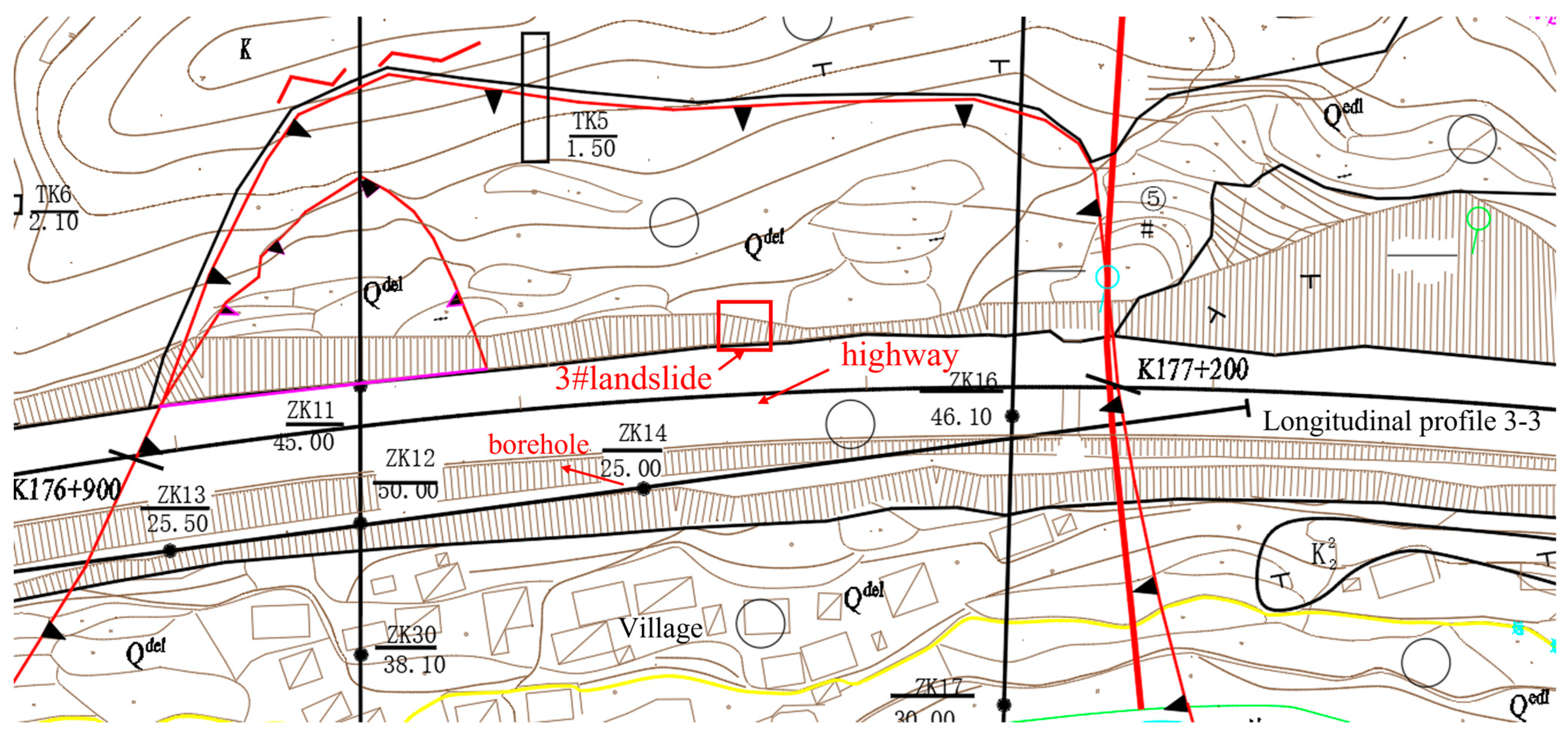
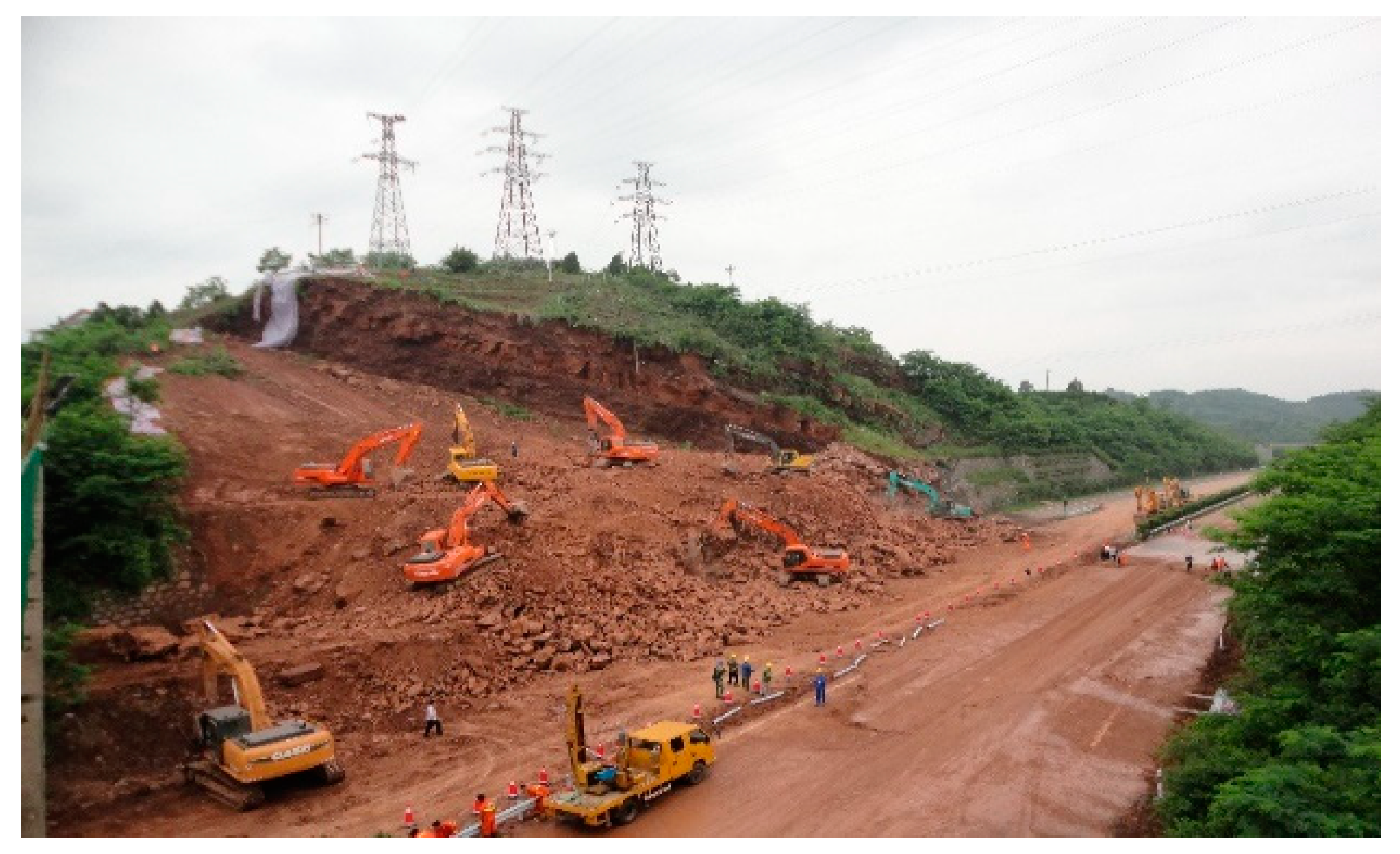
In May 2012, a rare continuous rainstorm occurred on the Luxi section of the Changde-Jishou Expressway in Hunan Province. A landslide occurred on the left upper slope of the K177 + 040~K177 + 115 section of the Changde-Jishou Expressway, as shown in Figure 2. A large amount of soil covered the highway, resulting in serious traffic jams in both directions, and major safety risks such as secondary landslides in the mountains and power cuts on high-voltage lines [27]. After geological investigation, it was found that the landslide was a retrogressive landslide [28,29], that is, the slope body showed a failure mode of segmented decline when sliding.
According to the 1:200,000 “Yeanling Regional Geological Survey Report” and geological maps, the survey area is in the western part of the Maying Depression Basin in Yeanling, mainly located in the southeast Hebei of the Luxe syncline. This area is in a mountainous terrain [30,31,32], with a maximum altitude of 188 m, a road design elevation ranging from 147.5 to 148.8 m, a maximum height difference of more than 40 m, and a natural slope between 25° and 30°. The vegetation distribution on the slope is relatively rich, mainly shrubs [33]. The angle between rock strata tendency and the direction of the highway is approximately 90 degrees. The panorama of the landslide is shown in Figure 3.
Mapping revealed the following lithologies:
(1)
Quaternary sediments: up to 0.5 m gray-brown soil, widely distributed on the hillside surface.
(2)
Late Cretaceous: medium-thick layered argillaceous sandstone, calcareous mudstone, and calcareous sandstone, etc. [34]. The calcareous sandstone and calcareous mudstone are alternately deposited, and there are weak interlayers of mud films with different thicknesses between the layers. The interlayer lithology is strongly weathered mudstone or plastic clay, and the properties are poor. A detailed summary is as follows:
Argillaceous sandstone: a thin-medium thick layer, with a huge thick layer of calcareous cementation; fully weathered rock mass is mostly hard plastic clay, with a small amount of strongly weathered rock mass locally, and the thickness is generally less than 0.5 m; strongly weathered rock mass is purplish red, steep inclination joint cracks are developed, the rock mass is broken, the rock quality is weak, and the thickness of this layer is generally less than 6.0 m; moderately weathered rock mass is purplish gray, purplish black, the rock mass is relatively complete, and the rock quality is relatively soft.
Calcareous sandstone: a thin-medium thick layered, calcareous cemented; fully weathered rock mass is mostly brown-gray, with a small number of strongly weathered rock blocks, and the layer thickness is less than 0.50 m; strongly weathered rock mass is brown-yellow and brown, and the rock mass is relatively broken and soft; moderately weathered rock mass is light gray-red, the rock mass is relatively complete, and the rock quality is relatively soft.
The stratigraphic lithology division is shown in Figure 4.

2.2. PFC Introduction

There are many numerical methods for rock mechanics analysis [35,36,37], among which the discrete element method is suitable for studying the dynamic characteristics of discontinuous media. The particle flow method is a quantitative evaluation method based on the framework of the discrete element model. Particle Flow Code (PFC) is a calculation software developed by Itasca Company in the United States, including PFC2D and PFC3D. It is particularly useful for simulating the operation and interaction of two-dimensional disks or three-dimensional spheroid aggregates of any shape and size [38]. The PFC model [39] simulates the movement and interaction of many finite-sized particles. The particles [40,41,42] are rigid bodies with finite mass that move independently of one another and can both translate and rotate. Particles interact at pair-wise contacts by means of an internal force and moment. Contact mechanics is embodied in particle-interaction laws that update the internal forces and moments. The time evolution of this system is computed via the distinct-element method, which provides an explicit dynamic solution to Newton’s laws of motion.
Thanks to its general design, PFC can be easily customized and applied to a very broad range of numerical investigations where the discrete nature of the systems is of interest. It has been successfully used by many academic institutions and private companies around the world for problems ranging from fundamental research on soil and rock behavior at the laboratory scale to slope stability [43,44,45] and rockfall hazard mitigation [46], hydraulic fracturing, rock-tool interactions, bulk flow, mixing, conveying and compaction of aggregates and powders, and blast furnace modeling, etc.

2.3. Meso-Calibration of Rock Materials

PFC differs from other methods in that the meso-parameters of the particle discrete element model cannot be directly derived from the mechanical parameters obtained from the physical test of rock materials [47,48,49]. For the meso-parameters of the rock material particle flow model, it is usually necessary to compare the macro-mechanical parameters (shear force parameters, elastic modulus, etc.) of the indoor physical test and the stress-strain relationship [50]. In the particle flow software PFC2D, the numerical tests used for the calibration of particle discrete element model parameters include a biaxial compression test, an uniaxial compression test, a direct shear test, and a Brazilian splitting test, etc. In the numerical simulation of retrogressive landslide, the meso-parameters of rock materials are determined mainly through a direct shear test. The matching results are shown in Table 1, Table 2, Table 3 and Table 4.

2.4. Landslide Model Establishment

The CAD slope profile obtained from site investigation is converted into a file format matching PFC, and imported into PFC2D, and modeled at the scale 1:1. Figure 5 is the CAD slope profile (model of the highway case).
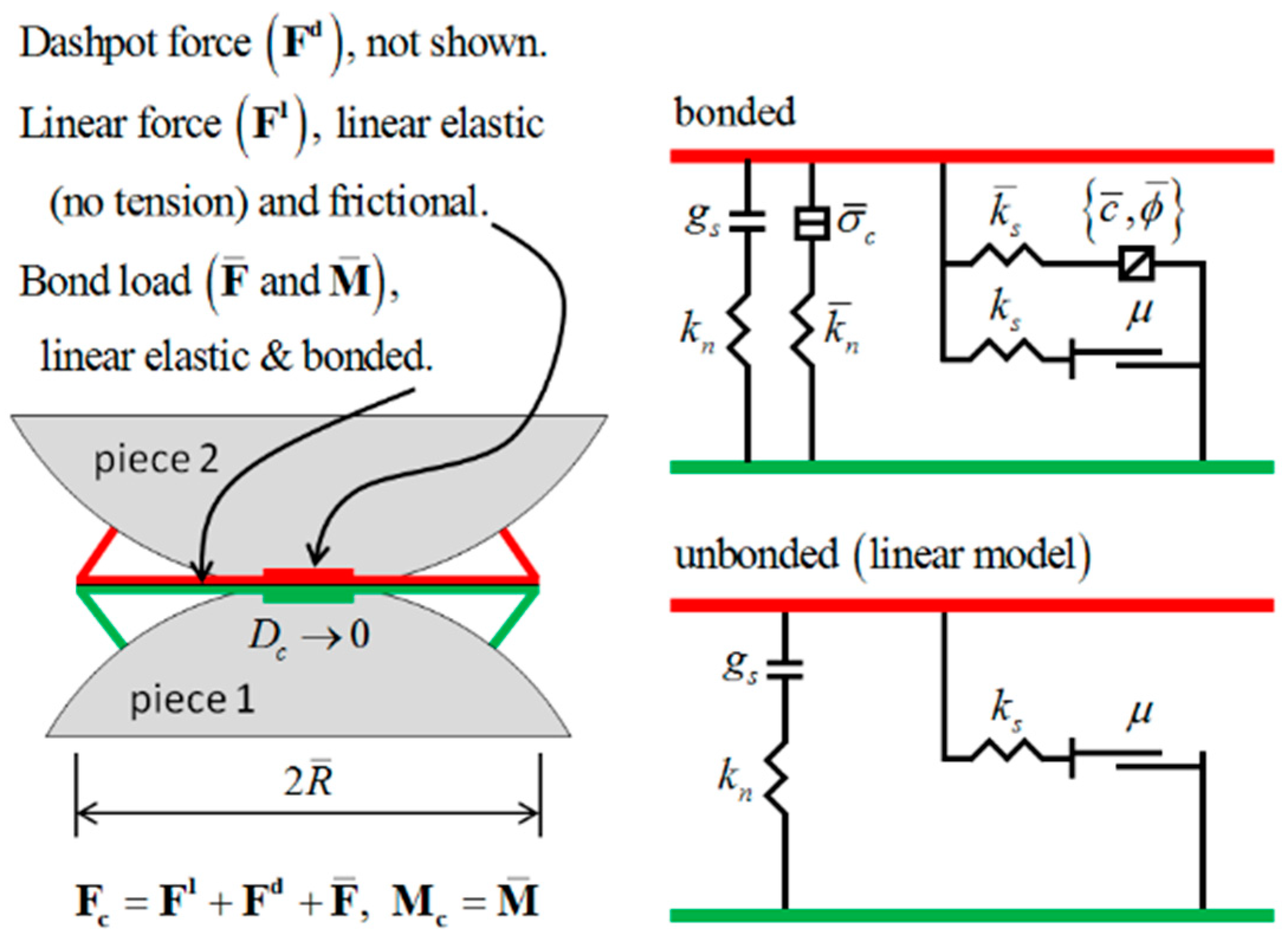
Wall elements in PFC2D have two functions: (a) to keep the shape of the model unchanged; (b) as a boundary condition. Walls in the slope model can be classified into two types according to the above functions: one is to fix the shape of the entire model, including a retaining wall, a highway, etc. The other is to limit the displacement of the boundary ball (which will be removed later). The contact model of PFC2D can be divided into: the Contact-Stiffness Model, the Slip Model, the Bond Model, and Alternative Models. The Parallel-Bond Model in the Bond Model is a commonly used contact model when simulating rock materials. As shown in Figure 6, the Parallel-Bond Model typically contains parallel-bond elements, wire spring elements, and dampers. Once the maximum normal or tangential stress on the bond exceeds the bond strength, the bond breaks off, and the Parallel-Bond Model after fracture is equivalent to the Linear Contact Model.
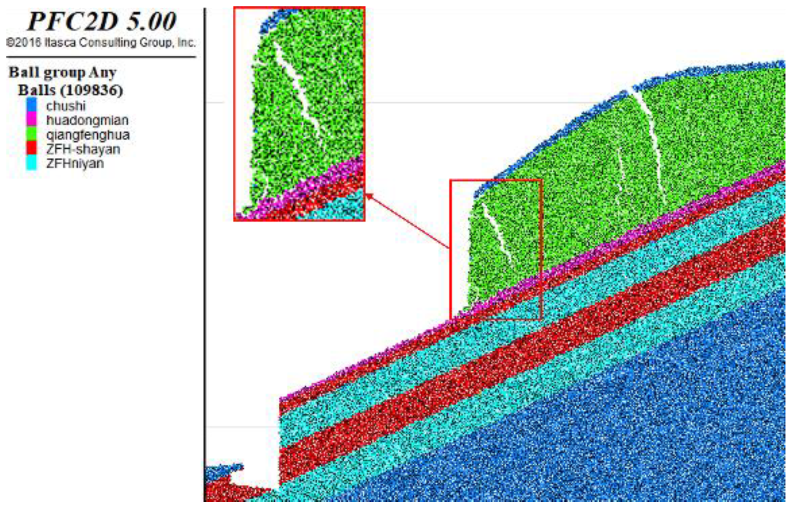
The meso-parameters of the obtained rock material are added to the model. At this point, the particles in the slope model begin to move due to their mechanical properties. It is necessary to reset the particle displacement and the contact force (moment) experienced by the particles to 0 to re-equilibrium the model, so as to reduce the initial influence of the model on the axial stress and strain calculation. The slope model is shown in Figure 7.
The slope model is 125 m long and 65 m high, the foot of the slope is 88°, the dip angle of bedding is 25°, and the total number of particles is 109,836.

2.5. Analysis of Landslide Failure Mode

The failure process is observed after the constraint wall is removed, gravity is added, and the model is run for 100,000 steps.
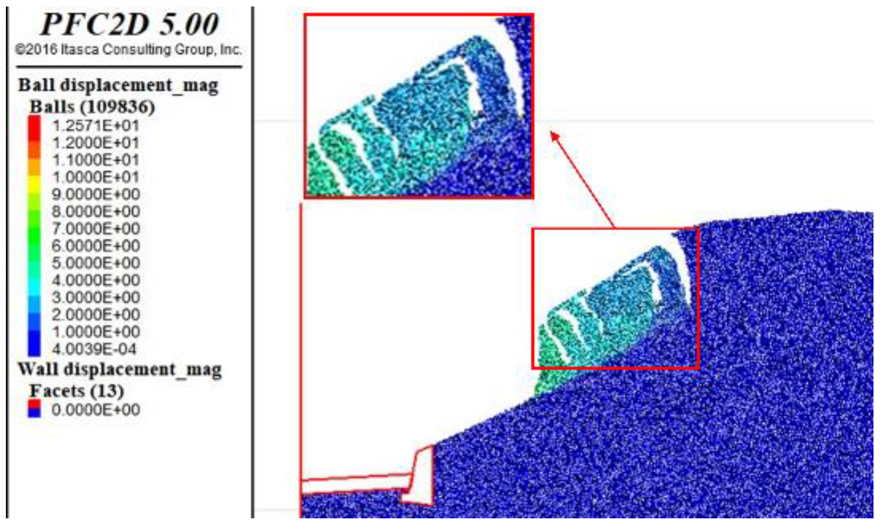
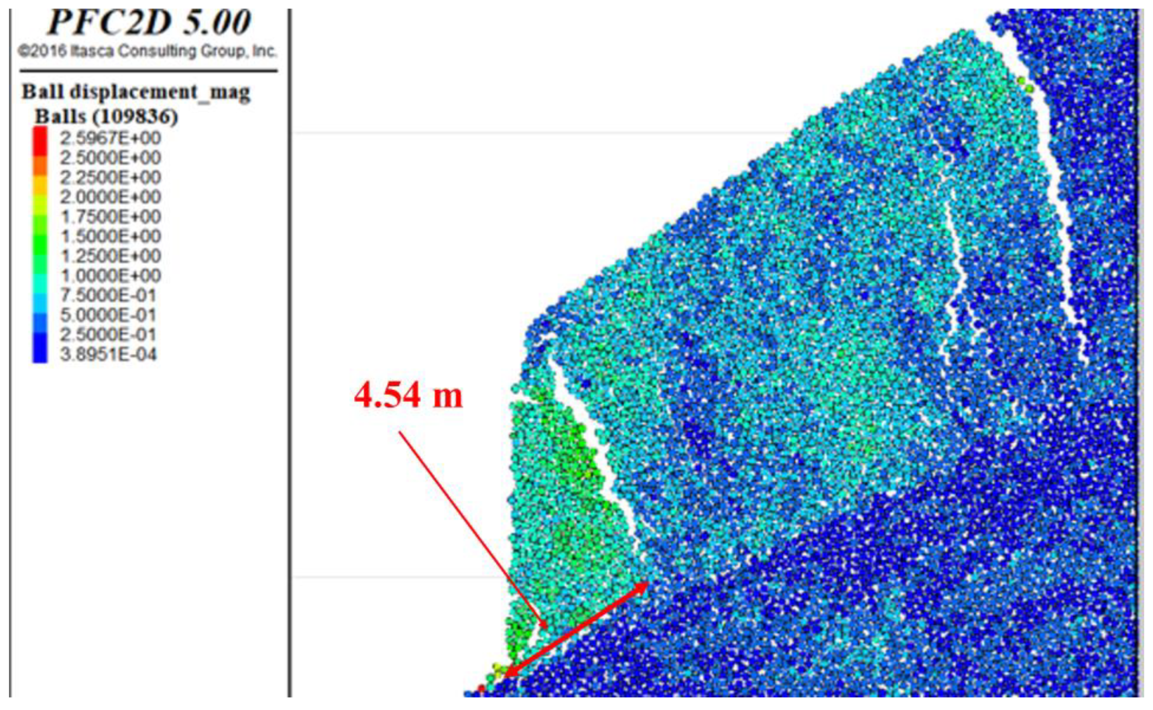
At 37,500 time-steps, the slope begins to break, as shown in Figure 8. From the grouping of particles in the model, it can be seen that the planting soil part on the upper part of the slope and the strongly weathered calcium argillaceous sandstone began to slide along the sliding surface, and two obvious tension cracks appeared. One appeared in front of the slope, about 4.54 m away from the foot of the slope, which was the first part to crack. The other appeared in the middle of the slope, and gradually expanded from the foot of the slope. The overall displacement and velocity of the slope are small, which is due to the artificial removal of the foot of the slope to form a free surface. Under the action of gravity, the slope body undergoes shear creep in the direction of the free surface.
PFC2D continues to run, resulting in Figure 9. At this point, damage occurs in the middle of the slope. With the increase of displacement, the middle part of the slope is pulled and cracked into several blocks, and five pull-crack cracks penetrate the front and middle part of the slope. The displacement of the slope gradually increases from top to bottom, and the maximum displacement of particles in the lower part of the slope reaches 12.57 m. At this time, the rock mass on the upper part of the slope has not slipped yet. It can be seen that the speed of particles in different parts is different, which is a ladder-shaped distribution. The front particles of the slope body have a fast speed, constantly dragging the rear particles, showing obvious displacement segmentation. This is because the lower part of the slope slides downward due to the failure of particle adhesion, causing the upper part of the particle to lose support and generate downward acceleration and kinetic energy, pushing the particles in the front of the slope to continue to slide forward. It can be seen that when the particle adhesion force is large, the rock mass will not fall completely apart when a landslide occurs, but rather slides down as a coherent block.
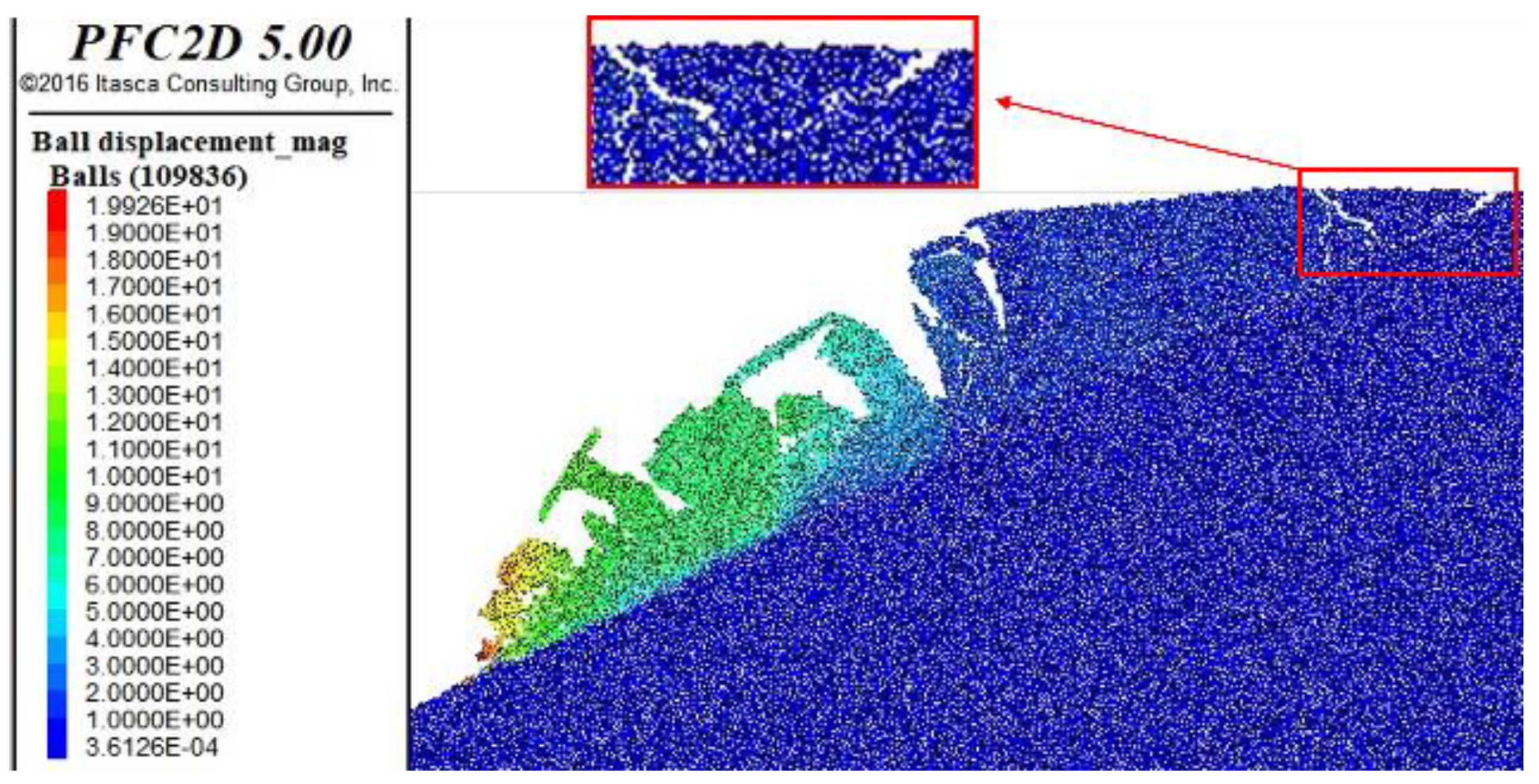
In later time steps the upper part of the slope begins to destabilize, as shown in Figure 10. At time-step 388 × 10³ the displacement is further increased, and the central rock mass was completely pulled off. At this time, a new crack appeared in the upper rock mass, but it has not yet been pulled into multiple blocks. At the top of the rock mass a longer crack appears along the sliding surface and increases in thickness. At this time, the maximum displacement of rock particles is 19.926 m, and the sliding zone has basically cut through with the overlying rock mass sliding along the underlying soft rock layer. Under the self-weight stress, it fills the empty surface and is continuously piled up at the foot of the slope.
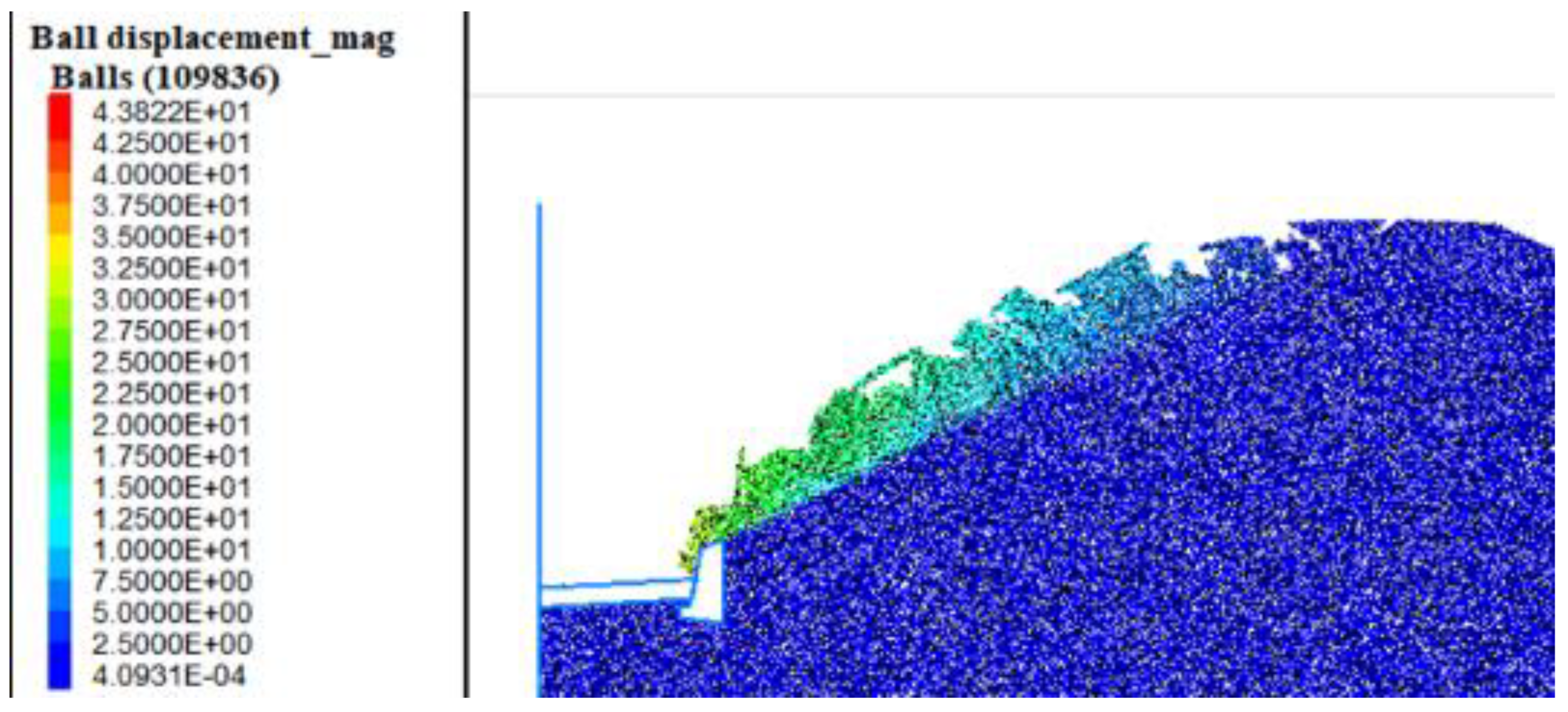
The numerical simulation of the slope was completed, and Figure 11 was obtained. The slope has completely collapsed. The displacement of the upper particles is the largest, and the displacement of the lower particles is relatively small. This is due to the sliding of the rock mass at the front edge of the slope; shear failure occurs in the middle of the slope, the rock mass at the rear edge loses its support and slides downward, and the stress on the upper particles of the slope is greater than that of the lower particles, resulting in a significant change in the displacement of the upper particles of the slope. At this time, the rock mass at the front edge of the slide slides forward through the retaining wall to the model highway. At this time, the maximum displacement of the rock particles reached 43.822 m.
This research demonstrates that the particle flow method has good applicability to the simulation of the failure movement process of landslides. Due to the poor geological conditions, the incised slope is the fundamental cause of landslide. Under natural conditions, the slope composed of joints [51], cleavage, and weak interlayers in rock-soil has a higher safety factor and is in a higher equilibrium and stable state. When the foot of the slope is artificially incised, the shear stress and normal stress of the structural surface increase. The original “key block to resist sliding”, that is, the locking section, is destroyed or cut off, resulting in the gradual reduction of the average cohesion force on the structural surface. The original isolated and disordered instability areas no longer act alone but try to penetrate the potential sliding surface in an orderly sliding and expanding manner. Finally, when the sliding surface is completely penetrated, the sliding body quickly slides along the sliding surface towards the air-facing surface, and the slope is unstable and damaged as a whole, resulting in landslide disasters. Rainfall is the direct cause of landslide. Rainfall has an important influence on slope damage. From early April to late May, the total rainfall in the Luxi area reached 448 mm, and the rainfall reached a heavy rain state for 6 days. It can be considered that the rock and soil in the slope were saturated at this time, and the cohesion and internal friction angle were greatly reduced. Continuous rainfall caused rainwater to infiltrate into various joint cracks in the slope body from the surface cracks of the slope body, and continuously accumulated to form hydrostatic pressure [52,53]. The hydrostatic pressure forced the joints to further crack, making rainwater accumulate further, forming a vicious circle, and eventually causing landslides [54]. Rainfall also caused the weight of the sliding body to increase and further slip deformation along the sliding surface. Due to excavation, rainfall, and other reasons, the slip of the foot of the slope often made the adjacent blocks lose part of the anti-sliding force, which led to stress concentration and softening [55]. Climatic conditions cause the slope to be destroyed, but the geological conditions of the slope are the root cause of the retrogressive landslide.

3. Determination of Lateral Length of Traction Instability and Analysis of Influencing Factors

3.1. Determination of Lateral Length of Traction Instability

During the construction of the slope, due to the effects of rainfall, the removal of lateral constraints, blasting [56], and other factors, the rock mass structure in the local area of the slope is destroyed, thereby reducing its mechanical index. The mechanical principle is complex, and it is very difficult to describe this process accurately and completely. Assuming that the bottom surface of the rock mass in layer i is a weak surface after the slope is excavated, the rock mass of the slope will slide along this bottom surface. For slopes whose excavation slope angle is greater than the dip angle of bedding, because of the removal of material by excavation, the failure mode of the slope may be a complete sliding failure along a certain level, or it may slide along certain levels. During the sliding process, some joints in the rock mass are pulled apart, showing gradual sliding failure from bottom to top. For the slope with the natural slope angle equal to the dip angle of bedding, the slope calculation model shown in Figure 12 is established. Let the dip angle of bedding be α and the excavation slope angle be β. The x-axis position of the coordinate system is taken as the bottom surface of the studied block and changes with the change of the studied block. The origin of the coordinate is located at the intersection of the bottom surface of the studied block and the excavation surface. Let the origin of the coordinates be Ai, C is a point on the excavation slope, and the intersection of the vertical line and the x-axis is Bi. E is the apex angle of the slope and let its x and y coordinate values be x0 and y0. F is any point on the bottom of the i-th layer. The distance from G to the origin of the coordinate system is L0. L0 is the width of the weakening area of the mechanical parameter, that is, the length of the influence area of the incised slope is L0. L0 is related to factors such as construction methods, rock mass unloading, and weathering, and can be determined according to engineering experience.
From previous research, it can be seen that in the process of slope slip failure, the range of the part of the rock mass where the mechanical parameters of the rock mass decline are limited, generally near the empty surface of the slope. Second, in this area, the closer to the surface of the slope, the greater the magnitude of the decrease in the value of the mechanical parameters of the rock mass. The further away from the surface of the slope, the smaller the magnitude of the decrease in the value of the mechanical parameters of the rock mass, and the closer it is to the value in the natural state. It can be seen from Figure 12 that the mechanical parameters of point A are most affected, and the mechanical parameters of point G are not affected, which is natural. In order to calculate the lateral length of traction instability, three parameters need to be determined, namely friction coefficient, cohesion, and tensile strength. For point F, let fi be the friction coefficient of the bottom surface of the i-th layer, ci be the cohesion of the bottom surface of the i-th layer, and Sti be the equivalent tensile strength of the rock mass above the bottom surface of the i-th layer. The three mechanical parameters of point G are “Sri, fri and cri”, and point A are “Spi, fpi, and cpi”. Assuming that the influence of the incised slope on the mechanical parameters of rock mass decreases linearly, then the relationship between the distance x from point F to the origin of the coordinate system and the mechanical parameters of point F is:
f i = { k f i x + f r i f p i 0 x L 0 x > L 0 c i = { k c i x + c r i c p i 0 x L 0 x > L 0 S t i = { k s i x + S r i S p i 0 x L 0 x > L 0
In the formula, kfi, kci, and ksi are the corresponding coefficients defined as:
{ k f i = f p i f r i L 0 k c i = c p i c r i L 0 k s i = S p i S r i L 0
If the first sliding part is the front triangle, the following relationships can be derived for the triangle AiBiC from simple goniometry:
| A i B i | = x | B i C | = x tan ( β α )
Let WAiBiC be the weight of triangle AiBiC,
W A i B i C = 1 2 γ ¯ | A i B i | · | B i C |
where γ is the average bulk density of overlying strata on layer I in the formula.
On the pull-crack surface BiC, let Fsi be the tensile force of the tensile strength of the rock mass to the triangle AiBiC.
F s i = | B i C | S t i
On the sliding surface AiBi, Fqi is the tensile force of rock mass on the triangle AiBiC. Fqi is mainly composed of a friction coefficient and cohesion on the sliding surface.
F q i = W A i B i C cos α · f ¯ i + x · c ¯ i
where f ¯ i , c ¯ i are the average friction coefficient and cohesion on the sliding surface.
Let FDi be the sliding force of the triangle AiBiC:
F D i = W A i B i C · sin α
Add Equations (4) and (5) to obtain the total anti-sliding force of block AiBiC, denoted as FRi.
F R i = F s i + F q i = | B i C | S t i + W A i B i C cos α · f ¯ i + x · c ¯ i
If FDi > FRi, the landslide has occurred. If FDi < FRi, the landslide will not occur. If:
F R i F D i = 0
The slope is in the limit equilibrium state, about to slide but not yet. The unknown x in the equation at this time is the lateral length L of the traction instability, denoted as LHi. Substituting Equations (1)–(7) into Equation (8) gives a univariate quadratic equation, which can be solved:
L H i = { A 12 + A 12 2 4 A 11 A 13 2 A 11 ( L H i L 0 ) A 22 + A 22 2 4 A 21 A 23 2 A 21 ( L H i > L 0 )
In the formula:
{ A 11 = 1 4 γ ¯ tan ( β α ) cos α · k f i A 12 = 1 2 tan ( β α ) · ( 2 k s i + γ ¯ cos α · f r i γ ¯ sin α ) + 1 2 k c i A 13 = tan ( β α ) · S r i + c r i A 21 = 1 2 γ ¯ tan ( β α ) · ( cos α · f p i sin α ) A 22 = 1 4 tan ( β α ) [ 4 S p i + γ ¯ cos α ( f r i f p i ) L 0 ] + c p i A 23 = 1 2 ( c r i c p i ) L 0
If the length of the first sliding part is long, the sliding block becomes a trapezoidal shape, and the weight of the sliding block cannot be calculated according to the triangular formula. The calculation formula for LHi becomes:
L H i = { C 12 + C 12 2 4 C 11 C 13 2 A 11 ( L H i L 0 ) C 22 + C 22 2 4 C 21 C 23 2 C 21 ( L H i > L 0 )
In the formula:
{ C 11 = 1 2 k f i · h γ ¯ cos α + 1 2 k c i C 12 = h ( k s i + γ ¯ f r i · cos α 1 4 x 0 γ ¯ cos α · k f i γ ¯ sin α ) + c r i C 13 = 1 2 h ( 2 s r i x 0 γ ¯ f r i · cos α + x 0 γ ¯ sin α ) C 21 = h γ ¯ ( f p i · cos α sin α ) C 22 = h [ s p i + 1 2 γ ¯ L 0 ( f r i f p i ) cos α 1 2 γ ¯ x 0 · cos α · f p i + 1 2 γ ¯ x 0 · sin α ] + 1 2 L 0 ( c r i c p i ) C 23 = 1 4 h γ ¯ x 0 · L 0 · cos α · ( f p i f r i )
In the above formulas:
h—Trapezoidal height;
According to the “Design Instructions for Emergency Treatment of “5.25” Rainfall Damage Project on Changde-Jishou Highway Luxi Interchange”, the width of the weakened area of mechanical parameters L0 is taken as 6 m, and the average bulk density γ is taken as 2600 kg/m3. Under natural conditions, the equivalent tensile strength Spi is measured to be 0.1 kPa, the cohesion cpi of the structural surface is 17.5 kPa, and the friction coefficient fpi is 0.6. After being disturbed, the equivalent tensile strength, cohesion, and friction coefficient have changed. After a series of measurements on the slope, the equivalent tensile strength Sri becomes 0.07 kPa, the friction coefficient fri becomes 0.38, and the cohesion cri becomes 8.75 kPa. Substituting the above values into the formula, the calculation results:
LHi = 4.64 m
In PFC2D, as shown in Figure 13, it can be seen that the lateral length L of traction instability at the initial fracture is 4.54 m. It can be found that:
LHiL
The lateral length of traction instability calculated by the formula is basically consistent with the results of numerical simulation, which illustrates the correctness of the formula. When the retrogressive landslide is treated in engineering practice, the lateral length of traction instability can be obtained according to the stability theory of the sliding pull-crack failure slope, and the slope instability range can be determined.

3.2. Analysis of Influence Factors on Lateral Length of Traction Instability

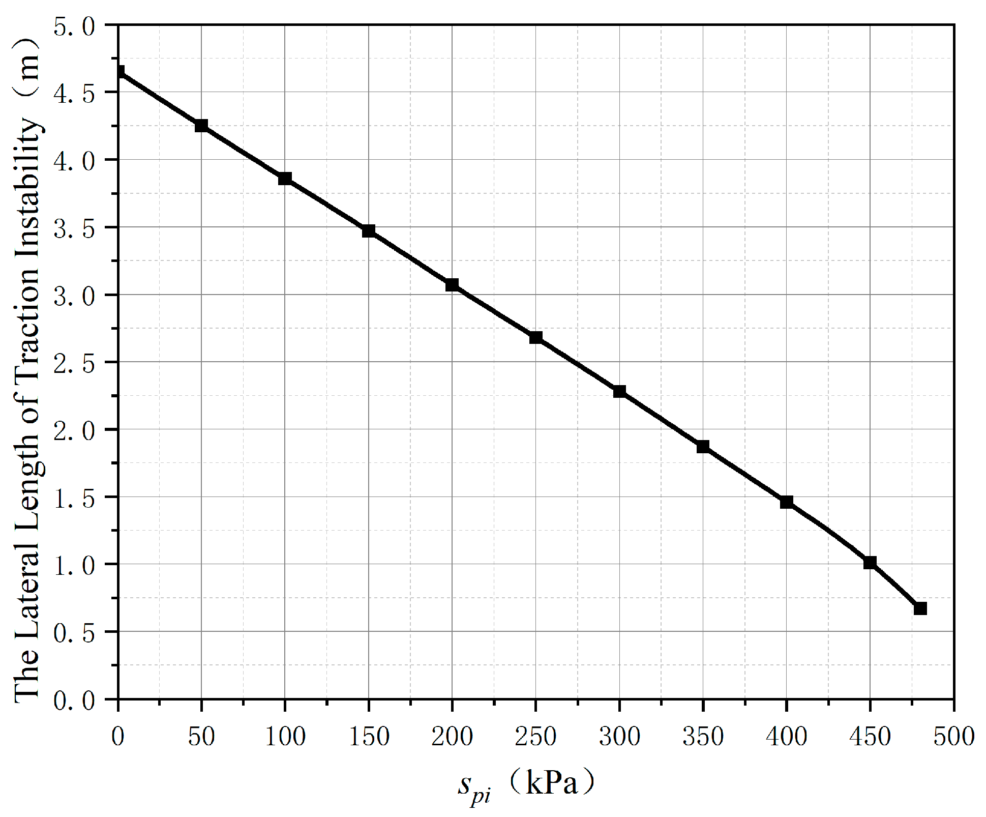
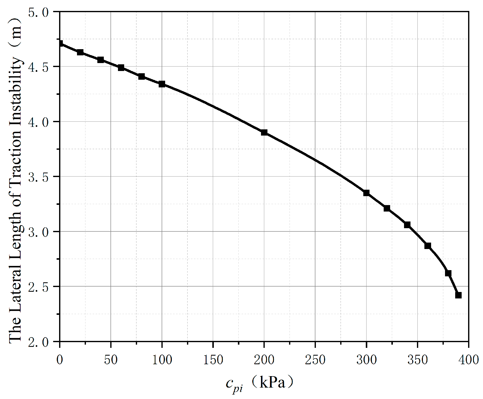
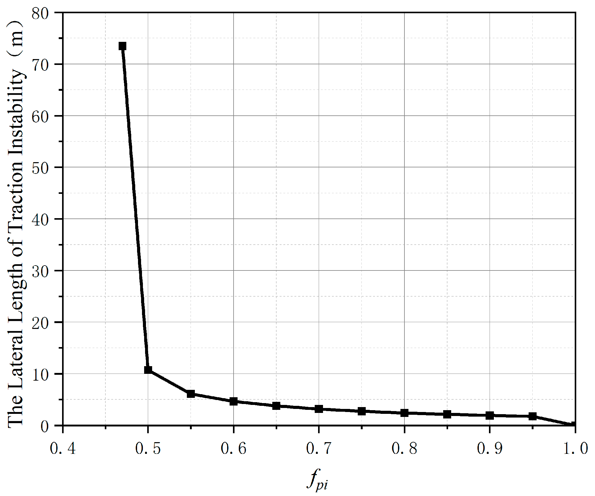
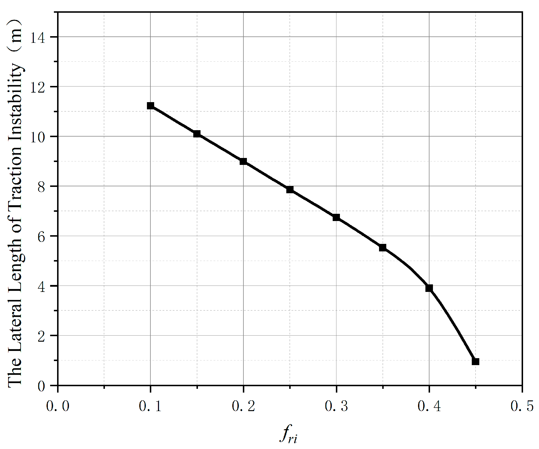
It can be seen from the above formula that the lateral length of traction instability when the slope is damaged is affected by many factors, including the dip angle of bedding, the friction coefficient, the bonding force, the tensile strength, and so on [57,58]. Analyzing the influence degree of these factors is helpful to judge the size of the landslide and roughly determine the range of slope instability in practical engineering. Based on this towed landslide, the influence of Spi, fpi, cpi, fri, and the dip angle of bedding on the lateral length of the slope traction instability is analyzed in detail.
Figure 14 shows the later length traction instability as a function of Spi (equivalent tensile strength of rock masses above the i-th layer that are not affected by excavation). It can be found that the curve is close to a straight line, which is a linear relationship. The influence of Spi on the lateral length of traction instability is relatively small, and it decreases by 0.8 m for every 100 kPa length increase. When Spi = 0 kPa, the lateral length of traction instability is the largest, which is 4.65 m. When Spi = 480 kPa, the slope is in a state of ultimate equilibrium.
Figure 15 shows the later length traction instability as a function of cpi (the cohesion of the bottom surface of the i-th layer that are not affected by excavation). It can be found that when cpi < 300 kpa, the curve is linear; when cpi > 300, the larger the cpi, the faster the lateral length of traction instability decreases, as shown in Figure 15. When cpi > 400 kPa, the slope tends to be stable. When cpi = 0 kPa, the lateral length of traction instability is the largest, which is 4.71 m. cpi is also not the main factor affecting the lateral length of slope traction instability.
Figure 16 shows the later length traction instability as a function of fpi (the friction coefficient of the bottom surface of the i-th layer that are not affected by excavation) [59,60]. The curve is almost at a right angle, as shown in Figure 16. When fpi > 0.5, the curve is relatively flat; when fpi < 0.5, the traction instability length increases sharply, and it reaches 73.5 m only when fpi = 0.47. This happens because the fpi is too small, resulting in the direct instability of the slope, and the upper rock mass will slide along with the lower rock mass of the slope without the phenomenon of segmented collapse. The lateral length of traction instability measured at this time is meaningless.
Figure 17 shows the later length traction instability as a function of fri (the friction coefficient of the bottom surface of the i-th layer most affected by excavation). The curve can also be divided into two parts, as shown in Figure 17. When fri < 0.35, the two are linear; when fri > 0.35, the larger the fri, the faster the lateral length of traction instability decreases. It can be seen that the two factors fpi and fri have a great influence on the lateral length of traction instability.
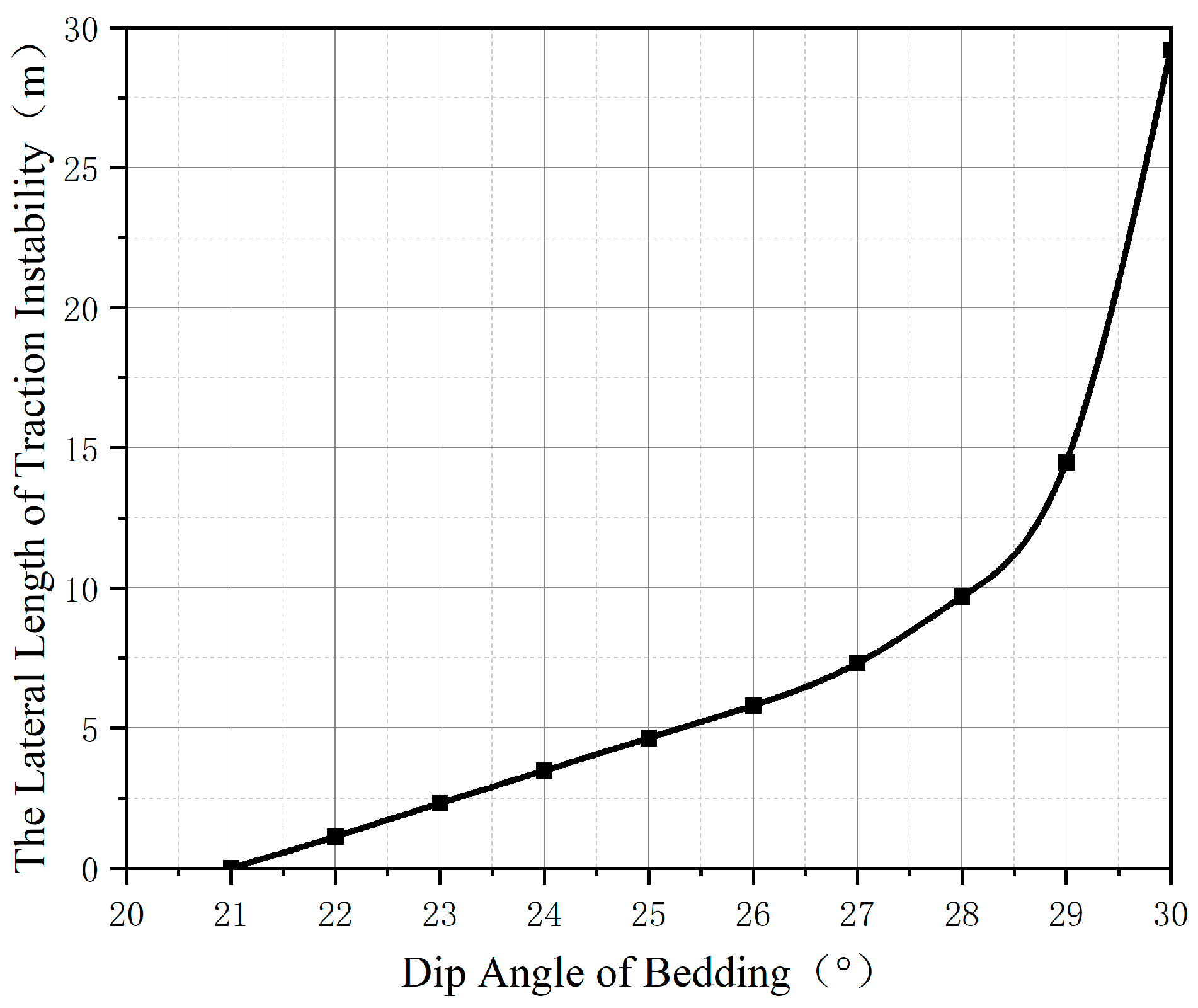
Figure 18 shows the later length traction instability as a function of the dip angle of bedding. It is found that the lateral length of the traction instability increases exponentially as shown in Figure 18. When the dip angle of bedding is less than or equal to 21°, the slope tends to be stable; when the dip angle of bedding is greater than 30°, the slope will be directly unstable, and the upper rock mass will slide together with the lower rock mass of the slope, without the phenomenon of segmented collapse. The dip angle of bedding is the most important factor affecting the lateral length of the traction instability.
The above results show that the dip angle of bedding is the most important factor affecting the lateral length of the slope traction instability, followed by fri and fpi, and the last is Spi and cpi. When roughly judging the range of slope instability in engineering practice, the main attention should be paid to the dip angle of bedding, the friction coefficient of the i-layer surface under the natural state, and the friction coefficient of the i-layer surface after the excavation are affected, and the vulnerable areas are first reinforced after comprehensive consideration.

4. Conclusions

(1)
The particle flow discrete element is used to simulate the complex geological conditions of the slope, and the total failure process of the retrogressive landslide is analyzed, and the mechanism of the slope failure is slip-pull crack according to previous research. The range of the first section of the slope is 4.54 m, that is, the first section of the slide area is located in the front 8.63% of the slope. This kind of slope will be pulled and split into multiple blocks when it slips, and the lower part of the slope will shift and cause the upper part to be unstable, and eventually slide along the sliding surface. The particle flow method has good applicability to simulate the failure movement process of the landslide.
(2)
When the retrogressive landslide is treated in engineering practice, the lateral length of the traction instability can be obtained according to the stability theory of the sliding pull-crack failure slope, and the accurate judgment of the traction failure range of the sliding body can be estimated.
(3)
The dip angle of bedding and the coefficient of friction are the main factors affecting the lateral length of the slope traction instability. In engineering practice, they should be mainly paid attention to when roughly judging slope instability.

Author Contributions

Conceptualization, X.Z., L.X. and H.L.; methodology, Y.T. and H.L.; formal analysis, X.Z. and Y.C.; investigation, H.H. and G.L.; resources, H.L. and H.H.; data curation, X.Z. and C.C.; writing—original draft preparation, X.Z. and L.X.; writing—review and editing, Y.T. and H.L. All authors have read and agreed to the published version of the manuscript.

Funding

This paper gets its funding from Project (NRMSSHR-2022-Z08) supported by Key Laboratory of Natural Resources Monitoring and Supervision in Southern Hilly Region, Ministry of Natural Resources; Hunan provincial key research and development Program (2022SK2082); Projects (42277175, 52104110) supported by National Natural Science Foundation of China; Science and Technology Progress and Innovation Plan of Hunan Provincial Department of Transportation (201003); Science and Technology Progress and Innovation Plan of Hunan Provincial Department of Transportation (202120). The authors wish to acknowledge these supports.

Institutional Review Board Statement

Not applicable.

Informed Consent Statement

Not applicable.

Data Availability Statement

The data used to support the findings of this study are available from the corresponding author upon request.

Conflicts of Interest

The authors declare no conflict of interest.

References

  1. Fan, H.; Lu, Y.; Hu, Y.; Fang, J.; Lv, C.; Xu, C.; Feng, X.; Liu, Y. A Landslide Susceptibility Evaluation of Highway Disasters Based on the Frequency Ratio Coupling Model. Sustainability 2022, 14, 7740. [Google Scholar] [CrossRef]
  2. Feng, T.; Chen, H.; Wang, K.; Nie, Y.; Zhang, X.; Mo, H. Assessment of underground soil loss via the tapering grikes on limestone hillslopes. Agric. Ecosyst. Environ. 2020, 297, 106935. [Google Scholar] [CrossRef]
  3. He, Y.; Zhong, G.; Wang, L.; Kuang, Z. Characteristics and occurrence of submarine canyon-associated landslides in the middle of the northern continental slope, South China Sea. Mar. Pet. Geol. 2014, 57, 546–560. [Google Scholar] [CrossRef]
  4. Lacroix, P.; Araujo, G.; Hollingsworth, J.; Taipe, E. Self-Entrainment Motion of a Slow-Moving Landslide Inferred From Landsat-8 Time Series. J. Geophys. Res. Earth Surf. 2019, 124, 1201–1216. [Google Scholar] [CrossRef]
  5. Zhang, X.; Wang, L.; Krabbenhoft, K.; Tinti, S. A case study and implication: Particle finite element modelling of the 2010 Saint-Jude sensitive clay landslide. Landslides 2020, 17, 1117–1127. [Google Scholar] [CrossRef] [Green Version]
  6. Yuan, Z.; Zhao, J.; Li, S.; Jiang, Z.; Huang, F. A Unified Solution for Surrounding Rock of Roadway Considering Seepage, Dilatancy, Strain-Softening and Intermediate Principal Stress. Sustainability 2022, 14, 8099. [Google Scholar] [CrossRef]
  7. Chen, C.; Peng, Z.; Gu, J.; Peng, Y.; Huang, X.; Wu, L. Exploring Environmentally Friendly Biopolymer Material Effect on Soil Tensile and Compressive Behavior. Int. J. Environ. Res. Public Health 2020, 17, 9032. [Google Scholar] [CrossRef]
  8. Zhu, C.; Long, S.; Zhang, J.; Wu, W.; Zhang, L. Time Series Multi-Sensors of Interferometry Synthetic Aperture Radar for Monitoring Ground Deformation. Front. Environ. Sci. 2022, 10, 929958. [Google Scholar] [CrossRef]
  9. Chigira, M.; Wang, W.-N.; Furuya, T.; Kamai, T. Geological causes and geomorphological precursors of the Tsaoling landslide triggered by the 1999 Chi-Chi earthquake, Taiwan. Eng. Geol. 2003, 68, 259–273. [Google Scholar] [CrossRef]
  10. Lian, B.; Peng, J.; Zhan, H.; Huang, Q.; Wang, X.; Hu, S. Formation mechanism analysis of irrigation-induced retrogressive loess landslides. Catena 2020, 195, 104441. [Google Scholar] [CrossRef]
  11. Richer, B.; Saeidi, A.; Boivin, M.; Rouleau, A. Overview of Retrogressive Landslide Risk Analysis in Sensitive Clay Slope. Geosciences 2020, 10, 279. [Google Scholar] [CrossRef]
  12. Del Gaudio, V.; Wasowski, J.; Pierri, P.; Mascia, U.; Calcagnile, G. Gravimetric Study of a Retrogressive Landslide in Southern Italy. Surv. Geophys. 2000, 21, 391–406. [Google Scholar] [CrossRef]
  13. Guo, C.; Zhang, Y.; Li, X.; Ren, S.; Yang, Z.; Wu, R.; Jin, J. Reactivation of giant Jiangdingya ancient landslide in Zhouqu County, Gansu Province, China. Landslides 2020, 17, 179–190. [Google Scholar] [CrossRef]
  14. Lollino, P.; Santaloia, F.; Amorosi, A.; Cotecchia, F. Delayed failure of quarry slopes in stiff clays: The case of the Lucera landslide. Géotechnique 2011, 61, 861–874. [Google Scholar] [CrossRef]
  15. Shan, Z.; Zhang, W.; Wang, D.; Wang, L. Numerical investigations of retrogressive failure in sensitive clays: Revisiting 1994 Sainte-Monique slide, Quebec. Landslides 2021, 18, 1327–1336. [Google Scholar] [CrossRef]
  16. Yang, T.; Rao, Y.; Wu, Y.; Wang, H.; Yu, Q.; Li, H.; Chen, H. Water softening-induced retrogressive landslides: Experiments and theoretical calculations of back scarp inclination. Geomorphology 2021, 389, 107800. [Google Scholar] [CrossRef]
  17. Zhang, W.; Wang, D. Stability analysis of cut slope with shear band propagation along a weak layer. Comput. Geotech. 2020, 125, 103676. [Google Scholar] [CrossRef]
  18. Lin, H.; Yu, Y.; Li, G.; Yang, H.; Peng, J. A Simplified Numerical Approach for the Prediction of Rainfall-Induced Retrogressive Landslides. Acta Geol. Sin.-Engl. Ed. 2016, 90, 1471–1480. [Google Scholar] [CrossRef]
  19. Marko, K.; Tiit, H.; Peeter, T.; Volli, K. Analysis of a retrogressive landslide in glaciolacustrine varved clay. Eng. Geol. 2010, 116, 109–116. [Google Scholar] [CrossRef]
  20. Lin, H.C.; Yu, Y.Z.; Li, G.X.; Peng, J.B. Developing Processes of Rainfall-induced Retrogressive Landslide by Model Experiments. Disaster Adv. 2012, 5, 861–865. [Google Scholar]
  21. Morandi, M.; Farabegoli, E.; Onorevoli, G. Root reinforcement and its implications in shallow landsliding susceptibility on a small alpine catchment. In Proceedings of the EGU General Assembly 2012, Conference Abstracts, Vienna, Austria, 22–27 April 2012; p. 4214. [Google Scholar]
  22. Li, Q.; Wang, Y.M.; Zhang, K.B.; Yu, H.; Tao, Z.Y. Field investigation and numerical study of a siltstone slope instability induced by excavation and rainfall. Landslides 2020, 17, 1485–1499. [Google Scholar] [CrossRef]
  23. Zheng, Y.; Chen, C.; Liu, T.; Xia, K.; Sun, C.; Chen, L. Analysis of a retrogressive landslide with double sliding surfaces: A case study. Environ. Earth Sci. 2020, 79, 21. [Google Scholar] [CrossRef]
  24. Li, J.; Chen, S.; Yu, F.; Jiang, L. Reinforcement Mechanism and Optimisation of Reinforcement Approach of a High and Steep Slope Using Prestressed Anchor Cables. Appl. Sci. 2020, 10, 266. [Google Scholar] [CrossRef] [Green Version]
  25. Liu, D.; Yang, X.; Wang, J. Study on Anti-Slide Pile Spacing in Slope Reinforcement Using Anti-Slide Pile with Geocell and Influencing Factors. In Proceedings of the 4th International Conference on Digital Manufacturing and Automation (ICDMA), Qingdao, China, 29–30 June 2013; IEEE: Piscataway Township, NJ, USA, 2013; pp. 1258–1260. [Google Scholar]
  26. Liu, Z.; Qiu, H.; Ma, S.; Yang, D.; Pei, Y.; Du, C.; Sun, H.; Hu, S.; Zhu, Y. Surface displacement and topographic change analysis of the Changhe landslide on September 14, 2019, China. Landslides 2021, 18, 1471–1483. [Google Scholar] [CrossRef]
  27. Zhou, T.; Luo, X.; Hou, Y.; Xiang, Y.; Peng, S. Quantifying the effects of road width on roadside vegetation and soil conditions in forests. Landsc. Ecol. 2020, 35, 69–81. [Google Scholar] [CrossRef] [Green Version]
  28. Li, M.; Lv, H.; Lu, Y.; Wang, D.; Shi, S.; Li, R. Instantaneous discharge characteristics and its methane ignition mechanism of coal mine rock damage. Environ. Sci. Pollut. Res. 2022, 29, 62495–62506. [Google Scholar] [CrossRef]
  29. Li, Y.; Zeng, X.; Lin, Z.; Su, J.; Gao, T.; Deng, R.; Liu, X. Experimental study on phosphate rock modified soil-bentonite as a cut-off wall material. Water Supply 2021, 22, 1676–1690. [Google Scholar] [CrossRef]
  30. Zhang, Y.; Ren, B.; Hursthouse, A.S.; Deng, R.; Hou, B. An Improved SWAT for Predicting Manganese Pollution Load at the Soil-Water Interface in a Manganese Mine Area. Pol. J. Environ. Stud. 2018, 27, 2357–2365. [Google Scholar] [CrossRef]
  31. Xie, Q.; Ren, B.; Hursthouse, A.; Shi, X. Effects of mining activities on the distribution, controlling factors, and sources of metals in soils from the Xikuangshan South Mine, Hunan Province. Integr. Environ. Assess. Manag. 2022, 18, 748–756. [Google Scholar] [CrossRef]
  32. Luo, X.; Ren, B.; Hursthouse, A.S.; Thacker, J.R.M.; Wang, Z. Soil from an Abandoned Manganese Mining Area (Hunan, China): Significance of Health Risk from Potentially Toxic Element Pollution and Its Spatial Context. Int. J. Environ. Res. Public Health 2020, 17, 6554. [Google Scholar] [CrossRef]
  33. Yu, S.; Chen, Y.; Zhao, J.; Fu, S.; Li, Z.; Xia, H.; Zhou, L. Temperature sensitivity of total soil respiration and its heterotrophic and autotrophic components in six vegetation types of subtropical China. Sci. Total Environ. 2017, 607, 160–167. [Google Scholar] [CrossRef] [PubMed]
  34. Yu, W.; Li, K.; Liu, Z.; An, B.; Wang, P.; Wu, H. Mechanical characteristics and deformation control of surrounding rock in weakly cemented siltstone. Environ. Earth Sci. 2021, 80, 1–15. [Google Scholar] [CrossRef]
  35. Zou, S.-H.; Li, K.-Q.; Han, Q.-Y.; Yu, C.W. Numerical simulation of the dynamic formation process of fog-haze and smog in transport tunnels of a hot mine. Indoor Built Environ. 2017, 26, 1062–1069. [Google Scholar] [CrossRef]
  36. Zhao, Y.; Luo, S.; Wang, Y.; Wang, W.; Zhang, L.; Wan, W. Numerical Analysis of Karst Water Inrush and a Criterion for Establishing the Width of Water-resistant Rock Pillars. Mine Water Environ. 2017, 36, 508–519. [Google Scholar] [CrossRef]
  37. Xie, W.; Ren, B.; Hursthouse, A.S.; Wang, Z.; Luo, X. Simulation of Manganese Transport in Groundwater Using Visual MODFLOW: A Case Study from Xiangtan Manganese Ore Area in Central China. Pol. J. Environ. Stud. 2020, 30, 1409–1420. [Google Scholar] [CrossRef] [PubMed]
  38. Potyondy, D.O. The bonded-particle model as a tool for rock mechanics research and application: Current trends and future directions. Geosyst. Eng. 2015, 18, 1–28. [Google Scholar] [CrossRef]
  39. Cundall, P.A. A computer model for simulating progressive, large-scale movement in blocky rock system. In Proceedings of the International Symposium on Rock Mechanics, Nancy, France, 4–6 October 1971. [Google Scholar]
  40. Cundall, P.A. Formulation of a three-dimensional distinct element model—Part I. A scheme to detect and represent contacts in a system composed of many polyhedral blocks. Int. J. Rock Mech. Mining Sci. Geomech. Abstr. 1988, 25, 107–116. [Google Scholar]
  41. Hart, R.; Cundall, P.A.; Lemos, J. Formulation of a three-dimensional distinct element model—Part II. Mechanical calculations for motion and interaction of a system composed of many polyhedral blocks. Int. J. Rock Mech. Mining Sci. Geomech. Abstr. 1988, 25, 117–125. [Google Scholar]
  42. Itasca Consulting Group, Inc. Universal Distinct Element Code, Version 5.0; Itasca Consulting Group, Inc.: Minneapolis, MN, USA, 2011. [Google Scholar]
  43. Liu, S.; Liu, H.; Liu, H.; Xia, Z.; Zhao, Y.; Zhai, J. Numerical simulation of mesomechanical properties of limestone containing dissolved hole and persistent joint. Theor. Appl. Fract. Mech. 2022, 122, 103572. [Google Scholar] [CrossRef]
  44. Ríos-Bayona, F.; Johansson, F.; Mas-Ivars, D.; Sánchez-Juncal, A.; Bolin, A. Using PFC2D to simulate the shear behaviour of joints in hard crystalline rock. Bull. Eng. Geol. Environ. 2022, 81, 1–19. [Google Scholar] [CrossRef]
  45. Li, B.; Gong, W.; Tang, H.; Zou, Z.; Bowa, V.M.; Juang, C.H. Probabilistic analysis of a discrete element modelling of the runout behavior of the Jiweishan landslide. Int. J. Numer. Anal. Methods Geomech. 2021, 45, 1120–1138. [Google Scholar] [CrossRef]
  46. Yin, Z.; Li, R.; Lin, H.; Chen, Y.; Wang, Y.; Zhao, Y. Analysis of Influencing Factors of Cementitious Material Properties of Lead–Zinc Tailings Based on Orthogonal Tests. Materials 2023, 16, 361. [Google Scholar] [CrossRef]
  47. Zhang, N.-C.; Zhang, N.; Esterle, J.; Kan, J.-G.; Zhao, Y.-M.; Xue, F. Optimization of gateroad layout under a remnant chain pillar in longwall undermining based on pressure bulb theory. Int. J. Mining Reclam. Environ. 2016, 30, 128–144. [Google Scholar] [CrossRef]
  48. Liu, S.; Nie, Y.; Hu, W.; Ashiru, M.; Li, Z.; Zuo, J. The Influence of Mixing Degree between Coarse and Fine Particles on the Strength of Offshore and Coast Foundations. Sustainability 2022, 14, 9177. [Google Scholar] [CrossRef]
  49. Wu, H.; Jia, Q.; Wang, W.; Zhang, N.; Zhao, Y. Experimental Test on Nonuniform Deformation in the Tilted Strata of a Deep Coal Mine. Sustainability 2021, 13, 13280. [Google Scholar] [CrossRef]
  50. Lu, Y.; Liu, Y.; Shi, S.; Wang, G.G.; Li, H.; Wang, T. Micro-particles stabilized aqueous foam for coal spontaneous combustion control and its flow characteristics. Process Saf. Environ. Prot. 2020, 139, 262–272. [Google Scholar] [CrossRef]
  51. Zhao, Y.; Zhang, C.; Wang, Y.; Lin, H. Shear-related roughness classification and strength model of natural rock joint based on fuzzy comprehensive evaluation. Int. J. Rock Mech. Min. Sci. 2021, 137, 104550. [Google Scholar] [CrossRef]
  52. Chen, W.; Wan, W.; Zhao, Y.; Peng, W. Experimental Study of the Crack Predominance of Rock-Like Material Containing Parallel Double Fissures under Uniaxial Compression. Sustainability 2020, 12, 5188. [Google Scholar] [CrossRef]
  53. Zhao, Y.; Tang, J.; Chen, Y.; Zhang, L.; Wang, W.; Wan, W.; Liao, J. Hydromechanical coupling tests for mechanical and permeability characteristics of fractured limestone in complete stress–strain process. Environ. Earth Sci. 2017, 76, 1–18. [Google Scholar] [CrossRef]
  54. Zhao, Y.; Liu, Q.; Zhang, C.; Liao, J.; Lin, H.; Wang, Y. Coupled seepage-damage effect in fractured rock masses: Model development and a case study. Int. J. Rock Mech. Min. Sci. 2021, 144, 104822. [Google Scholar] [CrossRef]
  55. Liu, J.; Zhao, Y.; Tan, T.; Zhang, L.; Zhu, S.; Xu, F. Evolution and modeling of mine water inflow and hazard characteristics in southern coalfields of China: A case of Meitanba mine. Int. J. Min. Sci. Technol. 2022, 32, 513–524. [Google Scholar] [CrossRef]
  56. Peng, Y.; Liu, G.; Wu, L.; Zuo, Q.; Liu, Y.; Zhang, C. Comparative study on tunnel blast-induced vibration for the underground cavern group. Environ. Earth Sci. 2021, 80, 1–13. [Google Scholar] [CrossRef]
  57. Tang, H.; Yong, R.; Ez Eldin, M.A.M. Stability analysis of stratified rock slopes with spatially variable strength parameters: The case of Qianjiangping landslide. Bull. Eng. Geol. Environ. 2017, 76, 839–853. [Google Scholar] [CrossRef]
  58. Xia, G.Q.; Liu, C.; Xu, C.; Le, T.C.; Foong, L. Dynamic Analysis of the High-Speed and Long-Runout Landslide Movement Process Based on the Discrete Element Method: A Case Study of the Shuicheng Landslide in Guizhou, China. Adv. Civ. Eng. 2021, 2021, 1–16. [Google Scholar] [CrossRef]
  59. Wang, F.; Sassa, K. Landslide simulation by a geotechnical model combined with a model for apparent friction change. Phys. Chem. Earth, Parts A/B/C 2010, 35, 149–161. [Google Scholar] [CrossRef]
  60. Tang, C.-L.; Hu, J.-C.; Lin, M.-L.; Angelier, J.; Lu, C.-Y.; Chan, Y.-C.; Chu, H.-T. The Tsaoling landslide triggered by the Chi-Chi earthquake, Taiwan: Insights from a discrete element simulation. Eng. Geol. 2009, 106, 1–19. [Google Scholar] [CrossRef]
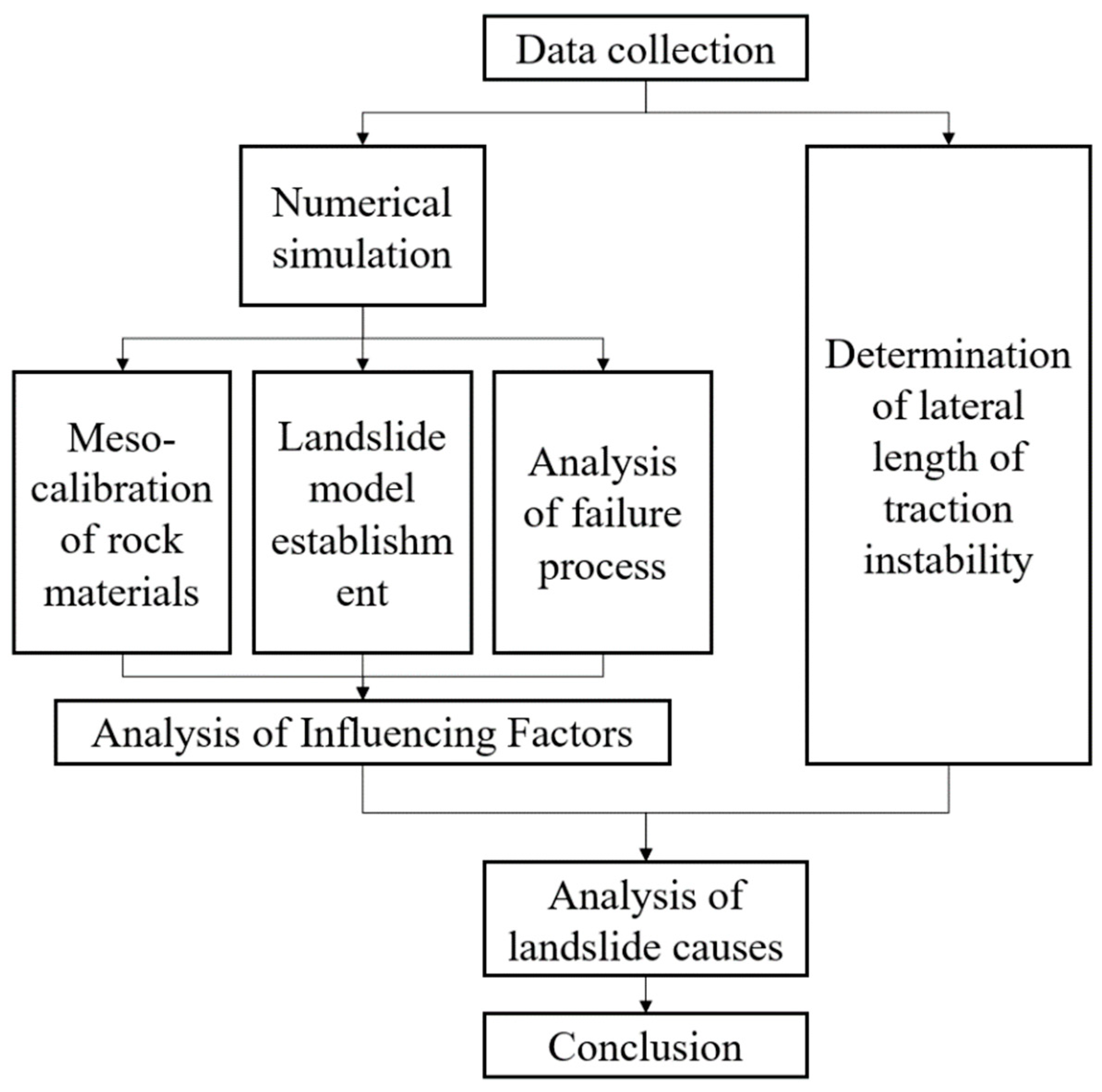
Figure 1. Technical flow chart.
Applsci 13 00799 g001
Figure 2. Geological map of the landslide section.
Applsci 13 00799 g002
Figure 3. Landslide.
Applsci 13 00799 g003
Figure 4. The stratigraphic lithology division.
Applsci 13 00799 g004
Figure 5. CAD schematic diagram of slope section.
Applsci 13 00799 g005
Figure 6. Schematic diagram of the Parallel-Bond Model.
Applsci 13 00799 g006
Figure 7. Slope model.
Applsci 13 00799 g007
Figure 8. Displacement diagram in the early stage of slope collapse.
Applsci 13 00799 g008
Figure 9. Displacement diagram in the middle of the collapse.
Applsci 13 00799 g009
Figure 10. Displacement diagram in the later stage of collapse.
Applsci 13 00799 g010
Figure 11. Displacement diagram of complete failure of the slope.
Applsci 13 00799 g011
Figure 12. Slope calculation model.
Applsci 13 00799 g012
Figure 13. PFC2D rock mass displacement diagram.
Applsci 13 00799 g013
Figure 14. Influence of Spi on the lateral length of traction instability.
Applsci 13 00799 g014
Figure 15. Influence of cpi on the lateral length of traction instability.
Applsci 13 00799 g015
Figure 16. Influence of fpi on the lateral length of traction instability.
Applsci 13 00799 g016
Figure 17. Influence of fri on the lateral length of traction instability.
Applsci 13 00799 g017
Figure 18. Influence of the Dip Angle of Bedding on the lateral length of traction instability.
Applsci 13 00799 g018
Table 1. Strong weathered calcium argillaceous sandstone.
Simulation ParametersNumerical Value
Normal stiffness2.28
Linear method deform friction angle (°)21
Linear method deform tensile strength (MP)3.0
Linear method deform adhesion (MP)3.0
Particle density (kg/m3)2600
Table 2. Medium weathered calcareous mudstone.
Simulation ParametersNumerical Value
Normal stiffness2.0
Linear method deform friction angle (°)21
Linear method deform tensile strength (MP)2.48
Linear method deform adhesion (MP)2.4
Particle density (kg/m3)2600
Table 3. Medium weathered calcareous sandstone.
Simulation ParametersNumerical Value
Normal stiffness2.0
Linear method deform friction angle (°)21
Linear method deform tensile strength (MP)35
Linear method deform adhesion (MP)35
Particle density (kg/m3)2600
Table 4. Calcareous sandstone.
Simulation ParametersNumerical Value
Normal stiffness1.52
Linear method deform friction angle (°)21
Linear method deform tensile strength (MP)54
Linear method deform adhesion (MP)54
Particle density (kg/m3)2600
Disclaimer/Publisher’s Note: The statements, opinions and data contained in all publications are solely those of the individual author(s) and contributor(s) and not of MDPI and/or the editor(s). MDPI and/or the editor(s) disclaim responsibility for any injury to people or property resulting from any ideas, methods, instructions or products referred to in the content.