Abstract
A conventional dynamic vibration absorber based on resonance effect can hardly satisfy the requirement for low-frequency and broadband vibration control in actual engineering. Combined with passive and nonlinear vibration absorption strategy, this study employed nonlinear characteristics of the magnetic force, bistable structure to establish the dynamic model of the main system with a bistable vibration absorber. The nonlinear motion states of the structure under different excitation conditions were analyzed to explore the inherent relation between the chaotic and large amplitude motion and the vibration absorber’s operating performance. The effect laws of the structural parameters on the dynamic characteristics of the nonlinear vibration absorber and the main system were developed to obtain the optimal parameter settings in the case of resonance and off-resonance of the main system. These results provide an insightful theoretical foundation for the optimal design of the nonlinear vibration absorber.
1. Introduction
A traditional passive vibration attenuation system mainly utilizes certain materials or damping elements, such as a rubber shock absorber, metal spring or air spring, for counteracting the vibration force; however, the natural frequency can hardly be lowered, on account of the contradiction between low rigidity and the static bearing capacity [1,2,3]. Recently, for low-frequency vibration control, scholars mainly adopt an air spring, variable-stiffness spring or multi-level vibration reduction system [4,5,6]. Despite effective reduction of the natural frequency of the vibration reduction system, these vibration reduction measures can hardly be extensively applied in actual projects because of the complex structure, the high cost, the great energy consumption and the addition of a control system [7].
In order to address the issue of a traditional vibration absorber not being applicable to a low-frequency environment, some scholars have introduced nonlinear elastic elements into vibration absorbing systems and designed a kind of nonlinear absorber. By setting reasonable parameters, the dynamic characteristics of the nonlinear vibration absorber are subjected to static load, so it can keep low stiffness while maintaining large bearing capacity, thereby achieving vibration absorption at low or ultra-low frequencies. Virgin et al. designed a nonlinear vibration absorber, which can achieve the preset dynamic stiffness, under a given static loading condition, while the constraint of deformation is based on the geometric nonlinearity of large-deformation elastic elements [8]. Guest focused on thin cylindrical shell structures which can show interesting bistable behavior [9]. Zhao et al. investigated the coupled modeling method and free vibration characteristics of a graphene nanoplatelet (GPL)-reinforced blade–disk rotor system in which the blade has a pre-twist angle and a setting angle [10,11]. Moreover, they presented an investigation on the coupled modeling and vibration behaviors of a spinning assembled cylindrical shell–plate structure. The method of hypothesis modes was adopted to obtain the free vibration results of the assembled cylindrical shell–plate structure [12]. Using Timoshenko’s and Ashwell’s approaches, Nicassio developed an interpretation of the bistable shapes, in terms of principal and anticlastic curvatures [13]. Kremer and Liu employed a nonlinear absorber for energy collection and examined the vibration-absorbing and energy-collecting performance of the absorber, under instantaneous response conditions via computer simulation, and they experimentally validated the simulation results [14,15]. By improving the single-pendulum nonlinear vibration damping system, scholars successively put forward an inverted-pendulum, transverse-pendulum, X-pendulum and conical-pendulum ultra-low-frequency horizontal vibration absorption system that can achieve a resonance period, from several seconds to dozens of seconds [16,17,18,19,20,21]. Further, Shapiro et al. used a symmetrical-torsion-bar spring, multi-level vibration-isolation absorber, a yield cylinder (Euler spring) and a negative-rigidness spring to realize passive absorption of low-frequency vibration, in a vertical direction [22,23,24]. Zhao et al. investigated the free vibration of a rotating functionally graded (FG), pre-twisted blade-shaft assembly reinforced with graphene nanoplatelets (GPLs) based on the coupled model proposed in this paper [25]. Moreover, they developed a super-parametric shell element to establish the rotating cylindrical shell model by employing the finite element method. Considering parameter uncertainties, the dynamic response of the rotating cylindrical shell is carried out [26]. Yan et al. presented a method to easily and rapidly design bistable buckled beams subjected to a transverse point force [27].
In this study, based on passive and nonlinear vibration absorption strategy, a magnetic bistable vibration-absorbing structure was established by introducing a nonlinear magnetic force and changing the dynamic characteristics of the magnetic suspension vibration absorber. The dynamic model for the main system with a bistable vibration-absorbing structure was constructed. Through numerical simulation, the influencing rules of large amplitude motion and structural parameters (namely, the tuning frequency ratio f, the mass ratio μ, the nonlinear intensity β and the damping coefficient of the vibration absorber γ1) were studied, and the parameter setting for improving the vibration absorber’s operating efficiency was concluded when the main system was under resonance and off-resonance states.
2. System Vibration Model
2.1. Dynamic Model
Figure 1 displays two steady-state forms of the bistable unit model. The model consists of two mutually exclusive permanent magnets and a bistable cantilever beam vibrator. The cantilever beam is made up of Aluminum (Al) materials. A magnet is fixed at the end of the cantilever, which is opposite to the other fixed magnet. The repulsive force between two magnets forms a bistable structure. Because of the repulsion between the two magnets, when the whole system is at rest, three equilibrium positions are formed. By following the horizontal straight line that passes through the center of the fixed magnet on the right as the datum, the three equilibrium positions lie along this horizontal straight line, above and below the straight line, respectively. Among these three positions, the equilibrium position on the horizontal straight line is the unstable equilibrium position. This is because some tiny turbulence can cause the shift of the system due to large repulsive force. Excluding the unstable equilibrium position, the other two positions are referred to as stable equilibrium positions, which constitute the bistable structure of the cantilever beam. The frequency resonance bandwidth of the bistable vibration system exceeds that of the linear vibration system. This is due to the fact that only when the natural frequency of the system, ωn, is equal to or close to the external excitation frequency, ω, can the linear system produce the forced vibration. Bistable vibration can not only generate forced vibration at a frequency of ωn but also produce sub-resonance at a frequency of ω/n or ultra-harmonic vibration at a frequency of nω and even aperiodic vibration. The broadband frequency of the bistable resonance can effectively overcome the problem of too narrow resonant frequency bandwidth in the traditional linear vibration system.
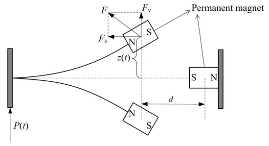
Figure 1.
The bistable structural unit.
Figure 2 displays the mechanical model of the main system with a bistable vibration absorber, in which m1 and m2 are the equivalent masses of the permanent magnets and the main system, respectively; c1 and c2 are the damping coefficients of the absorber and the main system, respectively; k2 is the stiffness of the main spring; Y and Z are the absolute displacements of the main system and the absorber, respectively; X = Y − Z denotes the relative displacement between the absorber and the main system; dU/dX = −k1X + k3X3 denotes the bistable spring restoring force of the absorber (U is the elastic potential energy of the nonlinear spring, k1 is the linear stiffness coefficient, k3 is the nonlinear stiffness coefficient of the bistable absorber); P denotes the excitation force, applied to the main system.
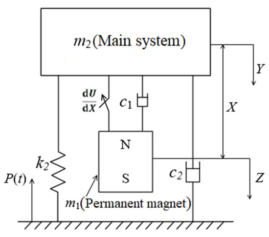
Figure 2.
Mechanical model of the main system.
The governing equation of the system can be written as:
By conducting nondimensionalization on Equations (1) and (2), the following expression can be obtained:
where ; ; ; ; ; ; t denotes the dimensionless time (); p denotes the excitation amplitude (); ω denotes the excitation frequency (); μ denotes the mass ratio (); f denotes the tuning frequency ratio (); β denotes the nonlinear intensity (); γ1 denotes the damping ratio of the absorber (); and γ2 denotes the damping ratio of the main system ().
2.2. Experimental Validation
In order to validate the dynamic model established in this research, the testbench was installed, and the corresponding experiment was conducted. The testbench consisted of the base, the upper cover which acted as the main system and the bolts between them. The pretighting torque could be adjusted by a torque wrench, shown in Figure 3. The vibration absorber was fixed on the top of the upper cover to suppress the vibration. The vibration absorber contained the beam, which acted as the spring component, and the permanent magnets, depicted in Figure 3. Two permanent magnets were used in the vibration absorber. One was pasted at the end of beam, the other was attached on the steel wall. The beam is made of aluminum alloy to reduce the effect of the beam’s mass. An accelerometer was attached at the end of the beam, and the system was stimulated by a hammer with a force sensor. According to the collected data, the direct frequency response function (FRF) at the end of the beam was determined with the Metalmax system. The experimental result is shown in Figure 3. From the experimental FRF, the first nature frequency is 629 Hz.
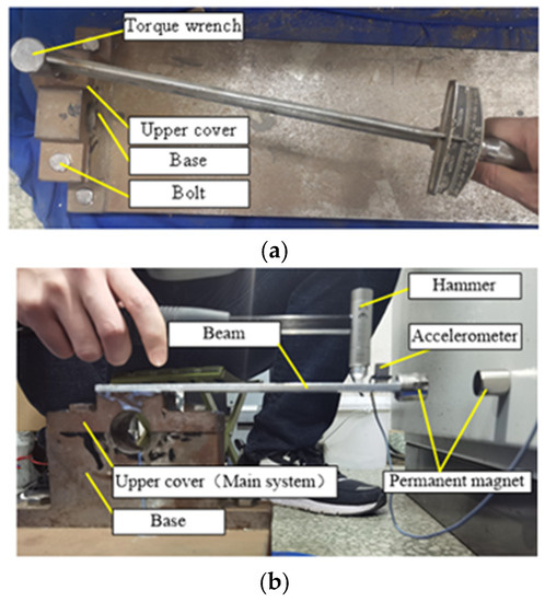
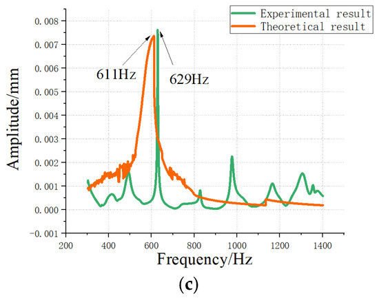
Figure 3.
Experimental process. (a) Pretighting torque adjustment; (b) Dynamic test of experimental setup; (c) Experimental result.
The dynamic parameters of the interface between the upper cover and the base can be determined with the Yoshimura integral method. According to the dynamic model established in this research, the theoretical result of the first nature frequency is calculated as 611 Hz. The error between the experimental result and the theoretical one is 3%. The experimental result is slightly greater than the theoretical. That is because the nonlinearity of the magnetic force is ignored in the nature frequency calculation. The nature frequency calculation must be a linear calculation process with the nonlinear factor ignored. The actual stiffness factor is greater than that in the calculation, which causes the actual nature frequency to be greater than that in the calculation. However, the error between them is relatively small, and the dynamic model in this research is validated.
3. Analysis of Dynamic Parameters
In order to investigate the dynamic response of the bistable vibration absorber and the main system under harmonic excitation, the dimensionless Equations (3) and (4) were solved, using Simulink simulation to sweep frequency and amplitude, in terms of fundamental excitation frequency and the amplitude of the system. The simulation parameters were β = 1.0, μ = 0.3, f = 1.0, γ1 = 0.05, γ2 = 0.05, and the initial value of the system [x x′ y y′] was set to [0 0 0 0].
3.1. Effects of the Excitation Frequency on the Response Characteristics of the Vibration Absorber and the Main System
Figure 4 shows the bifurcation phenomenon of the vibration absorber and the main system at an excitation amplitude of p = 0.01, p = 0.15 and p = 0.5. As shown in Figure 4a (excitation amplitude p = 0.01), the absorber never overcame the potential barrier in the whole excitation frequency range, while there was only slight motion around the equilibrium point x = −1. In Figure 4b (excitation amplitude p = 0.15), when excitation frequency ω = 0–0.5, the absorber performed slight motion at and around the equilibrium point x = −1; when ω = 0.7–1.7, the absorber could overcome the potential barrier and showed large amplitude motion between two equilibrium points, while the main system also performed large amplitude motion; when ω > 1.7, the system began to show slight motion. Compared with Figure 4b (p = 0.15) and Figure 4c (p = 0.5), the large amplitude motion frequency of the absorber and the main system decreased, and the frequency band of the large amplitude motion became wider as the excitation amplitude increased. However, as the excitation frequency further increased, the absorber changed its state from large amplitude motion to slight motion around an equilibrium point.
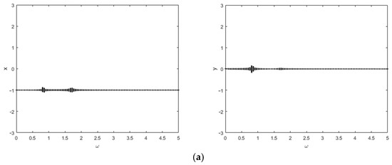
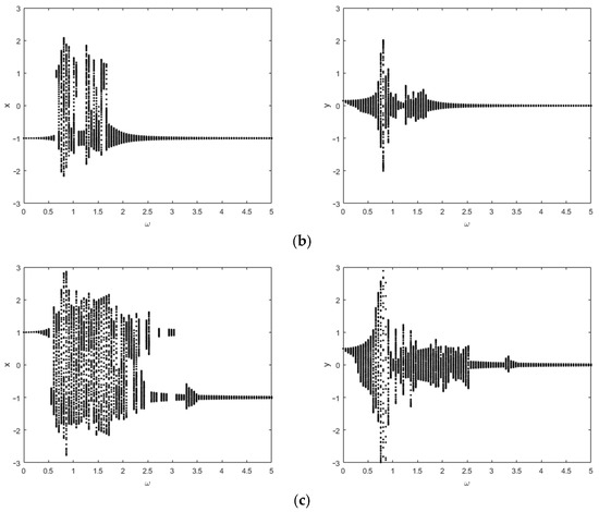
Figure 4.
Bifurcation of the vibration absorber (on the left side) and the main system (on the right side) along excitation frequency at different excitation amplitudes. (a) Excitation amplitude p = 0.01; (b) Excitation amplitude p = 0.15; (c) Excitation amplitude p = 0.5.
To visually display the change in the system motion characteristics, the corresponding system phase diagrams at excitation frequency ω = 2 and excitation amplitude p = 0.1 and 0.5 are plotted in Figure 5. It can be observed that, at a constant excitation frequency, the vibration absorber and main system changed from slight periodic motion to large amplitude chaotic motion with excitation amplitude increasing.
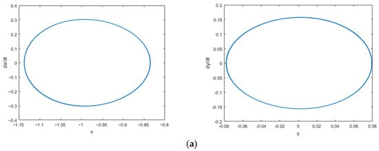
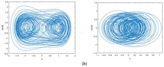
Figure 5.
Phase diagrams of the vibration absorber (on the left side) and the main system (on the right side) at different excitation amplitudes. (a) ω = 2, p = 0.15; (b) ω = 2, p = 0.5.
3.2. Effects of the Excitation Amplitude on the Response Characteristics of the Vibration Absorber and the Main System
Figure 6 shows the bifurcations of the vibration absorber and the main system with the excitation amplitude when the excitation frequency is ω = 0.1, ω = 0.5, ω = 1, ω = 2 and ω = 3.5. As shown in Figure 6a (ω = 0.1), even at a quite low excitation frequency, the absorber can cross the potential barrier from an equilibrium point to another equilibrium point, while the main system executes slight motion around the equilibrium point. In contrast, as shown in Figure 6b–d, as the excitation frequency increased, the absorber performed slight motion around the equilibrium point, and the main system executed a slight motion around the zero-equilibrium point. As the excitation amplitude increased, both the absorber and the main system performed large amplitude chaotic or period motions. Moreover, as the excitation frequency increased, the required excitation amplitude for the absorber and the main system to perform large amplitude motions first decreased and then increased. As shown in Figure 6e (ω = 3.5), as the excitation frequency increased to a certain value, the absorber failed in overcoming the potential barrier and executed only slight motion around the equilibrium point x = −1, while the main system also performed slight motion at any excitation amplitude.
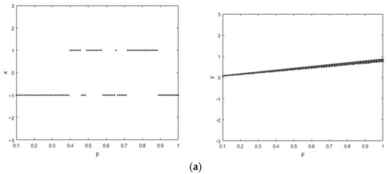
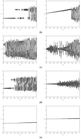
Figure 6.
Bifurcation of the vibration absorber (on the left side) and the main system (on the right side) along excitation amplitude at different excitation frequencies. (a) Excitation frequency ω = 0.1; (b) Excitation frequency ω = 0.5; (c) Excitation frequency ω = 1; (d) Excitation frequency ω = 2; (e) Excitation frequency ω = 3.5.
When the excitation amplitude remained constant (p = 0.7) and the excitation frequency changed (ω = 0.1, ω = 2 and ω = 3), phase diagrams of the system are shown in Figure 7. The vibration absorber and main system first performed slight periodic motion, then executed large amplitude chaotic motion and finally changed to slight period motion.
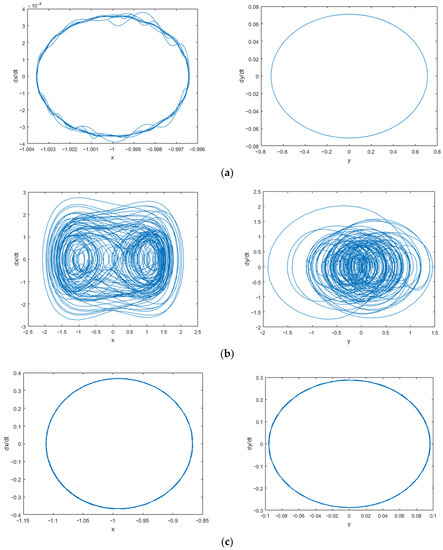
Figure 7.
Phase diagrams of the absorber (on the left side) and the main system (on the right side) at different excitation frequencies. (a) p = 0.7, ω = 0.1; (b) p = 0.7, ω = 2; (c) p = 0.7, ω = 3.
4. Effects of the Structural Parameters
To achieve a favorable vibration damping effect, various optimal parameters should be determined to ensure that the vibration absorber could operate under the optimal condition. Regarding the design of an absorber, the resonance, when the excitation frequency is close to the natural frequency of the main system, is most dangerous; at that time, the damping should first be ensured. Therefore, in the case of resonance of the main system, the vibration absorber should maximize the damping effect to minimize the amplitude of the main system; in the case of off-resonance of the main system, the vibration absorber should not only maintain a low amplitude of the main system but also maximize its own amplitude. Based on the above optimization condition, the vibration absorber’s optimal parameters are analyzed in resonance and off-resonance.
4.1. Tuning Frequency Ratio f
The present simulation parameters are set as follows: β = 1.0, μ = 0.3, γ1 = 0.025 and γ2 = 0.025. Figure 8a shows the system response amplitude in relation to the tuning frequency ratio f, in the case of resonance of the main system at ω = 1.0. Overall, the main system and the vibration absorber first decreased and then remained constant as f changed. According to the optimization condition of resonance, the amplitude of the main system should be minimized, so the optimal tuning frequency ratio f was set at 1.4–2.0. Taking the condition f = 1.7 as an example, Figure 8b shows the phase diagram of the main system, which shows that the main system executed slight periodic motion while the vibration absorber was operating at a high efficiency.
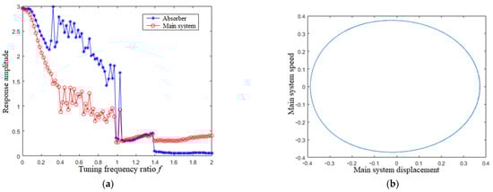
Figure 8.
Response amplitude of two vibrators and phase diagram of the main system in the case of resonance ω = 1.0. (a) Response amplitude; (b) Phase diagram (f = 1.7).
In the case of off-resonance of the main system at an off-resonance excitation frequency ω = 0.6, the system response amplitude as f changed is shown in Figure 9a. When f = 0.2–0.6, the main system performed lower amplitude motion while the amplitude of the vibration absorber was higher; when f > 0.8, the absorber performed slight motion. According to the optimization condition of off-resonance, the vibration absorber should not only maintain a low amplitude of the main system but also maximize its own amplitude, so the optimal tuning frequency ratio f was determined at 0.2–0.6. Taking f = 0.5 as an example, the phase diagram of the vibration absorber and the main system was plotted in Figure 9b. The absorber performed a large chaotic motion, while the main system moved in a small amplitude.
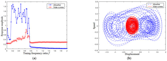
Figure 9.
Response amplitude and phase diagram of two vibrators in the case of off-resonance ω = 0.6. (a) Response amplitude; (b) Phase diagram (f = 0.5).
Figure 10a shows the system response amplitude in relation to the increasing f at an off-resonance excitation frequency ω = 1.6. Apparently, the optimal value of f was determined to be 0.8–1.0. Figure 10b displays the phase diagrams of two vibrators at f = 0.9. It can be observed that the vibration absorber could overcome the potential barrier and performed large amplitude chaotic motion, while the main system executed a slight motion.
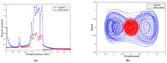
Figure 10.
Response amplitude and phase diagram of two vibrators in the case of off-resonance ω = 1.6. (a) Response amplitude; (b) Phase diagram (f = 0.9).
4.2. Mass Ratio μ
In this section, the effects of the mass ratio μ on the dynamic responses of the vibration absorber and the main system are investigated. According to the analysis results, presented in Section 4.1, the simulation parameter f can be set as follows: when ω = 1.0, f was set at 1.5; when ω = 0.6, f was set at 0.25; when ω = 1.6, f was set at 1.0, during which β = 1.0, γ1 = 0.025 and γ2 = 0.025.
Figure 11a shows the response amplitude of the vibration absorber and the main system in relation to the mass ratio, μ, in the case of main system resonance ω = 1.0. It can be observed that when μ > 0.2, the main system amplitude decreased to the minimum and converged to a constant value. Thus, the range of optimal mass ratio μ was determined as 0.2–0.5. Figure 11b shows the phase diagram of the main system at μ = 0.4, with which it is evident that the main system performed periodic motion with slight amplitude.
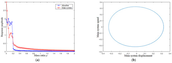
Figure 11.
Response amplitude of two vibrators and phase diagram of main system in the case of resonance ω = 1.0. (a) Response amplitude; (b) Phase diagram (μ = 0.4).
Figure 12 shows the response amplitude of the vibration absorber and the main system as μ increases and the related phase diagram at an off-resonance excitation frequency ω = 0.6. As shown in Figure 12a, the absorber was always performing large amplitude motion, and the main system executed slight motion. The amplitude of the absorber decreased gradually and finally stabilized, while the amplitude of the main system increased steadily and finally converged to a constant value. Therefore, the optimal mass ratio μ’s range was determined as 0.01–0.5. Meanwhile, the phase diagrams of the absorber and the main system at μ = 0.2 (within a range of 0.01–0.50) were plotted, as shown in Figure 12b. It can be observed that the absorber executed large amplitude chaotic motion and the main system performed slight motion.
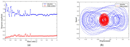
Figure 12.
Response amplitude and phase diagram of two vibrators in the case of off-resonance ω = 0.6. (a) Response amplitude; (b) Phase diagram (μ = 0.2).
Figure 13 shows the response amplitude of the vibration absorber and the main system as μ increases and the related phase diagram at an off-resonance excitation frequency ω = 1.6. As shown in Figure 13a, when the mass ratio μ varied within the range of 0.1–0.6, the absorber executed large amplitude motion, and the main system performed slight motion. As the mass ratio μ > 0.8, the absorber and the main system performed slight motions. Apparently, according to the optimization condition of off-resonance, the range of optimal mass ratio μ was determined as 0.1–0.6. Figure 13b is the phase diagram of the absorber and the main system at μ = 0.4. The main system performed slight motion, and the absorber showed bifurcation and overcame the potential barrier many times, executing large amplitude chaotic motion.
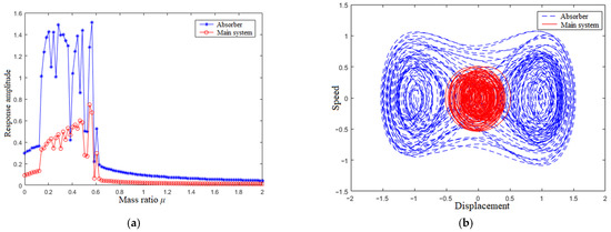
Figure 13.
Response amplitude and phase diagram of two vibrators in the case of off-resonance ω = 1.6. (a) Response amplitude; (b) Phase diagram (μ = 0.4).
4.3. Nonlinear Intensity β
Based on the simulation results, as presented in Section 4.1 and Section 4.2, some reasonable parameters are listed below when the amplitude of the vibration absorber was lower than that of the main system. When ω = 1.0, the other parameters can be set as follows: μ = 0.35, f = 1.5, γ1 = 0.025 and γ2 = 0.025; when ω = 0.6, the other parameters can be fixed as follows: μ = 0.3, f = 0.25, γ1 = 0.025, γ2 = 0.025; when ω = 1.6, the other parameters can be fixed as follows: μ = 0.3, f = 1.0, γ1 = 0.025, γ2 = 0.025.
As shown in Figure 14a, in the case of system resonance ω = 1.0, when nonlinear intensity β < 1, the amplitude of the main system and the vibration absorber varied slightly; when β > 1, the two vibrators moved unstably and exhibited high sensitivity. Therefore, the optimal range of β, corresponding to the minimum amplitude of the main system, was determined as 0.1–1. Figure 14b shows the response characteristics of the main system when β = 0.7; the main system performed slight periodic motion.
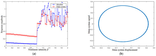
Figure 14.
Response amplitude of two vibrators and phase diagram of main system in the case of resonance ω = 1.0. (a) Response amplitude; (b) Phase diagram (β = 0.7).
Figure 15a shows the variation of the response amplitude of two vibrators at off-resonance excitation frequency ω = 0.6. As β increased, the main system performed slight and stable motion, while the vibration absorber executed large amplitude motion with decreasing amplitude. According to the optimization condition of off-resonance, the optimal range of β was then determined as 0.10–0.40. Figure 15b shows the phase diagrams of the vibration absorber and the main system, at β = 0.3. The absorber performed large amplitude periodic motion, while the main system performed slight periodic motion with clearly decreasing amplitude.
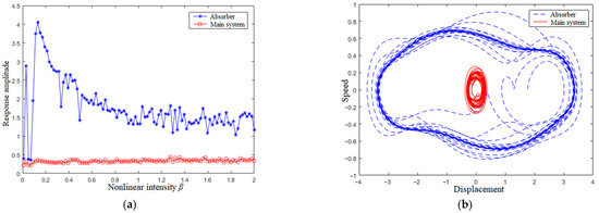
Figure 15.
Response amplitude and phase diagram of two vibrators in the case of off-resonance ω = 0.6. (a) Response amplitude; (b) Phase diagram (β = 0.3).
Figure 16a shows the variation of the response amplitude of two vibrators at an excitation frequency of 1.6. It can be observed that the amplitude of the vibration absorber was initially lower when β = 0.01–0.60, then became sensitive to β fluctuations within a range of 0.60–0.80 and finally gradually decreased when β > 0.8. According to the optimization condition, the optimal range of β was determined as 0.80–1.00. Figure 16b shows the phase diagrams of the vibration absorber and the main system at β = 0.9. The absorber showed bifurcation many times and performed large amplitude chaotic motion, while the main system executed slight motion.
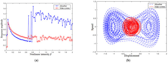
Figure 16.
Response amplitude and phase diagram of two vibrators in the case of off-resonance ω = 1.6. (a) Response amplitude; (b) Phase diagram (β = 0.9).
4.4. Damping Ratio of the Vibration Absorber γ1
Based on the above simulation results, the present parameters are set below. When ω = 1.0, the parameters are set as follows: μ = 0.35, f = 1.5, γ2 = 0.025 and β = 0.8; when ω = 0.6, the parameters are set as follows: μ = 0.3, f = 0.25, γ2 = 0.025 and β = 0.2; when ω = 1.6, the parameters are set as follows: μ = 0.3, f = 1.0, γ2 = 0.025 and β = 0.9.
Figure 17a shows the response amplitude of the main system and the vibration absorber in the case of resonance ω = 1.0. Apparently, when γ1 = 0, the amplitude of the main system and the absorber reached the maximum and then gradually decreased; as the γ1 increased to over 0.025, the amplitude no longer changed. Therefore, the optimal range of γ1 was determined as 0.025–0.50. Figure 17b shows the phase diagram of the main system, when γ1 = 0.05. It is evident that the main system executed slight periodic motion.
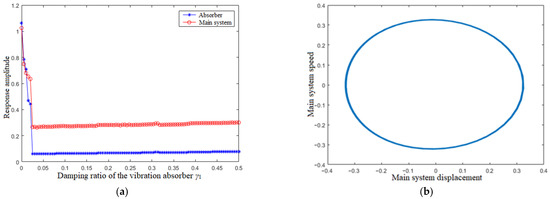
Figure 17.
Response amplitude of two vibrators and phase diagram of main system in the case of resonance ω = 1.0. (a) Response amplitude; (b) Phase diagram (γ1 = 0.05).
Figure 18a shows the response amplitude of two vibrators in the case of off-resonance ω = 0.6. Apparently, the amplitude of the main system was slight and almost remained unchanged, while the amplitude of the absorber reached a maximum at γ1 = 0.01, then gradually decreased and finally converged to a constant value at γ1 > 0.3. Therefore, the optimal damping ratio of the absorber should be set as γ1 = 0.01. Figure 18b shows the phase diagrams of two vibrators. The main system demonstrated small amplitude, while the absorber executed large amplitude.
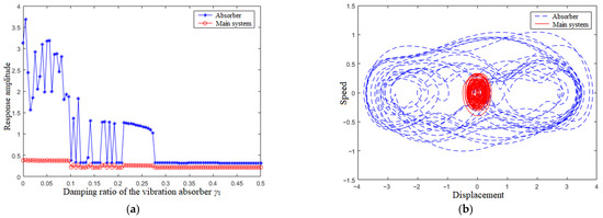
Figure 18.
Response amplitude and phase diagram of two vibrators in the case of off-resonance ω = 0.6. (a) Response amplitude; (b) Phase diagram (γ1 = 0.01).
Figure 19a shows the response amplitude of the main system and the vibration absorber at an excitation frequency ω = 1.6. It can be observed that the amplitude of two vibrators became smoother. The amplitude of the main system was low, while the amplitude of the absorber was high. Accordingly, the optimal damping ratio was determined as γ1 = 0. Figure 19b shows the phase diagrams of two vibrators at γ1 = 0, which show that the absorber executed large amplitude chaotic motion and the main system moved with small amplitude.
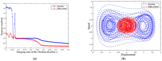
Figure 19.
Response amplitude and phase diagram of two vibrators in the case of off-resonance ω = 1.6. (a) Response amplitude; (b) Phase diagram (γ1 = 0).
5. Conclusions
This study focused on a main system with a bistable vibration absorber to establish the dynamic equations and investigate the dynamic characteristics of the bistable vibration absorber under harmonic excitation. In addition, the effects of the excitation frequency and the excitation amplitude on the system bifurcation and the structural parameters on the bistable absorber’s performance were examined in depth with numerical simulation. The nonlinear vibration absorber can overcome the potential barrier and perform large amplitude chaotic motion at low frequency by analyzing the bifurcation. This contributes to achieving a wider frequency broadband damping effect. Moreover, the performance of the nonlinear vibration absorber is quite sensitive to the change of its own structural parameters. The vibration amplitude of the main system resonance could decrease gradually through structural parameter optimization of the tuning frequency ratio f, the mass ratio μ, the nonlinear intensity β and the damping ratio γ1. In the case of off-resonance, the optimal parameter settings corresponding to the lower amplitude of the main system and the higher amplitude of the vibration absorber can be obtained to improve power generation. The optimal parameter is helpful for improving the performance of the vibration absorber. In the future, the damper can be analyzed on random excitation, which can improve the damping capacity of the vibration absorber under random excitation.
Author Contributions
Conceptualization, Y.L.; methodology, M.Y.; software, J.Z.; validation, Y.L. and X.L.; formal analysis, W.W.; investigation, X.L.; resources, J.Z.; data curation, Y.L. and W.W.; writing—original draft preparation, Y.L.; writing—review and editing, Y.L.; supervision, M.Y.; project administration, X.L; funding acquisition, J.Z. and W.W. All authors have read and agreed to the published version of the manuscript.
Funding
This research was funded by the BJAST Innovation Cultivation Programs, the BJAST Budding Talent Program (BGS202210) and the 2020 Xicheng District Excellent Talents Funding Project.
Institutional Review Board Statement
Not applicable.
Informed Consent Statement
Not applicable.
Data Availability Statement
Data can be obtained from the corresponding author upon reasonable request.
Conflicts of Interest
The authors declare that there is no conflict of interest.
References
- Zhang, M.; Luo, S.; Gao, C.; Ma, W. Research on the mechanism of a newly developed levitation frame with mid-set air spring. Veh. Syst. Dyn. 2018, 56, 1797–1816. [Google Scholar] [CrossRef]
- Zhu, H.; Yang, J.; Zhang, Y.; Feng, X.; Ma, Z. Nonlinear dynamic model of air spring with a damper for vehicle ride comfort. Nonlinear Dyn. 2017, 89, 1545–1568. [Google Scholar] [CrossRef]
- Zhang, W.; Zhao, J. Analysis on nonlinear stiffness and vibration isolation performance of scissor-like structure with full types. Nonlinear Dyn. 2016, 86, 17–36. [Google Scholar] [CrossRef]
- Fiebig, W.; Wróbel, J. Two stage vibration isolation of vibratory shake-out conveyor. Arch. Civ. Mech. Eng. 2017, 17, 199–204. [Google Scholar] [CrossRef]
- Wang, X.; Zhou, J.; Xu, D.; Ouyang, H.; Duan, Y. Force transmissibility of a two-stage vibration isolation system with quasi-zero stiffness. Nonlinear Dyn. 2017, 87, 633–646. [Google Scholar] [CrossRef]
- Beijen, M.A.; Heertjes, M.F.; Butler, H.; Steinbuch, M. Disturbance feedforward control for active vibration isolation systems with internal isolator dynamics. J. Sound Vib. 2018, 436, 220–235. [Google Scholar] [CrossRef]
- Melik-Shakhnazarov, V.A.; Strelov, V.I.; Sofiyanchuk, D.V.; Tregubenko, A.A. Active vibration isolation devices with inertial servo actuators. Cosm. Res. 2018, 56, 140–143. [Google Scholar] [CrossRef]
- Virgin, L.N.; Santillan, S.T.; Plaut, R.H. Vibration isolation using extreme geometric nonlinearity. J. Sound Vib. 2008, 315, 721–731. [Google Scholar] [CrossRef]
- Guest, S.D.; Pellegrino, S. Analytical models for bistable cylindrical shells. Proc. R. Soc. A 2006, 462, 839–854. [Google Scholar] [CrossRef]
- Zhao, T.Y.; Ma, Y.; Zhang, H.Y.; Pan, H.G.; Cai, Y. Free vibration analysis of a rotating graphene nanoplatelet reinforced pre-twist blade-disk assembly with a setting angle. Appl. Math. Model. 2021, 93, 578–596. [Google Scholar] [CrossRef]
- Zhao, T.Y.; Cui, Y.S.; Pan, H.G.; Yuan, H.Q.; Yang, J. Free vibration analysis of a functionally graded graphene nanoplatelet reinforced disk-shaft assembly with whirl motion. Int. J. Mech. Sci. 2021, 197, 106335. [Google Scholar] [CrossRef]
- Zhao, T.Y.; Yan, K.; Li, H.W.; Wang, X. Study on theoretical modeling and vibration performance of an assembled cylindrical shell-plate structure with whirl motion. Appl. Math. Model. 2022, 110, 618–632. [Google Scholar] [CrossRef]
- Nicassio, F. Shape prediction of bistable plates based on Timoshenko and Ashwell theories. Compos. Struct. 2021, 265, 113645. [Google Scholar] [CrossRef]
- Kremer, D.; Liu, K. A nonlinear energy sink with an energy harvester: Transient responses. J. Sound Vib. 2014, 333, 4859–4880. [Google Scholar] [CrossRef]
- Kremer, D.; Liu, K. A nonlinear energy sink with an energy harvester: Harmonically forced responses. J. Sound Vib. 2017, 410, 287–302. [Google Scholar] [CrossRef]
- Peng, Y.; Liu, J. Modeling and vibration control for a flexible pendulum inverted system based on a PDE observer. Int. J. Control 2016, 90, 1736–1751. [Google Scholar] [CrossRef]
- Sun, C.; Jahangiri, V.; Sun, H. Performance of a 3D pendulum tuned mass damper in offshore wind turbines under multiple hazards and system variations. Smart Struct. Syst. 2019, 24, 53–65. [Google Scholar]
- Taghipour, J.; Dardel, M.; Pashaei, M.H. Vibration mitigation of a nonlinear rotor system with linear and nonlinear vibration absorbers. Mech. Mach. Theory 2018, 128, 586–615. [Google Scholar] [CrossRef]
- Stanton, S.C.; Culver, D.; Mann, B.P. Tuning inertial nonlinearity for passive nonlinear vibration control. Nonlinear Dyn. 2020, 99, 495–504. [Google Scholar] [CrossRef]
- Shui, X.; Wang, S. Investigation on a mechanical vibration absorber with tunable piecewise-linear stiffness. Mech. Syst. Signal Process. 2018, 100, 330–343. [Google Scholar] [CrossRef]
- Yan, L.; Gong, X. Experimental study of vibration isolation characteristics of a geometric anti-spring isolator. Appl. Sci. 2017, 7, 711. [Google Scholar] [CrossRef]
- Shapiro, B.; Kissel, J.; Mavalvala, N.; Strain, K.; Youcef-Toumi, K. Limitations of underactuated modal damping for multistage vibration isolation systems. IEEE-ASME Trans. Mech. 2014, 20, 393–404. [Google Scholar] [CrossRef]
- Tuna, M.; Kirca, M. Exact solution of Eringen’s nonlocal integral model for vibration and buckling of Euler–Bernoulli beam. Int. J. Eng. Sci. 2016, 107, 54–67. [Google Scholar] [CrossRef]
- Zheng, Y.; Zhang, X.; Luo, Y.; Yan, B.; Ma, C. Design and experiment of a high-static–low-dynamic stiffness isolator using a negative stiffness magnetic spring. J. Sound Vib. 2016, 360, 31–52. [Google Scholar] [CrossRef]
- Zhao, T.Y.; Jiang, L.P.; Pan, H.G.; Yang, J.; Kitipornchai, S. Coupled free vibration of a functionally graded pre-twisted blade-shaft system reinforced with graphene nanoplatelets. Compos. Struct. 2021, 262, 113362. [Google Scholar] [CrossRef]
- Zhao, T.Y.; Li, K.; Ma, H. Study on dynamic characteristics of a rotating cylindrical shell with uncertain parameters. Anal. Math. Phys. 2022, 12, 97. [Google Scholar] [CrossRef]
- Yan, W.; Yu, Y.; Mehta, A. Analytical modeling for rapid design of bistable buckled beams. Theor. Appl. Mech. Lett. 2019, 9, 264–272. [Google Scholar] [CrossRef]


Disclaimer/Publisher’s Note: The statements, opinions and data contained in all publications are solely those of the individual author(s) and contributor(s) and not of MDPI and/or the editor(s). MDPI and/or the editor(s) disclaim responsibility for any injury to people or property resulting from any ideas, methods, instructions or products referred to in the content. |
© 2023 by the authors. Licensee MDPI, Basel, Switzerland. This article is an open access article distributed under the terms and conditions of the Creative Commons Attribution (CC BY) license (https://creativecommons.org/licenses/by/4.0/).