Automation of Experimental Modal Analysis Using Bayesian Optimization

Abstract

The dynamic characterization of structures by means of modal parameters offers many valuable insights into the vibrational behavior of these structures. However, modal parameter estimation has traditionally required expert knowledge and cumbersome manual effort such as, for example, the selection of poles from a stabilization diagram. Automated approaches which replace the user inputs with a set of rules depending on the input data set have been developed to address this shortcoming. This paper presents an alternative approach based on Bayesian optimization. This way, the possible solution space for the modal parameter estimation is kept as widely open as possible while ensuring a high accuracy of the final modal model. The proposed approach was validated on both a synthetic test data set and experimental modal analysis data of a machine tool. Furthermore, it was benchmarked against a similar tool from a well-known numerical computation software application.

1. Introduction

The vibrational characteristics of structures represent one of the key design targets in mechanical, aerospace, and civil engineering, as well as in many other domains. Typically, the dynamic behavior is described by a linear model which relates time-varying input forces on the structure of interest to its (also time-varying) displacements [1]. Most often, modal models which are based on the so-called modal parameters eigenfrequencies, mode shapes, and modal damping are used due to their intuitive physical interpretability [2]. In this context, one also speaks of poles containing the combined information of eigenfrequency and modal damping. Building up and evaluating these models is, depending on the chosen approach, either called computational or experimental modal analysis (EMA). Even though simulations have improved in recent years, real-world experiments are still needed in cases in which high accuracy is essential, or in order to calibrate the computational analyses, as, for example, demonstrated by Ellinger and Zaeh [3]. EMA is typically performed under laboratory conditions [4], which may not be sufficient for capturing the vibrational characteristics of a generally nonlinear system using the linear modal model. In contrast, operational modal analysis (OMA) is performed under operational conditions, an approach which is typically more accurate but comes with additional challenges such as only partial or missing input force measurements [4].

Given a set of data, a variety of methods exists for estimating the modal parameters of a system. In case the modes are identified one at a time rather than all at once, they are called single-degree-of-freedom methods [5]. Popular examples include the peak-picking, the circle-fit, and the line-fit methods [5], as well as the two-stage least squares identification presented by Altintas [6]. When dealing with closely spaced modes, so-called multi-degree-of-freedom (MDOF) methods, which consider multiple modes simultaneously, typically perform better [5]. This can, for example, be done by solving a nonlinear optimization problem [5,6], the global rational fraction polynomial method [5], the least squares rational function (LSRF) method [7], global singular value decomposition (SVD) [5], the least squares complex exponential (LSCE) method [8], the least squares complex frequency-domain (LSCF) method or its polyreference version, the so called "PolyMAX" method [9], or various stochastic subspace identification (SSI) methods [10]. Depending on whether they operate on time series or frequency information, these algorithms can either be clustered as time-domain (e.g., SSI or the LSCE method) or frequency-domain (e.g., the circle-fit method, global SVD, or the LSCF method) approaches.

The algorithms themselves are beyond the scope of this paper. However, all approaches have in common that the model order must be set, which directly relates to the question of how many modes are to be identified. Although strategies exist for determining a suitable model order based on the measured data, it is more common to first considerably overestimate the number of modes and identify modal parameters for several model orders and, second, to select an appropriate number of modes based on the combined information [4,5]. This approach helps to reduce biases in the identified modes [4]. However, when proceeding in this way, many spurious or mathematical modes occur which must be separated from the true, physical modes. The central element of this strategy is the so-called stabilization diagram, which displays the identified modes in a model order over frequency plot [4].

In the past, selecting appropriate modes from the stabilization diagram has required a high level of user interaction and expert knowledge [11,12]. To simplify the process, Scionti et al. [13] first made use of several methods to eliminate spurious modes applicable to state spaced models and, second, introduced a set of rules to mimic the selection of modes by the user. The rules depend on several parameters, for which default values were set. They found that the proposed approach performs well on in-flight flutter data for an aircraft. A short review on such mode separation rules, which, in the end, emulate the actions and decisions of an experienced user, was provided by van der Auweraer and Peeters [14]. The latter further mentioned in-flight data analysis and structural health monitoring as possible applications. Their work was extended by Lau et al. [1], who also referred to Scionti et al. [13] by developing a rule-based automatic modal parameter selection approach. Peer group comparisons between modal analysis novices and experts on two comprehensive data sets proved that the approach leads to skill-independent results and an overall productivity gain of 50%.

A different approach was followed by Scionti and Lanslots [11], who compared several Fuzzy c-means clustering techniques with and without an additional genetic algorithm (GA) for the initialization of finding pole candidates. It was found that the Gustafson–Kessel algorithm with initial values from a GA resulted in the best clusters of poles. Some clusters were immediately discarded based on their contribution ratio, their compactness measures, and corresponding thresholds. For each remaining cluster, the pole closest to its center was chosen as the final result, which was positively evaluated by comparing it to the poles found by experts.

All of the works presented still rely on user-defined thresholds and are thus not fully automated [12]. This drawback was overcome by Reynders et al. [12], who, in addition to a very comprehensive literature review, proposed a three-stage approach for fully automated modal parameter estimation. First, all modes were classified as either spurious or potentially stable by eleven soft and three hard validation criteria. Second, the remaining poles were hierarchically clustered to find similar modes and, finally, the mode with a modal damping closest to the median damping of the corresponding cluster was selected. The approach was successfully tested on several data sets. However, the results were only benchmarked against modal parameters retrieved by a manual analysis. A comparison of the modal model with the original data set was not performed. A very similar strategy was followed by Neu et al. [15]. However, the latter allowed larger damping values, used different features representing the soft validation criteria, and selected the final poles by averaging all pole candidates per cluster. Additionally, they examined the influence of the maximum model order and found that their approach was less sensitive to it than that by Reynders et al. [12]. The method was applied to an OMA data set and successfully compared to EMA and finite element analysis results. Mugnaini et al. [16] proposed slight adaptations to the approach of Neu et al. [15] and proved their effectiveness in an ablation study for a helicopter blade data set. Additionally, the eigenfrequency identification was validated on a simulated data set. Again, no validation against the original data set was conducted in Neu et al. [15] and Mugnaini et al. [16].

It can be concluded that a consensus has been formed in the state-of-the-art regarding the basic approach of automatically extracting modal parameters [12,15,16]. However, it was not evaluated how well the identified modal model replicates the original data set using, for example, the frequency response assurance criterion (FRAC), nor was this the focus of the modal parameter extraction. Furthermore, the parameters which required user input in earlier approaches [1,11,13,14] were replaced by metrics performed on the input data set [12,15,16], which is believed to unnecessarily restrict the solution space for the final modal parameters. The present paper presents an alternative approach, in which Bayesian optimization is used to find the optimal values of any required hyperparameters. The deviation between the identified modal model and the original data set is used as a cost function. This also ensures a high level of validity for the final modal model.

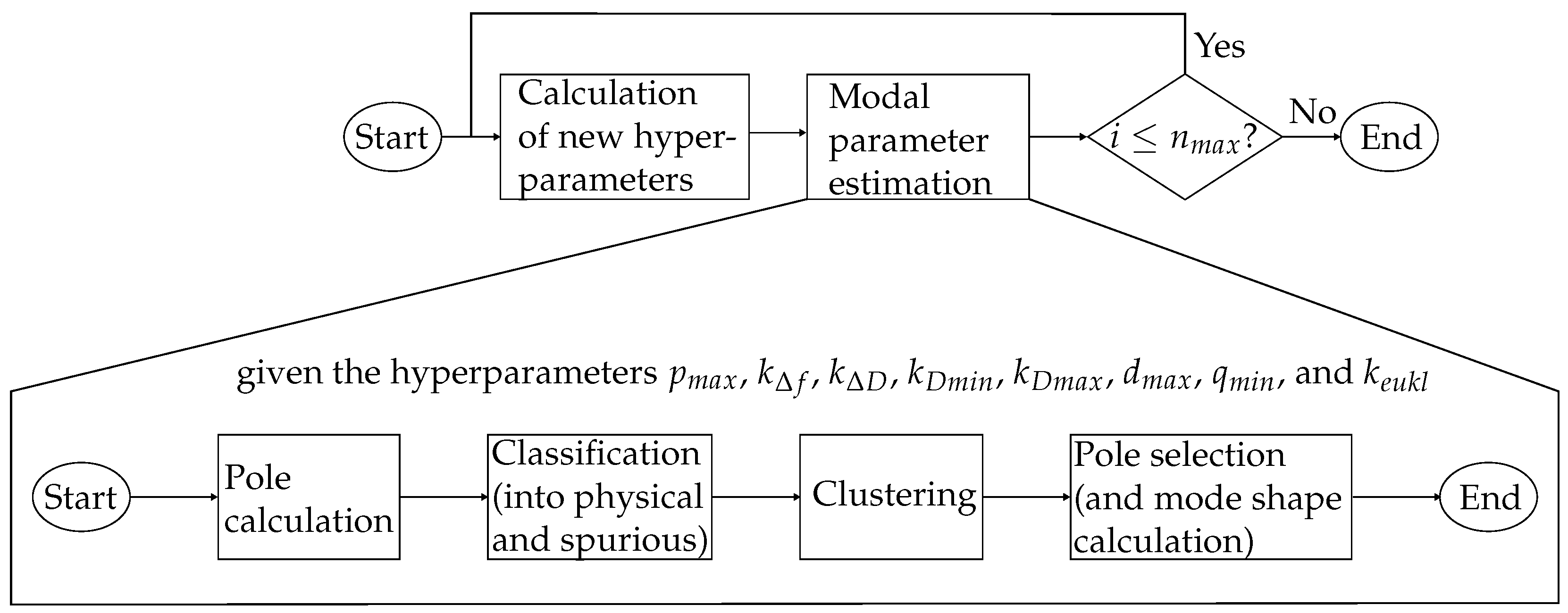
The remainder of this paper is structured as follows: Section 2 presents the proposed approach in general. It will be shown how modal parameters are extracted based on a few hyperparameters, which will subsequently be optimized using a Bayesian optimization approach. Section 3, on the one hand, validates the proposed approach on a synthetic test data set. On the other hand, modal parameters were extracted from input data measured on a machine tool. Additionally, the results from both data sets were benchmarked against the MATLAB^® function modalfit. Last, Section 4 summarizes the main content of the paper and offers an outlook to future research.

2. Proposed Method

This section presents a new approach for modal parameter estimation, which will be called AutoEMA. In contrast to the recent literature [12,15,16], hyperparameters are not automatically derived from the input data set, but rather set by a Bayesian optimization algorithm such that the match between the identified modal model and the original input data is as high as possible. Section 2.1 describes in detail how modal parameters are extracted based on (measured) input data and a set of hyperparameters. Section 2.2 demonstrates how values for these hyperparameters can be found such that the modal parameters and the corresponding modal model optimally represent the original input data. Figure 1 illustrates the overall approach.

2.1. Modal Parameter Estimation

The first step is calculating pole candidates for all model orders $p_i=1,2,\dots ,p_{max}$ up to and including the maximum model order $p_{max}$. In the present research, this is done using the PolyMAX algorithm [9], but a variety of other methods are also applicable (see Section 1). The found pole candidates are then classified as certainly spurious and potentially physical by applying four criteria: The relative difference in frequency of a pole of order $p_i$ to any pole of model order $p_{i-1}$ must be smaller than $k_{\mathrm{\Delta }f}$ (a), the relative difference in damping of a pole of order $p_i$ to any pole of model order $p_{i-1}$ must be smaller than $k_{\mathrm{\Delta }D}$ (b), and the pole’s damping must be larger than $k_{Dmin}$ (c) and smaller than $k_{Dmax}$ (d). If all conditions (a) to (d) for a given pole are met, it is classified as potentially physical, otherwise as certainly spurious. Figure 2 exemplarily shows the frequency of all potentially physical poles of a given frequency response function (FRF).

Spurious poles are discarded and thus excluded from further analysis. Given that many model orders were considered, there are generally several remaining poles for any mode shape being identified. Agglomerative clustering is used to group poles into modes. Given that this is a hierarchical clustering algorithm, the algorithm determines the number of clusters. However, a threshold has to be set, in this case the maximum frequency distance of poles within a cluster $d_{max}$. If the clustering is applied to the poles in Figure 2, six possible modes are found, as illustrated in Figure 3.

Two more rules were applied in order to avoid clusters having spurious poles only. First, it was assumed that clusters reflecting actual modes contain at least a certain percentage of the model order p${}_i$ of poles, in this case $q_{min}$. This rule directly corresponds to the original assumption that physical poles show up at many model orders [14]. Second, the variance in frequency of poles of spurious-only clusters is assumed to be higher than the one from a cluster reflecting an actual mode. Thus, all clusters with an average Euclidean distance larger than $k_{eukl}·d_{max}$ are discarded, where $d_{max}$ is the maximum frequency distance of poles within a cluster from the clustering stage and $k_{eukl}$ is an euclidean frequency distance factor.

Finally, one pole per cluster can be selected by choosing the pole closest to the median pole location of a cluster, which is indicated by crosses in Figure 3. The pole determines both eigenfrequency and modal damping of the mode corresponding to the cluster. After all poles have been selected, the mode shapes are calculated using the least squares frequency-domain method [9].

Table 1. Overview of hyperparameters used in the modal parameter estimation; the classification parameters are defined similar to Reynders et al. [12] and Neu et al. [15].

Step	Symbol	Description
Pole calculation	$p_{max}$	Maximum model order
Classification	$k_{\mathrm{\Delta }f}$	Maximum relative frequency difference of two poles
	$k_{\mathrm{\Delta }D}$	Maximum relative damping difference of two poles
	$k_{Dmin}$	Minimum damping of a mode
	$k_{Dmax}$	Maximum damping of a mode
Clustering	$d_{max}$	Maximum frequency distance within a cluster
	$q_{min}$	Minimum percentage of the model order of poles per cluster
	$k_{eukl}$	Maximum euclidean frequency distance factor between poles
Pole selection	-	-

summarizes the hyperparameters involved in the modal parameter estimation. The code used in this work is based on the Python package pyEMA [17].

2.2. Hyperparameter Optimization

The modes identified and the corresponding modal parameters strongly depend on the hyperparameters used in the modal parameter estimation step (see Table 1). The key idea behind this publication is to find optimal values for these parameters, whereas the recent literature has dealt with deriving them based on the input data set [12,15,16]. On the one hand, the presented approach keeps the solution space as widely open as possible. On the other hand, it ensures a high concordance between the original input data and the resulting modal model. A variety of optimization algorithms exist in the literature. The decision on which depends, amongst others, on the amount of knowledge on the system being optimized, the availability of efficient gradient calculations, and the shape as well as the (computation) costs of evaluating the objective function. The specific objective function used will be described below and will involve running the modal parameter estimation (see Section 2.1). As the relationship between the hyperparameters and the resulting modal parameters is rather complex, no gradients are available since $p_{max}$ is a discrete number, the objective function is generally non-convex, and the costs of evaluating the objective function can be high (depending on the chosen maximum model order $p_{max}$ and the size of the input FRF data set), the Bayesian optimization approach was chosen here [18]. In the context of this method, the objective function is generally treated as random and approximated with a Gaussian process regression model. Previous objective function evaluations are treated as prior knowledge and are considered as a prior. New function evaluations increase the knowledge about the objective function, which is then used to update the prior, forming the so-called posterior. The posterior, in turn, can then be used in several ways to determine the location of further new, promising function evaluations. Those locations are determined with the help of an acquisition function. In this case, the so-called upper confidence bound optimization policy was applied, allowing the balance between exploitation and exploration to be easily set. A comprehensive guide on Bayesian optimization can be found in Garnett [18].

The AutoEMA method tries to find values for the hyperparameters (see Table 1) such that the identified modal parameters and the corresponding modal model best replicate the original input data, which is given in the form of FRFs. To measure the match between two FRFs, the FRAC can be used:

$$\begin{array}{cc}\hfill \mathrm{F}\mathrm{R}\mathrm{A}\mathrm{C}({\mathit{H}}_1\left(\omega \right),{\mathit{H}}_2\left(\omega \right))& =\frac{|{\mathit{H}}_1{\left(\omega \right)}^T{\mathit{H}}_2^{*}{\left(\omega \right)|}^2}{\left({\mathit{H}}_1{\left(\omega \right)}^T{\mathit{H}}_1^{*}\left(\omega \right)\right)\left({\mathit{H}}_2{\left(\omega \right)}^T{\mathit{H}}_2^{*}\left(\omega \right)\right)},\hfill \end{array}$$

(1)

where ${\mathit{H}}_1\left(\omega \right)$ and ${\mathit{H}}_2\left(\omega \right)$ are the FRFs being compared, $\omega$ is the angular frequency, and ${\mathit{x}}^{*}$ is the complex conjugation and ${\mathit{x}}^T$ the transpose of a vector $\mathit{x}$ [19]. FRAC values of 100% indicate a perfect match, whereas values of 0% mean no correlation at all.

An average value over all input FRFs is computed to assess the complete input data set:

$$\begin{array}{c}\hfill \overline{\mathrm{F}\mathrm{R}\mathrm{A}\mathrm{C}}=\frac{1}{n_{inp}}\sum _{k=1}^{n_{inp}}\mathrm{F}\mathrm{R}\mathrm{A}\mathrm{C}({\mathit{H}}_{inp,k},{\mathit{H}}_{model,k})\end{array}$$

(2)

In this case, $n_{inp}$ is the number of input FRFs, ${\mathit{H}}_{inp,k}$ are the original input FRFs, and ${\mathit{H}}_{model,k}$ are the FRFs resulting from the modal model. Note that the angular frequency $\omega$ has been dropped for the sake of readability. The concordance between the model FRFs and the input FRFs generally increases with an increasing number of modes in the model. To prevent spurious modes approximating noise in the measurement data, Equation (2) is extended by a (small) regularization parameter r, which penalizes a high number of found modes number of modes ($n_{modes}$):

$$\begin{array}{c}\hfill y=\overline{\mathrm{F}\mathrm{R}\mathrm{A}\mathrm{C}}-n_{modes}r\end{array}$$

(3)

The final optimization cost function y can then be constructed by combining Equations (1)–(3), with ${\mathit{H}}_{model,k}$ in Equation (2) being a function of the hyperparameters to be optimized:

$$\begin{array}{c}\hfill {\mathit{H}}_{model,k}=f(k,p_{max},k_{\mathrm{\Delta }f},k_{\mathrm{\Delta }D},k_{Dmin},k_{Dmax},d_{max},q_{min},k_{eukl})\end{array}$$

(4)

As shown in Figure 1, the Bayesian optimization is terminated when the current iteration number i exceeds the set maximum iteration number $n_{max}$.

3. Application

In this section, the application of the approach presented in Section 2 is described for two use cases: First, synthetic test data were simulated using a sixth-order MDOF oscillator model (see Section 3.1). In this case, the ground truth values of the modal parameters were known per definition, and their estimated values could be directly compared to their reference values. Artificial noise was superimposed to show the robustness of the proposed approach. Second, data measured on a real-world machine tool test bench were used as input for the automated modal parameter estimation approach (see Section 3.2). In both cases, the resulting modal parameters were benchmarked against the function modalfit from the signal processing toolbox of the well-established numerical computation program MATLAB^®.

3.1. Synthetic Test Data

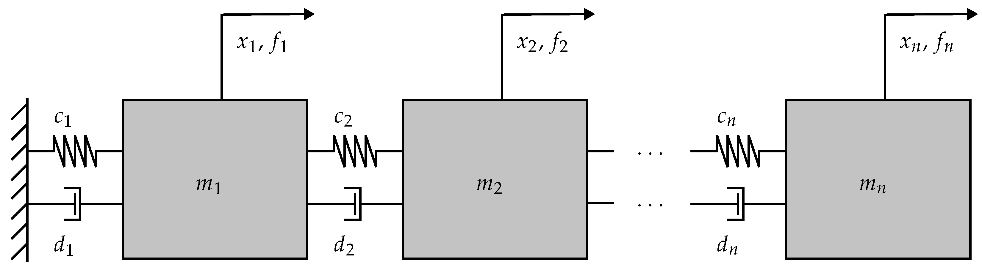
To test the proposed approach, an oscillator with six degrees of freedom (DOFs) was set up as shown in Figure 4 and used for simulating synthetic reference input data. Using a time-domain simulation, six FRFs were calculated from an input force at the first mass $f_1$ to the displacement at all DOFs. To demonstrate the robustness of the AutoEMA method, normal (Gaussian) noise with zero mean was superimposed to the respective outputs $x_1,x_2,\dots ,x_6$. Additionally, the (damped) eigenvalue problem was solved, resulting in estimates for the mode shapes, the eigenfrequencies, and the modal damping ratios. These modal parameters are, in the following, regarded as ground truth values and to be estimated using both the MATLAB^® and the AutoEMA approach.

Regarding the AutoEMA approach,

Table 2. Value range and initial values of the hyperparameters used in the optimization stage of the modal parameter optimization for both use cases; a description of the parameters can be found in Table 1 and Section 2.1. The regularization parameter r and the minimum modal damping $k_{Dmin}$ were set constant.

Hyperparameter	Initial Value	Value Range
$p_{max}$	80	60 to 120
$k_{\mathrm{\Delta }f}$	1%	0.1% to 10%
$k_{\mathrm{\Delta }D}$	5%	5% to 20%
$k_{Dmin}$	0%
$k_{Dmax}$	20%	20% to 30%
$d_{max}$	2 $\mathrm{Hz}$	0.4 $\mathrm{Hz}$ to 4 $\mathrm{Hz}$
$q_{min}$	30%	20% to 60%
$k_{eukl}$	0.5	0.1 to 0.8
r	0.002

shows the value range constraining the hyperparameters of the modal parameter estimation in the Bayesian optimization process and their initial values. These boundaries were considered to be wide in order to keep the solution space as widely open as possible. Note that the minimum damping of a mode $k_{Dmin}$ was set to the lowest physically meaningful value of 0%, so it was excluded from the optimization in this case. Per definition, the regularization parameter r cannot be optimized and was also fixed. However, the value r of $0.002$ has been found to be suitable for many data sets, including the one used herein and the real-world data shown in Section 3.2. The initial values were chosen arbitrarily within the bounds, as the result of the Bayesian optimization was found to be widely insensitive. In total, 40 iterations, that is, evaluations of the cost function (see Section 2.2), were made.

The same data were also fed into the MATLAB^® function modalfit. It requires the number of modes to be determined as an input parameter. In this case, it was set to the true value of six modes, which was also identified automatically by the AutoEMA approach. The modalfit function has implemented both the LSCE and the LSRF algorithms. Here, the default LSCE method was used.

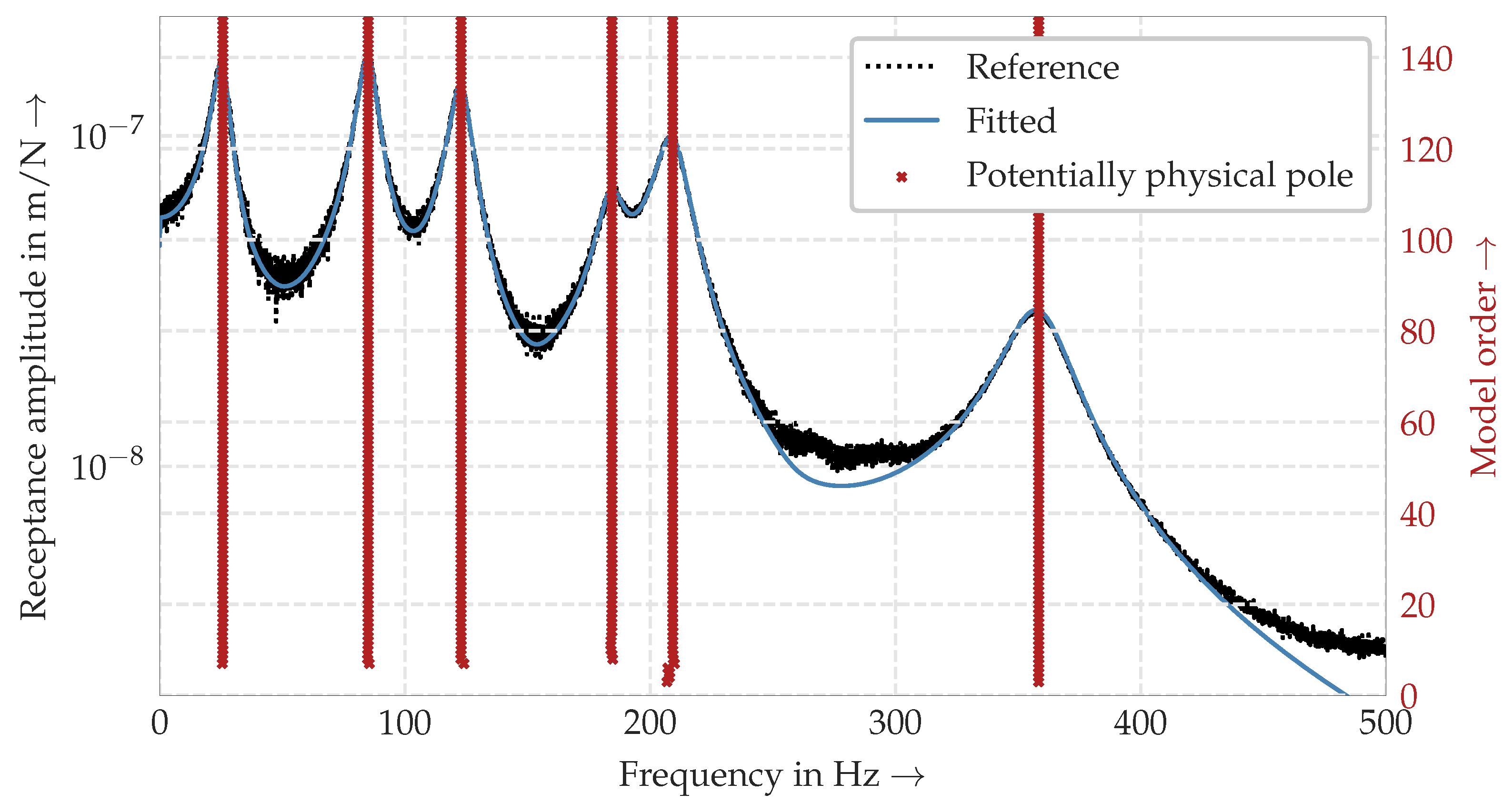
Figure 5 shows the (simulated) reference FRF from a force input $f_1$ at the first DOF to the displacement $x_1$ at the same DOF alongside the reconstructed FRFs from both the MATLAB^® and AutoEMA modal models. It can be seen that both approaches estimated the original FRF well despite the presence of noise. However, the AutoEMA approach slightly outperformed the MATLAB^® approach in the low frequency region up to 150 $\mathrm{Hz}$.

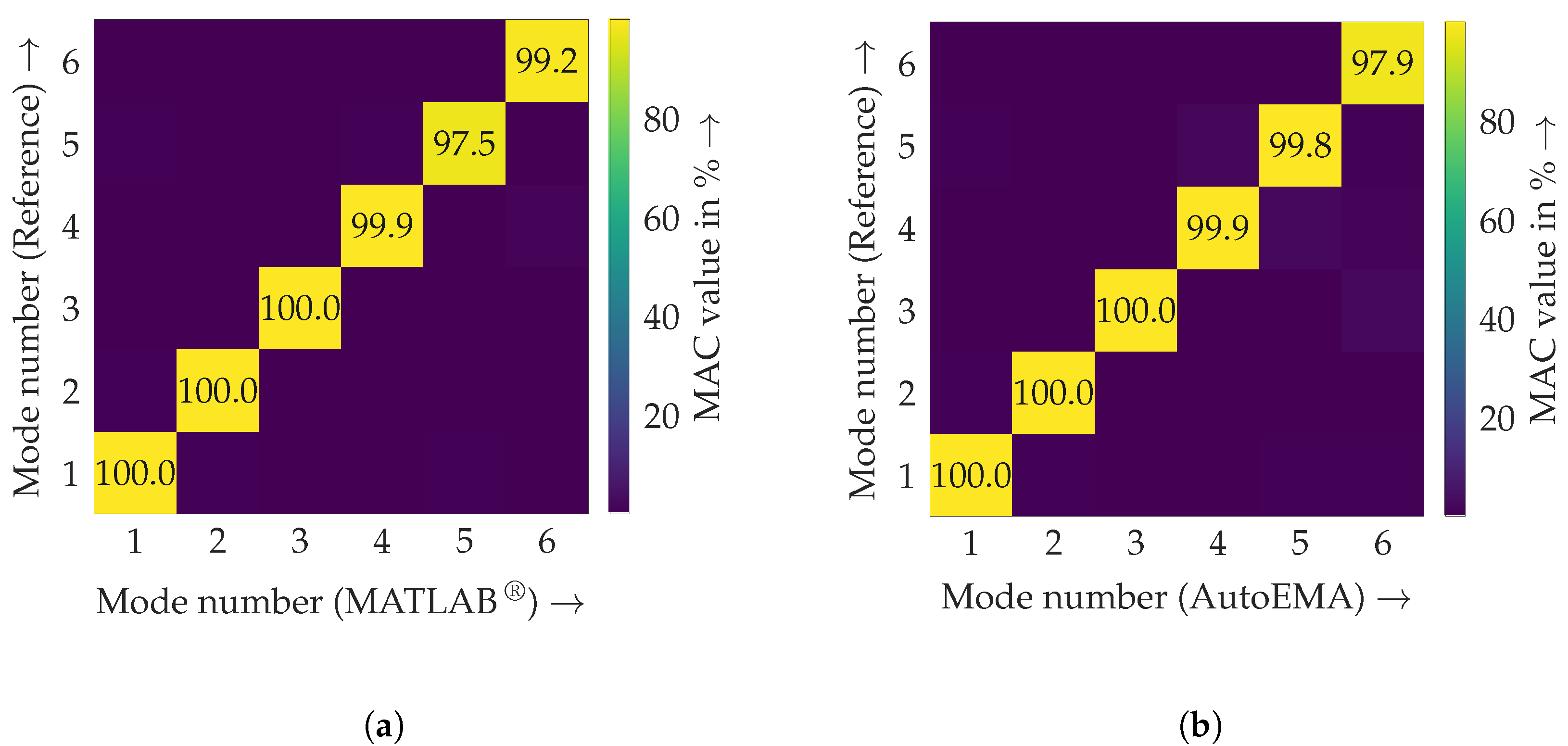
Figure 6 shows the conformance of the estimated mode shapes with the (simulated) reference data quantified by the modal assurance criterion (MAC) [20], which is defined as

$$\begin{array}{cc}\hfill \mathrm{M}\mathrm{A}\mathrm{C}({\mathbf{\phi }}_1,{\mathbf{\phi }}_2)& =\frac{|{\mathbf{\phi }}_1^T{\mathbf{\phi }}_2^{*}{|}^2}{\left({\mathbf{\phi }}_1^T{\mathbf{\phi }}_1^{*}\right)\left({\mathbf{\phi }}_2^T{\mathbf{\phi }}_2^{*}\right)}.\hfill \end{array}$$

(5)

In this case, ${\mathbf{\phi }}_i$ are mode shapes being compared, and, again, ${\mathit{x}}^{*}$ denotes the complex conjugation and ${\mathit{x}}^T$ the transpose of a vector $\mathit{x}$. Similar to the FRAC, a value of 0% indicates no correlation at all, and a result of 100% states a perfect coincidence between the two mode shapes. It can be seen that both approaches estimated the reference mode shapes equally well with very high concordance.

To assess the accuracy of eigenfrequencies $f_i^e$, the natural frequency difference (NFD) criterion can be used [21]:

$$\begin{array}{c}\hfill \mathrm{N}\mathrm{F}\mathrm{D}(f_1^e,f_2^e)=\frac{|f_1^e-f_2^e|}{min\left(f_1^e,f_2^e\right)}\end{array}$$

(6)

By slightly adapting Equation (6), a similar comparison can be made regarding the modal damping ratios ${\xi }_i$ using the natural damping difference (NDD):

$$\begin{array}{c}\hfill \mathrm{N}\mathrm{D}\mathrm{D}({\xi }_1,{\xi }_2)=\frac{|{\xi }_1-{\xi }_2|}{min\left({\xi }_1,{\xi }_2\right)}\end{array}$$

(7)

Both criteria indicate perfect coincidence with a value of 0% and increase with a rising difference between the damping ratios and eigenfrequencies to be compared, respectively.

Table 3. Overview of the eigenfrequency results for the synthetic data use case (see Section 3.1) showing the absolute values and the NFD for both the MATLAB^® (ML) and AutoEMA (AE) approach.

Mode	${\mathit{\omega }}_{\mathit{ref}}$	${\mathit{\omega }}_{\mathit{ML}}$	${\mathit{\omega }}_{\mathit{AE}}$	${\mathbf{NFD}}_{\mathit{ref}-\mathit{ML}}$	${\mathbf{NFD}}_{\mathit{ref}-\mathit{AE}}$
1	33.8 Hz	33.8 Hz	33.7 Hz	0.0%	0.2%
2	86.6 Hz	86.6 Hz	86.6 Hz	0.0%	0.0%
3	186.7 Hz	186.6 Hz	186.6 Hz	0.0%	0.0%
4	237.3 Hz	236.6 Hz	237.3 Hz	0.3%	0.0%
5	250.5 Hz	250.3 Hz	250.5 Hz	0.1%	0.0%
6	318.9 Hz	318.4 Hz	319.5 Hz	0.1%	0.2%

and

Table 4. Overview of the modal damping results for the synthetic data use case (see Section 3.1) showing the absolute values and the NDD for both the MATLAB^® (ML) and AutoEMA (AE) approach.

Mode	${\mathit{\xi }}_{\mathit{ref}}$	${\mathit{\xi }}_{\mathit{ML}}$	${\mathit{\xi }}_{\mathit{AE}}$	${\mathbf{NDD}}_{\mathit{ref}-\mathit{ML}}$	${\mathbf{NDD}}_{\mathit{ref}-\mathit{AE}}$
1	$11.4$%	$11.3$%	10%	$0.7$%	$13.9$%
2	$5.0$%	$5.0$%	$4.8$%	$0.3$%	$3.9$%
3	$3.4$%	$3.4$%	$3.4$%	$0.2$%	$0.1$%
4	$3.3$%	$3.6$%	$3.3$%	$8.6$%	$0.6$%
5	$3.3$%	$3.4$%	$3.2$%	$4.4$%	$1.9$%
6	$3.5$%	$3.7$%	$3.0$%	$6.1$%	$17.1$%

show these criteria along with the absolute values for the synthetic data use case. Again, it can be seen that both approaches estimated the reference modal damping ratios and eigenfrequencies well with maximum deviations of $0.3$% and $17.1$% of the NFD and NDD, respectively.

3.2. Machine Tool Data

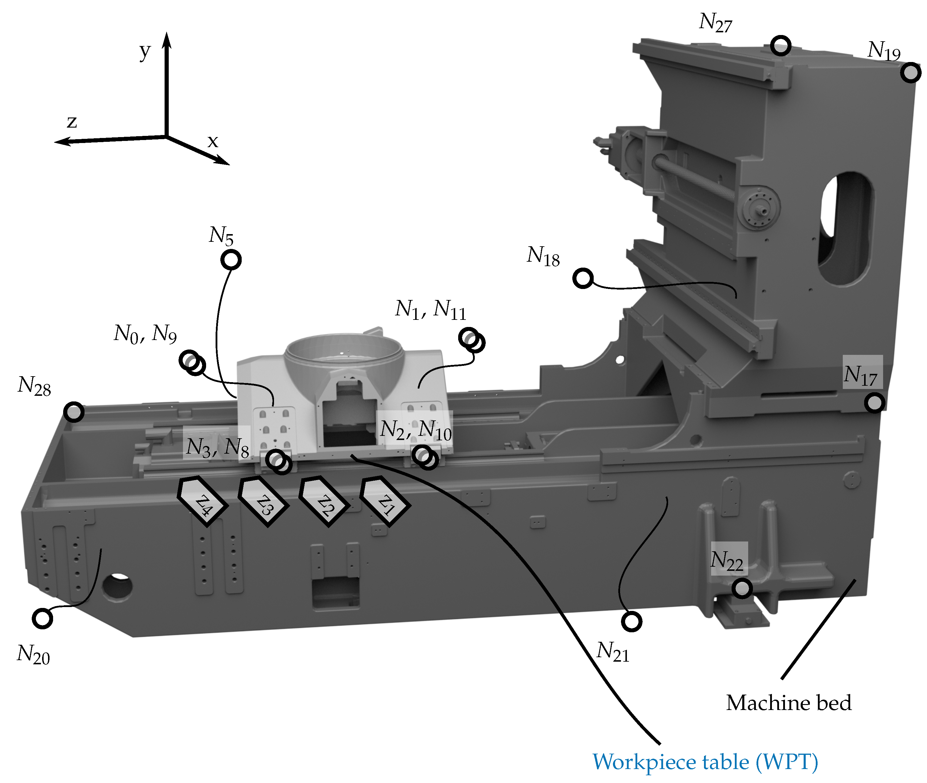
A second data set was acquired on a DMG DMC duo Block 55H machine tool in order to demonstrate the robustness and effectiveness of the proposed modal parameter extraction method (i.e., the AutoEMA method). As illustrated in Figure 7, the machine tool consists of a machine tool bed and a workpiece table (WPT), enabling movement in the global z-axis.

The machine tool’s vibrational response was measured at 17 nodes in all three spatial directions. Four Kistler^® triaxial accelerometers (two times type 8762A10 and two times type 8762A50) were used together with a National Instruments (NI)^® cDAQ-9198 rack with three type NI^®-9232 modules and one type NI^®-9234 module. The measurements were repeated for four WPT positions z${}_1$, z${}_2$, z${}_3$, and z${}_4$ along the z-axis with impulse hammer excitations in x-, y-, and z-directions. The node points are shown in Figure 7 and described in

Table 5. Model nodes considered; the node locations are illustrated in Figure 7.

Node	Description
N${}_0$, N${}_9$	Shoe and rail nodes of the first LGS shoe
N${}_1$, N${}_{11}$	Shoe and rail nodes of the second LGS shoe
N${}_2$, N${}_{10}$	Shoe and rail nodes of the third LGS shoe
N${}_3$, N${}_8$	Shoe and rail nodes of the fourth LGS shoe
N${}_5$	WPT node
N${}_{17}$, N${}_{18}$, N${}_{19}$, N${}_{27}$	Machine bed nodes
N${}_{20}$, N${}_{21}$, N${}_{22}$	ME nodes
N${}_{28}$	Excitation node

. In particular, a corner of the machine tool bed ($N_{28}$) was chosen as the excitation node. For each WPT position, the data acquisition has resulted in 153 FRFs (17 nodes measured in three spatial directions for three excitation directions). The FRFs were calculated as the average of three hammer hits for a measurement duration of 4 $\mathrm{s}$ with a sampling rate of 10,240 $\mathrm{Hz}$.

The approach presented in Section 2 was applied for each WPT position using the same parameter bounds as in the synthetic data use case (see Table 2). Because of the more complicated structure, the optimization was stopped after 100 iterations in this case.

Table 6. Found values of the hyperparameters (see Table 1) in the Bayesian optimization step for different WPT positions.

	${\mathit{p}}_{\mathit{max}}$	${\mathit{k}}_{\mathbf{\Delta }\mathit{f}}$	${\mathit{k}}_{\mathbf{\Delta }\mathit{D}}$	${\mathit{k}}_{\mathit{D}\mathit{max}}$	${\mathit{d}}_{\mathit{max}}$	${\mathit{q}}_{\mathit{min}}$	${\mathit{k}}_{\mathit{eukl}}$
z${}_1$	108	4.2%	15.1%	25.6%	0.20 $\mathrm{Hz}$	27.9%	0.50
z${}_2$	108	5.9%	6.9%	21.7%	0.52 $\mathrm{Hz}$	28.8%	0.61
z${}_3$	108	0.4%	6.2%	24.0%	0.36 $\mathrm{Hz}$	28.6%	0.55
z${}_4$	112	5.4%	11.0%	24.2%	0.58 $\mathrm{Hz}$	28.2%	1.64

shows the final values of the hyperparameters (see Table 1) for all considered WPT positions. It can be seen that most parameters have been estimated quite similarly over all WPT positions. However, some outliers exist as, for example, the maximum model order $p_{max}$ for WPT position z${}_4$. The data set contained redundant measurements since, for each WPT position, three measurements for each DOF resulting from three different excitation directions had been made. It is believed that redundancy has supported the estimation of the eigenfrequencies and the modal damping ratios. However, the mode shape information was only extracted from measurements with an excitation in the y-direction as the input force was the easiest to control in that direction, thus leading to the best mode shape estimations.

The same data were also fed into the MATLAB^® modalfit function, which requires the number of modes being determined as an input parameter. In order to obtain comparable results, it was set to the same number which the AutoEMA approach has found. For this use case, no meaningful results could be produced with the LSCE algorithm, leaving only the LSRF method for the evaluations. It is noteworthy that the modal parameter estimation using the AutoEMA method took less than one minute on a laptop with four Intel^® i7-7700HQ CPU cores, whereas a run of the LSRF algorithm required 22 $\mathrm{h}$ and 48 $\min$ on a simulation workstation with 24 Intel^® Xeon^® Gold 5220R CPU cores. As a result, the MATLAB^® approach was only run for WPT position z${}_2$.

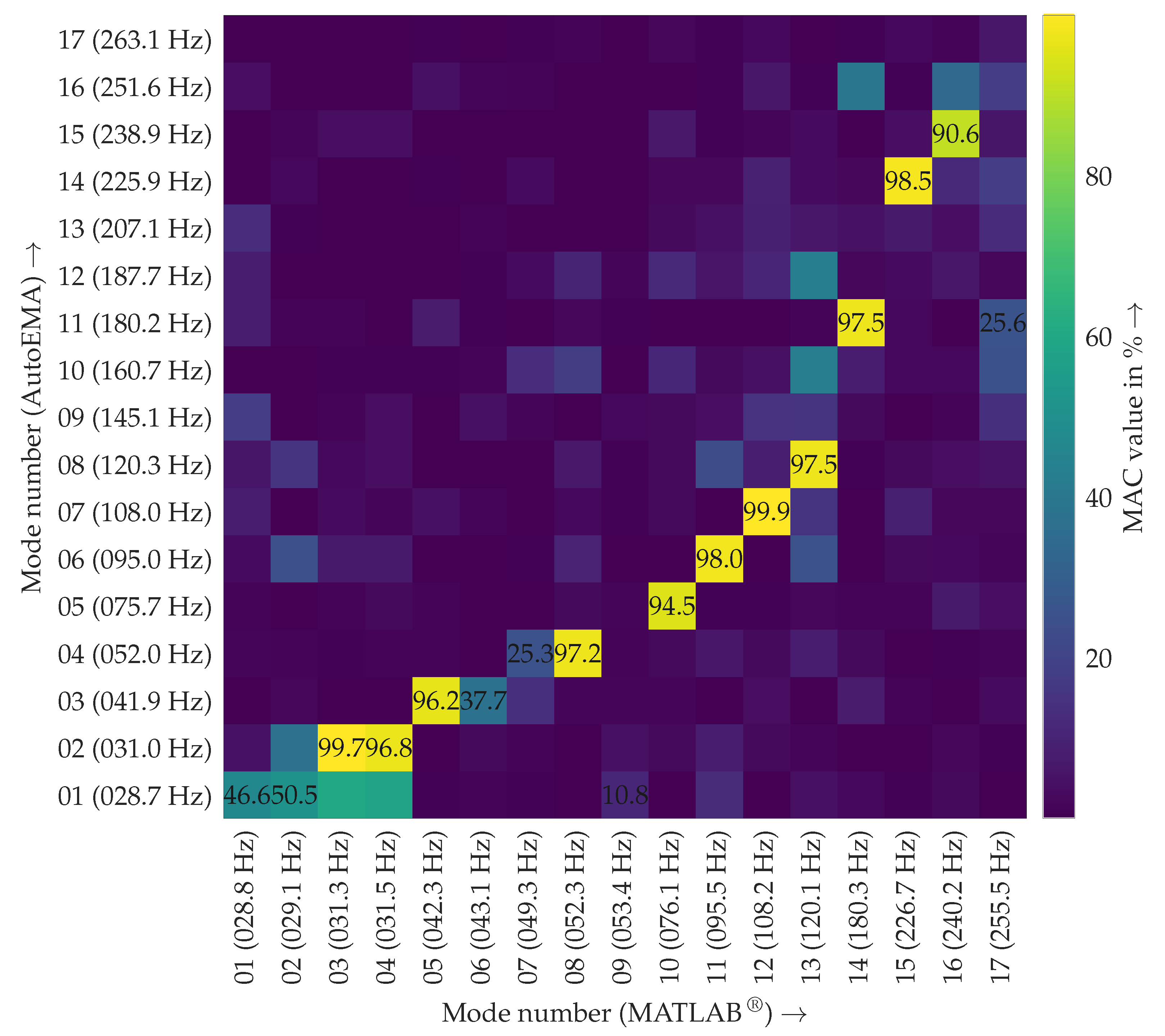
Figure 8 shows the correlation between the mode shapes found by MATLAB^® and the proposed approach for the frequency range up to 300 $\mathrm{Hz}$, which was determined by the MAC. It can be seen that most modes were found by both methods, indicated by MAC values higher than 80%. However, some modes were only found by the AutoEMA method but not by the MATLAB^® function, and vice versa. Given that, as will be shown below, the match between the modal models and the input data was very high in both cases, this result indicates modes that were either not well observed or highly damped.

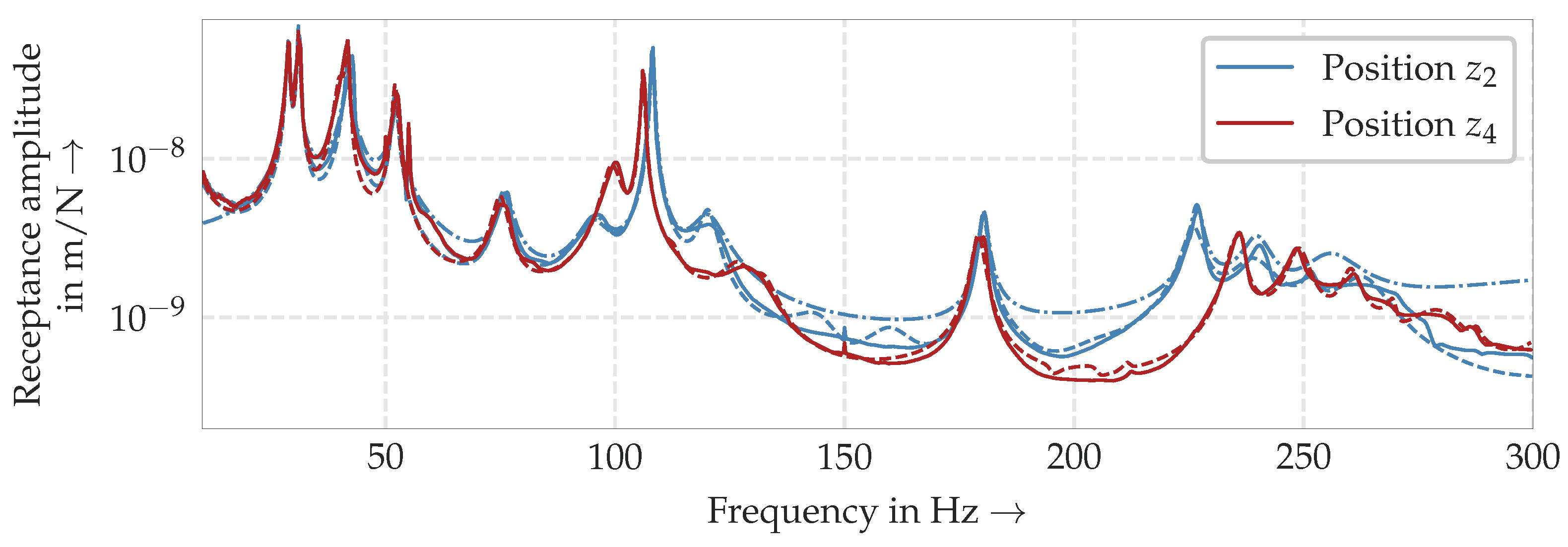
Figure 9 qualitatively illustrates the resulting match between the mean input FRFs and the reconstructed mean FRFs from the modal model for two WPT positions. It can be seen that there is a very high level of concordance between the input and fitted data for both positions for the AutoEMA approach, thus highlighting the validity of the model. However, there were higher deviations for the MATLAB^® approach at position $z_2$, especially in the high frequency region. This outcome was also confirmed by the mean FRAC values of $88.7$% for the AutoEMA FRF at position z${}_2$ and $64.8$% for the MATLAB^® FRF, respectively. In general, even FRAC values of 70% are considered to be a good match [22].

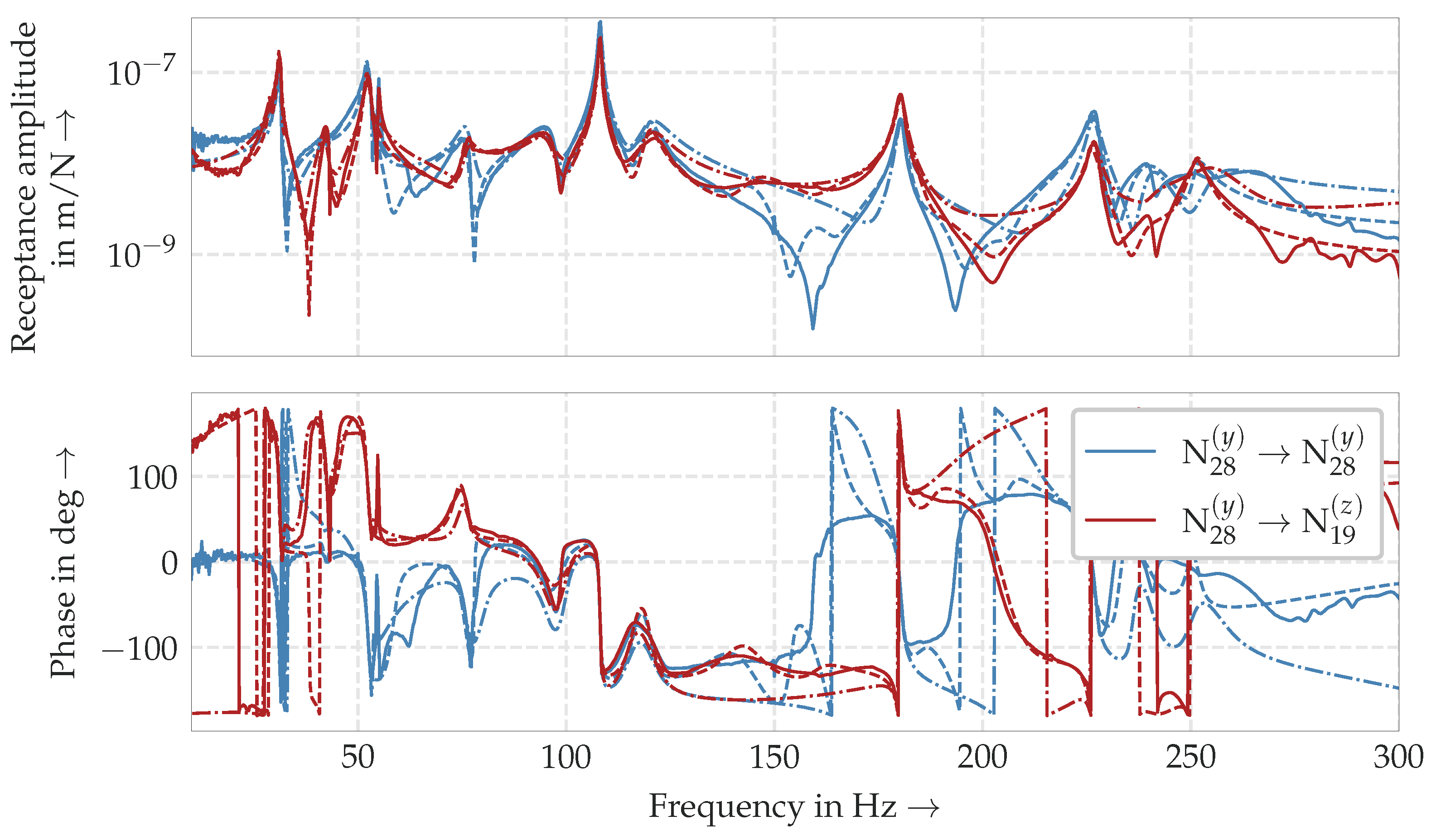
The same conclusion can be drawn by looking at the individual FRFs in Figure 10. It can be seen that, for both approaches, the direct driving point FRF from a force at node $N_{28}$ in the y-direction to the measured displacement at the same node in the same coordinate direction and the FRF from a force at node $N_{28}$ in the y-direction to the measured deflection at one of the edges of the machine tool (node $N_{19}$) in z-direction were approximated very well by the modal models. Regarding the AutoEMA approach, the same was also true for other FRFs, which is shown in

Table 7. FRAC value statistics for FRFs measured for WPT position z${}_2$ for the machine tool use case.

	Minimum	10% Percentile	Mean	Median	Maximum
AutoEMA	61.0%	82.0%	88.6%	90.1%	94.7%
MATLAB®	0.1%	18.9%	64.8%	73.3%	99.7%

: Only for 10% of the measured FRFs at all WPT positions, the modal model leads to a fitted FRF with, measured by the FRAC value, less than $82.6$% concordance. However, the MATLAB^® approach on average approximates the input FRFs only with a match of $64.8$% and one-tenth of them even worse than with $18.9$% concordance.

Table 8. Comparison of eigenfrequencies $f_i^e$ found by MATLAB^® and AutoEMA for WPT position z${}_2$; "-" indicates that no matching mode with a MAC value of at least 80% was found.

	${\mathit{f}}_1^{\mathit{e}}$	${\mathit{f}}_2^{\mathit{e}}$	${\mathit{f}}_3^{\mathit{e}}$	${\mathit{f}}_4^{\mathit{e}}$	${\mathit{f}}_5^{\mathit{e}}$	${\mathit{f}}_6^{\mathit{e}}$	${\mathit{f}}_7^{\mathit{e}}$	${\mathit{f}}_8^{\mathit{e}}$
AutoEMA	28.8 $\mathrm{Hz}$	31.0 $\mathrm{Hz}$	41.8 $\mathrm{Hz}$	52.1 $\mathrm{Hz}$	75.7 $\mathrm{Hz}$	95.0 $\mathrm{Hz}$	108.1 $\mathrm{Hz}$	120.0 $\mathrm{Hz}$
MATLAB®	-	31.3 $\mathrm{Hz}$	42.3 $\mathrm{Hz}$	52.3 $\mathrm{Hz}$	76.1 $\mathrm{Hz}$	95.5 $\mathrm{Hz}$	108.2 $\mathrm{Hz}$	120.1 $\mathrm{Hz}$
$\mathrm{N}\mathrm{F}{\mathrm{D}}_{AE-ML}$	-	1.1%	1.2%	0.3%	0.4%	0.6%	0.1%	0.1%

shows a comparison of eigenfrequencies estimated by the MATLAB^® and the AutoEMA approach for the machine tool data use case. It can be seen that both approaches estimate very similar eigenfrequencies with a maximum NFD (see Equation (6)) of only $1.2$%. This holds especially true considering that even a mean relative eigenfrequency difference of $3.3$% is sufficient for many applications [23]. However, the MATLAB^® approach seemed to generally estimate higher modal damping ratios with NDDs up to $213.7$%, as can be seen in

Table 9. Comparison of modal damping ratios ${\xi }_i$ found by MATLAB^® and AutoEMA for WPT position z${}_2$; "-" indicates that no matching mode with a MAC value of at least 80% was found.

	${\mathit{\xi }}_1$	${\mathit{\xi }}_2$	${\mathit{\xi }}_3$	${\mathit{\xi }}_4$	${\mathit{\xi }}_5$	${\mathit{\xi }}_6$	${\mathit{\xi }}_7$	${\mathit{\xi }}_8$
AutoEMA	1.05%	0.88%	1.67%	1.04%	1.98%	3.82%	0.29%	1.50%
MATLAB®	-	2.78%	2.75%	1.68%	2.22%	3.20%	0.28%	3.02%
$\mathrm{N}\mathrm{D}{\mathrm{D}}_{AE-ML}$	-	213.7%	64.8%	62.2%	12.2%	19.2%	5.8%	101.0%

.

Table 10. Identified first eight eigenfrequencies $f_i^e$ for the WPT position $z_2$ with the lowest number of found modes and the equivalent modes’ eigenfrequencies at the other positions; “-” indicates that no matching mode with a MAC value of at least 80% was found.

	${\mathit{f}}_1^{\mathit{e}}$	${\mathit{f}}_2^{\mathit{e}}$	${\mathit{f}}_3^{\mathit{e}}$	${\mathit{f}}_4^{\mathit{e}}$	${\mathit{f}}_5^{\mathit{e}}$	${\mathit{f}}_6^{\mathit{e}}$	${\mathit{f}}_7^{\mathit{e}}$	${\mathit{f}}_8^{\mathit{e}}$
$z_1$	28.7 $\mathrm{Hz}$	31.0 $\mathrm{Hz}$	-	52.0 $\mathrm{Hz}$	76.1 $\mathrm{Hz}$	91.9 $\mathrm{Hz}$	109.1 $\mathrm{Hz}$	117.3 $\mathrm{Hz}$
$z_2$	28.8 $\mathrm{Hz}$	31.0 $\mathrm{Hz}$	41.8 $\mathrm{Hz}$	52.1 $\mathrm{Hz}$	75.7 $\mathrm{Hz}$	95.0 $\mathrm{Hz}$	108.1 $\mathrm{Hz}$	120.0 $\mathrm{Hz}$
$z_3$	28.7 $\mathrm{Hz}$	31.0 $\mathrm{Hz}$	41.4 $\mathrm{Hz}$	52.1 $\mathrm{Hz}$	75.2 $\mathrm{Hz}$	97.9 $\mathrm{Hz}$	107.0 $\mathrm{Hz}$	122.4 $\mathrm{Hz}$
$z_4$	-	31.0 $\mathrm{Hz}$	-	52.1 $\mathrm{Hz}$	75.0 $\mathrm{Hz}$	-	106.1 $\mathrm{Hz}$	127.3 $\mathrm{Hz}$

and

Table 11. Identified first eight modal damping ratios ${\xi }_i$ for the WPT position $z_2$ with the lowest number of found modes and the equivalent modes’ damping ratios at the other positions; “-” indicates that no matching mode with a MAC value of at least 80% was found.

	${\mathit{\xi }}_1$	${\mathit{\xi }}_2$	${\mathit{\xi }}_3$	${\mathit{\xi }}_4$	${\mathit{\xi }}_5$	${\mathit{\xi }}_6$	${\mathit{\xi }}_7$	${\mathit{\xi }}_8$
$z_1$	1.04%	0.85%	-	1.18%	1.93%	3.59%	0.33%	1.54%
$z_2$	1.05%	0.88%	1.67%	1.04%	1.98%	3.82%	0.29%	1.50%
$z_3$	1.12%	0.86%	2.34%	1.03%	1.98%	2.27%	0.29%	2.66%
$z_4$	-	0.96%	-	1.01%	2.16%	-	0.32%	2.93%

show the first eight identified eigenfrequencies and modal damping ratios using the AutoEMA method for WPT position z${}_2$, which is the one with the lowest number of identified eigenmodes (26 modes up to 300 $\mathrm{Hz}$). Similar modes at the other positions were found using the MAC [24], and their eigenfrequencies and damping ratios are also listed. It can be seen that the modes 1 to 4 exhibited only a low level of dependency on the WPT position, whereas the eigenfrequency and modal damping ratios of modes 5 to 8 changed from position z${}_1$ to position z${}_4$. This result can also be seen in the comparison of the mean measured and fitted FRFs in Figure 9.

4. Conclusions and Outlook

This paper presented an approach for automatically estimating the modal parameters of a system based on input measurements. In contrast to the state-of-the-art, no user input is needed for evaluating the stabilization diagram, nor is the solution space restricted by fixed rules derived from the input data set. Instead, a Bayesian optimization process ensures that modal parameters are found, thus leading to the model best representing the original input data. The proposed AutoEMA approach was first theoretically derived in Section 2, and was validated using simulated input data from an MDOF oscillator. The approach was benchmarked against ground truth reference values and the MATLAB^® modalfit function in this context. Finally, the proposed approach was also applied to EMA data from a machine tool test bench. It was found that the AutoEMA approach led to modal parameters which effectively represent the original input data for different machine tool axis positions, thereby outperforming the MATLAB^® method in both accuracy and calculation time.

Although this approach has already been successfully tested on two very different data sets (see Section 3), future research will further validate the proposed approach. Data from domains other than machine tools will be used for this purpose. Special attention will be paid to very closely spaced modes, symmetrical modes, and heavily coupled modes. Currently, the presented approach is limited to EMA with FRFs as input data. It will be examined in the future if and how it can be extended to work with OMA and, for example, power spectral densities as input data. Moreover, the AutoEMA method now offers a means of reliably extracting modal parameters in a computationally efficient manner. It will be researched how this information can be used best in parameter identification of machine tool models.

References

1. Lau, J.; Lanslots, J.; Peeters, B.; van der Auweraer, H. Automatic Modal Analysis—Myth or Reality? In Proceedings of the 25th International Modal Analysis Conference, Orlando, FL, USA, 19–22 February 2007.
2. Verboven, P. Frequency-Domain System Identification for Modal Analysis. Ph.D. Thesis, Vrije Universiteit Brussel, Brussels, Belgium, 2019. [Google Scholar]
3. Ellinger, J.; Zaeh, M.F. Automated Identification of Linear Machine Tool Model Parameters Using Global Sensitivity Analysis. Machines 2022, 10, 535. [Google Scholar] [CrossRef]
4. Reynders, E. System Identification Methods for (Operational) Modal Analysis: Review and Comparison. Arch. Comput. Methods Eng. 2012, 19, 51–124. [Google Scholar] [CrossRef]
5. Ewins, D. Modal Testing: Theory, Practice and Application, 2nd ed.; Mechanical Engineering Research Studies; Research Studies Press: Baldock, UK, 2000; Volume 10. [Google Scholar]
6. Altintas, Y. Manufacturing Automation: Metal Cutting Mechanics, Machine Tool Vibrations, and CNC Design; Cambridge University Press: Cambridge, UK, 2012. [Google Scholar]
7. Ozdemir, A.; Gumussoy, S. Transfer Function Estimation in System Identification Toolbox via Vector Fitting. IFAC-PapersOnLine 2017, 50, 6232–6237. [Google Scholar] [CrossRef]
8. Vold, H.; Kundrat, J.; Rocklin, T.; Russell, R. A Multi-Input Modal Estimation Algorithm for Mini-Computers; SAE Technical Paper Series; SAE International: Warrendale, PA, USA, 1982. [Google Scholar] [CrossRef]
9. Peeters, B.; van der Auweraer, H.; Guillaume, P.; Leuridan, J. The PolyMAX Frequency-Domain Method: A New Standard for Modal Parameter Estimation? Shock Vib. 2004, 11, 395–409. [Google Scholar] [CrossRef]
10. van Overschee, P.; de Moor, B. Subspace Identification for Linear Systems; Springer: Boston, MA, USA, 1996. [Google Scholar] [CrossRef]
11. Scionti, M.; Lanslots, J. Stabilisation Diagrams: Pole Identification Using Fuzzy Clustering Techniques. Adv. Eng. Softw. 2005, 36, 768–779. [Google Scholar] [CrossRef]
12. Reynders, E.; Houbrechts, J.; de Roeck, G. Fully Automated (Operational) Modal Analysis. Mech. Syst. Signal Process. 2012, 29, 228–250. [Google Scholar] [CrossRef]
13. Scionti, M.; Lanslots, J.; Goethals, I.; Vecchio, A.; van der Auweraer, H.; Peeters, B.; de Moor, B. Tools to Improve Detection of Structural Changes from In-Flight Flutter Data. In Proceedings of the 8th International Conference on Recent Advances in Structural Dynamics, Southampton, UK, 14–16 July 2003. [Google Scholar]
14. van der Auweraer, H.; Peeters, B. Discriminating Physical Poles from Mathematical Poles in High Order Systems: Use and Automation of the Stabilization Diagram. In Proceedings of the 21st IEEE Instrumentation and Measurement Technology Conference (IEEE Cat. No.04CH37510), Como, Italy, 18–20 May 2004; pp. 2193–2198. [Google Scholar] [CrossRef]
15. Neu, E.; Janser, F.; Khatibi, A.; Orifici, C. Fully Automated Operational Modal Analysis Using Multi-Stage Clustering. Mech. Syst. Signal Process. 2017, 84, 308–323. [Google Scholar] [CrossRef]
16. Mugnaini, V.; Zanotti, L.; Civera, M. A Machine Learning Approach for Automatic Operational Modal Analysis. Mech. Syst. Signal Process. 2022, 170, 108813. [Google Scholar] [CrossRef]
17. Zaletelj, K.; Bregar, T.; Gorjup, D.; Slavič, J. pyEMA. 2020. Available online: https://zenodo.org/record/4016671#.Y7vYsBVBzIU (accessed on 26 December 2022).
18. Garnett, R. Bayesian Optimization; Cambridge University Press: Cambridge, UK, 2022. [Google Scholar]
19. Heylen, W.; Lammens, S. FRAC: A Consistent Way of Comparing Frequency Response Functions. In Identification in Engineering Systems; Friswell, M.I., Mottershead, J., Eds.; University of Wales: Swansea, UK, 1996; pp. 48–57. [Google Scholar]
20. Allemang, R. The Modal Assurance Criterion – Twenty Years of Use and Abuse. J. Sound Vib. 2003, 37, 14–23. [Google Scholar]
21. Imamovic, N. Validation of Large Structural Dynamics Models Using Modal Test Data. Ph.D. Thesis, Imperial College of Science, Technology & Medicine, London, UK, 1998. [Google Scholar]
22. Semm, T.; Sellemond, M.; Rebelein, C.; Zaeh, M.F. Efficient Dynamic Parameter Identification Framework for Machine Tools. J. Manuf. Sci. Eng. 2020, 142, 081003. [Google Scholar] [CrossRef]
23. Hernandez-Vazquez, J.; Garitaonandia, I.; Fernandes, M.H.; Munoa, J.; Lacalle, L.N. A Consistent Procedure Using Response Surface Methodology to Identify Stiffness Properties of Connections in Machine Tools. Materials 2018, 11, 1220. [Google Scholar] [CrossRef] [PubMed] [Green Version]
24. Vacher, P.; Jacquier, B.; Bucharles, A. Extensions of the MAC Criterion to Complex Modes. In Proceedings of the 24th International Conference on Noise and Vibration Engineering, 2010, Proceedings of ISMA2010 Including USD2010, Leuven, Belgium, 20–22 September 2010; pp. 2713–2726. [Google Scholar]
Figure 1. Flowchart showing the AutoEMA method; the modal parameter estimation is based on a set of hyperparameters explained in Table 1. Their value is determined by a Bayesian optimization strategy such that the resulting model optimally replicates the original input data.
Applsci 13 00949 g001
Figure 2. Exemplarily FRF and potentially physical poles identified after applying the PolyMAX algorithm and criteria (a) to (d) (see Section 2.1) for the given hyperparameters k Δ f , k Δ D , k D m i n , and k D m a x .
Applsci 13 00949 g002
Figure 3. Identified modes by agglomerative clustering with a maximum frequency distance d m a x of poles within a cluster; different clusters, that is, distinct modes, are indicated by different colors. The finally selected poles are marked with a cross.
Applsci 13 00949 g003
Figure 4. Schematic illustration of an MDOF system used for generating synthetic measurement data in Section 3.1.
Applsci 13 00949 g004
Figure 5. Comparison of the receptance amplitude and the phase between the input (solid) and the fitted FRF (AutoEMA: dashed, MATLAB®: dash-dotted) from the modal model from a force f 1 to the displacement x 1 of the first mass; normal (Gaussian) noise was added to the (synthetic) displacement data to simulate noisy real-world measurements.
Applsci 13 00949 g005
Figure 6. Comparison of the found mode shapes using the MAC; here, the mode shapes from solving the damped eigenvalue problem resulting from the MDOF oscillator in Section 3.1 were used as ground truth, (a) MATLAB® modalfit, (b) AutoEMA.
Applsci 13 00949 g006
Figure 7. Rendering of the considered machine tool, the measurement positions z 1 to z 4 , and the measured nodes; the WPT is depicted in position z 3 and a description of the node points can be found in Table 5.
Applsci 13 00949 g007
Figure 8. Correlation between the modes up to 300 Hz found by the AutoEMA approach and MATLAB®modalfit determined by the MAC for the WPT position z 2 .
Applsci 13 00949 g008
Figure 9. Comparison of the mean receptance amplitude of the original input FRFs (solid) with the fitted FRFs from the modal model (MATLAB®: dash-dotted, AutoEMA: dashed); the comparison is shown for the WPT positions having the lowest number of found modes z 2 and the one at the greatest distance, that is, position z 4 . Due to the high calculation times, MATLAB® results are only available for position z 2 .
Applsci 13 00949 g009
Figure 10. Comparison of the receptance amplitude and the phase between measured (solid) and fitted FRFs (MATLAB®: dash-dotted, AutoEMA: dashed) from the modal model for position z 2 ; N α 1 ( β 1 ) → N α 2 ( β 2 ) denotes the FRF between a force excitation at node N α 1 in coordinate direction β 1 and the measured displacement at node N α 2 in coordinate direction β 2 (see Table 5).
Applsci 13 00949 g010