1. Introduction
In large hub airports, aircraft stands can be categorized into two types, the near parking stand and the remote. The nearby positions are fully equipped with all kinds of support equipment, including the power supply, corridor bridges, refueling pipelines, water supply and drainage pipelines. Remote positions need to rely on ground support vehicles, including power supply vehicles, stepladder vehicles, ferries and refueller trucks. With the increase in flights at the airport, it is difficult to continuously improve the utilization rate of the nearby parking stands. More and more flights will be parked at the remote parking stands, which will gradually increase the demand for ground support vehicles. Meanwhile, due to the influence of weather, airspace control, passenger behavior and other factors, it is unavoidable that there are deviations between the actual arrival and departure times of flights and the planned times. At present, the basic information that ground support resource scheduling relies on is the estimated flight arrival and departure times and the information returned from the scene. The lag and one-sidedness of the information have a great impact on the decision making related to ground support resource scheduling. Therefore, the punctuality of flights is the main factor affecting the utilization efficiency of ground support resources. Under the uncertainty of flight arrival and departure times, the rational allocation and effective utilization of ground support resources become more important.
The flight ground support process is a service structure that is temporal and mutually exclusive. Knster et al. [
1] defined the ground support process as a resource-constrained project scheduling problem (RCPSP) and proposed an evolutionary algorithm to solve it. Limited by computational efficiency, vehicle route planning with time windows (VRPTW) has progressively become a major approach to studying the problem of scheduling ground support resources. Concerning the centralized ground support resource scheduling problem, Padrón et al. [
2] decomposed the original problem. A heuristic was designed to solve each subproblem. In some studies, the flight transit process was defined as a whole. The specific scheduling of the various types of supported services of the transit process was not considered, including in [
3,
4]. The results of both studies showed that there are two factors affecting the punctuality of flight departures. They are the length of flight transit time and the efficiency of ground support services. To solve the airside scheduling problem at airports, Clausen [
5] and Weiszer et al. [
6] conducted research in two distinct directions. The former proposed a multi-level rolling scheduling framework for the support resource scheduling problem under flight arrival uncertainty. The upper layer was a dynamic demand model, which forecasts the demand under the influence of stochastic factors. The middle layer was a resource planning model. The lower layer was a task scheduling model. The latter started from a horizontal perspective. Researchers proposed a multi-objective integrated optimization problem by considering the lack of information sharing at all stages. They solved multi-module problems including runway scheduling, flight taxiing and ground resource scheduling through a joint scheduling method.
The flight transit process is also complex. In actual operation and management, different types of resources are divided into different business offices. Different support resources have a high degree of independence in management. Therefore, most of the studies on the scheduling problem of ground support resources focus on the co-scheduling of a small number of types of resources [
7,
8] and single-type resource scheduling [
9,
10]. The combination of resource types in multi-resource co-scheduling problems has a different impact on the research methodology. Zhu et al. [
11] investigated the problem of cooperative scheduling of the ferry and refueller. Due to the airport support manual, the process of passenger loading and unloading is not performed at the same time as refueling. Ip et al. [
12] proposed a multi-agent-based decision support model to minimize the vehicle allocation cost in the multi-resource cooperative scheduling problem of water trucks, cleaning trucks and tractors. Common single-type resource scheduling problems include tractor [
13,
14], ferry, de-icing vehicle and taxiway scheduling. Du et al. [
13] constructed a mixed-integer programming model based on the vehicle routing problem (VRP) as the core with the minimum operation cost as the optimization objective. Then, they proposed a column generation heuristic solution method. In terms of the optimization objective, Du et al. [
14] comprehensively considered the cost impacts of various aspects such as tractor configuration cost, maintenance cost and secondary sales. They aimed to obtain a fleet composition with the lowest cost. The fleet composition had a large impact on the operating cost. Bao et al. [
15] considered the impact of electric equipment on the previous fuel-only fleet composition model. They synthesized the time cost, energy cost and scheduling cost to provide a reference for the introduction of electric equipment in airports. The airport special vehicle traveling road network is a complex multi-loop structure with multiple paths between any two points. Ding et al. [
16] emphasized that the basis of the rationality of ferry scheduling lies in the transfer between nodes. For this reason, the transfer time between nodes was mined through graph theory. The Floyd algorithm was used to obtain the shortest paths and times of all origin–destination (OD) points. In the process of transferring, in addition to the distance and time, other optimization components need to be considered. In [
17], an active path framework was proposed for the resource movement problem, which can support the selection of multi-objective paths. In the static problem, an enumeration-based algorithm was designed to provide optimal or suboptimal solutions quickly. Li et al. [
18] constructed a quadratic planning model with VRPTW as the core to obtain a scheduling scheme for the minimum number of ferry usage.
Uncertainty is inherent in the ground support resource scheduling problem [
19]. A flight is defined as on-time if its actual arrival and departure time deviates less than 15 min from the estimated arrival and departure time. This deviation time cannot be ignored in the problem of actual ground support resources. Research for uncertainty problems can be classified into the following methods: delayed decision making [
5,
20], robust optimization [
21,
22,
23] and stochastic planning [
19,
24,
25,
26]. The basic principle of delayed decision making is to make the original fuzzy uncertainty certain by postponing the decision as much as possible. In [
20], considering the impact of uncertainty in flight arrival and departure times on tractor scheduling, accessing the A-CDM system was proposed, which can obtain basic data with higher reliability. The A-CDM data reliability was reflected in the dynamic prediction, which made the support resource scheduling not only dependent on the scene feedback or flight schedule. In terms of robustness optimization, a more robust scheduling scheme was generated based on existing resources. Wang et al. [
22] increased the stability of task sequences for each guaranteed resource execution by maximizing the buffer time between support resource execution services. This method could improve the robustness of the overall scheduling scheme. However, it often did not intuitively show the degree of resource surpluses and deficits. It was necessary to react to the reasonableness of the current resource allocation through simulation or actual execution results. Like robust optimization, stochastic planning makes decisions under the inevitable presence of uncertainty. Multi-scenario is a common approach. Yang et al. [
24] described the original uncertainty problem with many deterministic scenarios through multi-scenarios for the flight taxi scheduling problem. The biggest difficulty of this method is the probability of each deterministic scenario. Unlike the multi-scenario approach, the sample average approximation (SAA) method assumes equal probability for each sample. Since the SAA method does not need to depend on the probability of each scenario, it is easy to implement and is increasingly recognized by researchers. Due to its equal probability nature, the sample size is a very important parameter. With too small a sample size, the results are highly episodic, and with too large a sample size, the impact of the problem size on the computational efficiency increases exponentially. Both [
19,
20] used chance constraints to describe stochastic problems while designing some efficient heuristics.
This paper focuses on the ferry scheduling problem considering the in-place time requirement under the uncertainty of flight arrival and departure times. The ferry is an important means of transportation for passengers to transfer between the remote parking stand and the terminal. As each flight carries a different number of passengers, the number of ferry demands is also different. The object of the ferry service is passengers, and safety and timeliness are important indicators of the airport’s original airfield security services. Therefore, most airports require ferries to arrive at the designated position a certain time in advance to wait when the flight ferry service time arrives. According to Civil Aviation Authority (CAA) regulations, when multiple ferries are required for a flight, the first ferry needs to be in place a certain amount of time in advance. The subsequent ferries need to be in place within a certain amount of time of the departure of the previous ferry with passengers. Therefore, the problem of scheduling multiple ferries on the same flight is essentially a dynamic programming problem. In this paper, according to the characteristics of the ferry scheduling problem, the dynamic programming model is constructed, and the minimum number of ferry cars is used as the optimization objective. Considering the uncertainty of flight arrival and departure time, the uncertainty is described by opportunity constraints, the model is transformed into a stochastic model, and a genetic algorithm (GA) is designed to solve the probabilistic model.
The remaining contents of this paper are organized as follows. In
Section 2, the ferry scheduling problem is analyzed in detail, and the dynamic programming scheduling model of the ferry is constructed in the static case considering the in-place time requirement. In
Section 3, the impact of flight arrival and departure time on ferry scheduling is considered, and the chance constraints are used to describe the uncertainty of the problem, which transforms the original model into a stochastic dynamic programming model. To solve the stochastic dynamic programming model, the stochastic model is transformed into a deterministic model, and a genetic algorithm is designed to solve it. In
Section 4, the data from an international airport in South China is used as the experimental case of this paper. The summary section is presented in
Section 5.
2. Problem Description and Model Construction
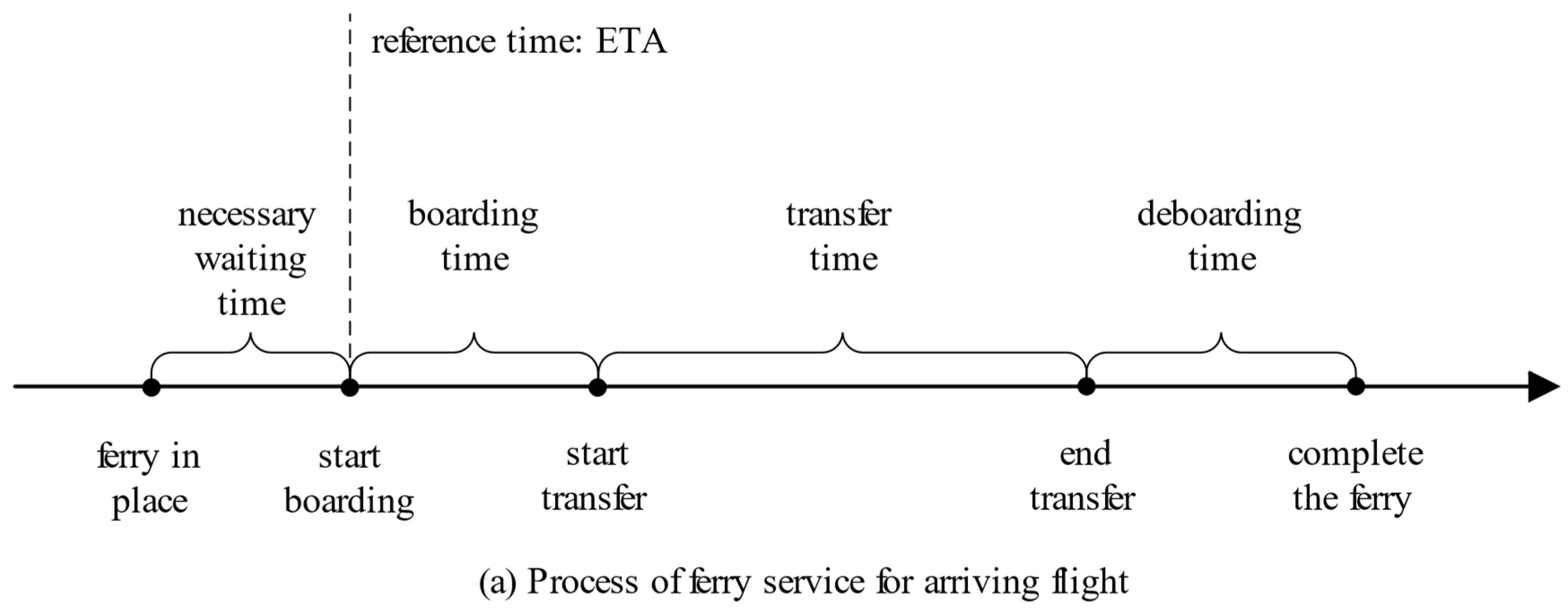
The flight transit process can be divided into two parts, inbound and outbound. Both inbound and outbound flights at remote locations require ferry service. The inbound ferry service relies on the base time of the flight’s estimated time of arrival (ETA). The outbound ferry service relies on the base time of the flight’s estimated time of departure (ETD). With the flight inbound and outbound times determined, the start time of the first ferry service for the flight can be determined as well as the in-place time. A complete ferry service consists of four components: the necessary in-place time, the passenger boarding time, the transfer time and the passenger deboarding time. For the inbound ferry service, the base time is ETA. The relative relationship between the above components of the inbound ferry service is shown in
Figure 1a. The first ferry is in place well in advance of the flight arrival, and passengers are transferred from the airplane to the ferry when the inbound ferry service arrives. Passenger boarding ends when the last passenger on board is reached or when the number of passengers on board reaches the capacity limit. At the same time, the ferry transfers passengers from the aircraft to the terminal, and the passengers get off. This is the complete service process performed for one ferry. The base time of the departure ferry is ETD. Through the ferry service standard of each airline company, it can be known how far in advance the ferry service of each flight has to start, thereby determining the start time of the outbound ferry, as shown in
Figure 1b. When the ferry service requires multiple ferries, the first ferry’s arrival time and start time are based on the arrival time of the ferry service. The arrival and service time of the non-first ferry is determined by the designation of the previous ferry.
The ferry scheduling problem considering the in-place time can be described as follows.
During a decision cycle, there are flights parked at remote parking stands that need to perform an inbound or outbound process. Each flight has a ferry service, and all ferry services in the decision cycle are defined as the set . Let be the index of the set of ferry services, and there are and . Due to the large difference in the number of passengers carried by different flights, the number of ferries required by different ferry services is not equal. Define as the index of a sub-service of ferry service . Then, for service , there is . The set of ferry cars is defined as such that . When the decision variable takes the value of 1, it indicates that the th sub-service of ferry service is executed by ferry car and otherwise is 0. Correspondingly, the decision variable denotes the time at which ferry is in place to execute the th sub-service of ferry service . The decision variable denotes the start time of the th sub-service of the ferry service . The complete ferry service contains four components: the necessary in-place time, the passenger boarding time , the transfer time between the airside and the terminal and the passenger deboarding time . For the inbound ferry service, the initial position of the ferry is the stop. The target position is the terminal. And is used as the necessary transfer time between the aircraft position and the terminal. Setting as a ferry service different from , is used to denote the necessary transfer time between different ferry services. Since the path of the ferry transferring between any two points is determined, there is . The other parameters and decision variables of the model are represented as follows.
The airport vehicle road network is a complex multi-loop structure. To minimize the impact of the ferries on the taxi path of the aircraft, they usually follow fixed routes. In the problem studied in this paper, the ferry travel distance is not considered as an optimization objective. In the case of considering the ferry in-place time difference pairs, the most infrequent use of the ferry is used as the only optimization objective, as shown in Equation (1). Due to the uncertain arrival time of the ferry service, the in-place time of the non-first ferry can slide. In
Figure 2, the horizontal axis represents time, and the vertical axis represents the required number of ferries. The rectangular square represents the ferry service. The dashed lines at both ends of the rectangle indicate the possible sliding range. By coordinating the arrival time of ferry services for different flights, the number of ferries used during the decision-making cycle is minimized. At time point
, coordinating the start time of service
and
can reduce the instantaneous demand for ferries.
where
is used as a statistical decision variable for whether the ferry
is enabled or not in the decision cycle, as shown in Equation (2).
In Equation (2), when ferry
does not perform any of the sub-services
of ferry service
, the number of configured ferries is in surplus in that decision cycle.
The same ferry service
contains several sub-services
, and each sub-service requires one ferry. From the uniqueness point of view, any ferry sub-service can only be executed by one ferry, as shown in Equation (3).
In Equations (4)–(7), Equation (7) serves as a common value range constraint for the variables in Equations (4)–(6). For any two unequal ferrying services, the decision variable takes the value of 1 when the same resource executes service before service . It is also necessary to satisfy the time for service to start ferrying until all of the work of service has been completed and still leave enough transfer time to service .
Among the studies of the ferry scheduling problem, there are several common treatments to simplify the description of the problem. In the first type, it is assumed that each flight needs at most one ferry to provide service. To adapt to the actual problem,
virtual flights are introduced when the number of flights needing ferries is
uj > 1. It is required that the inbound and outbound times of the introduced virtual flights are the same as shown in
Figure 3a [
27]. The problem with this method is that the start and end times of the split ferry sub-service and the original ferry service are identical. The second type is based on the time window of the earliest start of the ferry service
and the latest start of the ferry service
combined with the number of ferries needed for the flight to equalize the division [
10]. The earliest start time and the latest start time defined in this method are both before the arrival time of the ferry service, as shown in
Figure 3b.
Existing splitting methods for flights requiring multiple ferries mainly simplify the problem by ignoring interrelationships between multiple ferries. These treatments are not conducive to the utilization of ferry resources. According to the CAA, when the flight ferry service requires multiple ferry vehicles to provide service, the first ferry vehicle
, and the in-place time
needs to be in front of the arrival time
of the flight ferry service and at least
in advance, as shown in
Figure 3c. The non-first ferry
, and the arrival time
needs to arrive within the maximum time interval
after the previous ferry leaves. Therefore, the requirements for the arrival time of each sub-service of the ferry are as in Equation (8).
Correspondingly, Equation (9) represents the requirement of the start time of each sub-service of the ferry. takes the value of 1, which means that ferry executes the sub-service of ferry service . When its in-place time arrives before the departure of the previous sub-service ferry, its start time is equal to the time of the departure of the service ferry; otherwise, it is the actual arrival time of the ferry while satisfying the constraints of Equation (8).
3. Problem Transformation and Model Solving
In the previous section, the ferry scheduling problem considering the difference in in-place time under the determination of the arrival time of ferry service is analyzed. A nonlinear dynamic programming model with the number of ferry usage as the optimization objective is established. In the decision cycle, the estimated arrival and departure times of flights deviate too much from the actual times. The effect of this deviation on the scheduling scheme cannot be ignored. Therefore, the ferry scheduling problem is a ferry dynamic scheduling problem under stochastic conditions.
3.1. Model Transformation
Chance-constrained programming is an important branch of stochastic programming, which was jointly proposed by A. Chames and W.W. Cooper in 1959 [
28]. In stochastic scheduling problems, a comprehensive response to uncertainty can lead to excessive resource demand due to stochastic factors. In chance-constrained programming, a balance is obtained between the penalty cost from not satisfying the constraint and the resource allocation cost by allowing a certain degree of non-satisfaction with the constraint. Chance constraints are commonly used to obtain a scheduling plan that satisfies the confidence level of constraint satisfaction by presetting the level of confidence
at which the constraint is satisfied. The deviation between the estimated arrival and departure times of flights and the actual times is unavoidable [
19]. For example, the start time of the ferry service
is not certain at the time of decision making. For this reason, the random variable
is redefined to denote the arrival time of ferry service
.
is used to denote the probability of event
. The mathematical description is presented in
Section 2, and Equation (8) needs to be transformed into Equation (10).
In Equation (10), the start time of the sub-service
of ferry service
is not fully known. To ensure that ferry
can satisfy the arrival before the advance time
with different confidence levels, the chance constraints are used to describe the requirements of the ferry’s in-place time. When
, the ferry
in-place time for the sub-service
of
needs to fully satisfy the in-place time requirement of ferry service
with different arrival times. The directly defined random variable is
, and it is easy to know from the perspective of problem characterization that the range of values of
is affected by
. Therefore, all constraints related to service arrival time in
Section 2 can be understood as constraints with random variables. Equations (4) and (9), when considering random variables, are rewritten as follows:
In the original static problem, a random variable
is introduced. Equations (4), (8) and (9) associated with the random variable are transformed into chance constraints (10), (11) and (12), respectively. Due to the difficulty in describing the probability of the arrival time deviation of the ferry service, the model proposed in the above statement cannot be solved directly. Therefore, a SAA method is proposed to describe the above chance constraints. For the random variable
, set
such that
, where
are
independent and identically distributed samples of
. Introducing the indicator variable
,
takes the value 0 when
and otherwise is 1. Correspondingly,
is a sample of
when
, and the indicator variable
takes the value 0 and otherwise is 1. Thus, Equation (10) is transformed into Equations (13) and (14).
For Equation (11), when
, the indicator variable
takes the value 0 and otherwise is 1. Thus, Equation (11) is transformed into Equations (15) and (16).
For Equation (12), the indicator variables
and
are introduced. When
, the value of
is 0, and
can take −1 or 0. When
, the value of
is 0, and
can take −1 or 0. Therefore, Equation (12) can be transformed into Equations (17)–(19).
3.2. Genetic Algorithm Design
The ferry scheduling under the uncertainty of the arrival time of the ferry service considering the difference in in-place time is a complex problem. A SAA dynamic programming model is constructed with the minimum number of ferry usage as the optimization objective. To solve the model, a GA method based on Monte Carlo random sampling is designed, where represents the current number of samples and represents the size of the sample set. and represent the current iteration number and the maximum iteration number, respectively.
The detailed steps of GA are as follows.
Step 1: chromosome encoding and population initialization.
The ferry scheduling scheme contains service chains of multiple ferries. To easily transform the service chains into gene segments of chromosomes, a positive integer order encoding is used to denote all ferry sub-services to be assigned with . Each ferry service has sub-services, each of which corresponds to a different gene, and different gene orders represent different scheduling schemes. The initialization process of the population is to generate many chromosomes with randomly arranged genes.
Step 2: chromosome decoding and fitness evaluation.
Chromosome decoding is the process of transforming a chromosome into a scheduling solution. For example, there are 10 ferry sub-services to be assigned, and one randomly generated chromosome is . Assume that all ferries have the same state, that the airport has a parking lot denoted by 0 and that each ferry departs from the parking lot and eventually returns to it. All constraint-conflict-free sub-services such as are assigned to ferry 1 according to the gene order on chromosome A. By this analogy, we can obtain the ferry service chain as ; the service chain as ; and the service chain as . The combination of all service chains is the scheduling scheme. To evaluate the advantages and disadvantages of the scheduling scheme, the chromosome needs to be evaluated for fitness, which is the inverse of the number of service chains.
Step 3: selection operation.
The core idea of the selection operation is survival of the fittest. The purpose is to select the excellent individuals in the population and eliminate the inferior individuals. The fitness value of an individual is converted into the probability of the individual being selected. Commonly used selection operators are roulette selection, random traversal sampling, etc., the former of which is used in this paper.
Step 4: crossover operation.
The purpose of the crossover operation is to increase the diversity of the population and prevent premature convergence to a local optimum. The crossover operation will change the gene combinations of individuals to generate new individuals. Based on the positive integer arrangement coding method used in this paper, it is necessary to ensure that the chromosome genes are complete and not duplicated. If the conventional single-point crossover or multi-point crossover is used, it will generate non-compliant chromosomes with great probability. To address this problem, the crossover operator in this paper uses order crossover. The region between two randomly generated crossover points is defined as the crossover gene segment. After copying the crossover gene fragments, the remaining genes of the child chromosome are filled, and the complete child individual is obtained.
For example, crossover is performed on paternal chromosome and paternal chromosome .
Step 4.1: Duplicate crossover gene segments. Randomly select crossover points 4 and 8 and copy the crossover gene fragments from the paternal chromosomes A and B to the child chromosomes C and D, respectively, as shown in
Figure 4.
Step 4.2: Fill in the remaining genes of the child’s chromosome. The genes in the paternal chromosome A, except those already present in the child’s chromosome D, are filled into chromosome D in order, and similarly, the remaining genes in the child’s chromosome C are filled. This also results in two complete child individuals, as shown in
Figure 5.
Step 5: mutation operation.
The mutation operation generates new individuals by randomly changing their genes. It can increase the population diversity and improve the global search ability of the algorithm. When approaching the neighborhood of the optimal solution after the crossover operation, the convergence speed can be accelerated to some extent by the mutation operation.
The integrity and uniqueness of chromosome genes need to be guaranteed when mutation is performed. In this paper, we adopt the method of randomly selecting two or more different gene positions for the original chromosome to be interchanged to produce a new chromosome, as shown in
Figure 6.
Step 6: repeat the iteration.
4. Numerical Example Analysis
The actual data of an airport in South China is used as a numerical example. Information for 31 flights during the peak hour was obtained from the transportation control system, which contained 43 flight ferry services. The example information of the ferry service is shown in
Table 1. To better adapt to the data format of the model, “00:00:00” is defined as 0. We converted time into minutes as the minimum time particle. For example, we converted “10:00:00” to 600 and “12:27:00” to 747. According to the flight service standards provided by the airline company, we determined the required arrival time of the first ferry based on the ETD. A purely numerical code usually represents a stand number, such as “217” in
Table 1. A code with letters indicates the location of the terminal at the ferry, such as “W02” in
Table 1.
The deviation between the estimated flight time and the actual time cannot be ignored. Through analysis of a large amount of historical data, it was found that there are differences in the distribution of departure time deviation and arrival time deviation. For this reason, the departure time deviation and the arrival time deviation are described separately, as shown in
Figure 7a,b. The horizontal coordinate indicates the deviation between the estimated time and the actual time. When the value is negative, it indicates that the actual time of the flight is earlier than the estimated time. The deviation range of departure time is [−3, 16], and the deviation range of arrival time is [−9, 8]. From the process of the ferry, it is clear that the start time of the inbound ferry service depends on the actual arrival of the incoming flight. The start time of the outbound ferry service depends on the departure time of the flight. Consequently, it is a reasonable assumption to use the flight inbound and outbound time deviation distribution to describe the dynamics of the arrival time of the ferry service. Therefore, when the actual arrival and departure times of flights have not been determined, it is assumed that the arrival times of inbound and outbound ferry services obey the following discrete distributions.
4.1. Research on Algorithm Parameters
In
Section 3, a multi-parameter configurable GA was designed to effectively and quickly solve the model. This section studies the range of values for population size, iteration times and sample size.
Firstly, population size is an important indicator that affects the duration of a single iteration. In a single iteration, the larger the population size, the larger the search space of the algorithm. The more times the fitness of each individual is calculated, the lower the search efficiency. In contrast, the smaller the population size, the greater the number of iterations required. For the above case, assuming that the estimated arrival and departure time of the flight is strictly consistent with the actual time, the problem is the static scheduling problem of the ferry. By using precise algorithms to solve the final determination, without considering the uncertainty of flight arrival and departure time, the minimum number of ferries used is 10. In
Table 2, the changes in relevant indicators during the population size change from 10 to 100 are shown. For obtaining the optimal solution from the indicator of the maximum number of iterations, when the population size is small, the number of iterations needed to obtain the optimal solution is relatively similar and even limited by the set number of iterations. Similarly, there is a strong positive correlation between the solving time of a single experiment and the population size because individual fitness calculation is the main content of the iterative process.
In
Figure 8, the statistical results of 1000 repeated experiments with different population sizes are shown. The rightmost column shows the proportion of optimal solutions obtained through repeated experiments with different population sizes. The results showed that when the population size was 10, only 23.5% of the samples obtained the optimal solution. When the scale was 80–100, almost all experimental times obtained the optimal solution. It indicates that the population size is not suitable to be set too small, leading to premature convergence of the results. In addition, when the population size is between 80 and 100, the results in terms of obtaining the optimal solution are not significantly different. However, the single iteration time for a population of 100 increases by 0.22 s compared to 80. It indicates that it is not suitable to set the population size too large. Therefore, the population size should be set at 100 or slightly greater.
In
Table 3, when the number of iterations is set to [10, 40], the maximum number of iterations to obtain the optimal solution is 10, 20, 30 and 40. The proportion of samples to obtain the optimal solution cannot reach 100%. This phenomenon indicates that the number of iterations may limit the convergence of the algorithm. When the value is 40, there is still a small number of experiments that have not achieved the theoretically optimal solution. When the number of iterations is set to 50, the maximum number of iterations to obtain the optimal solution in each experiment is less than the set value.
In
Figure 9, the relationship between the number of iterations and the convergence of the algorithm is shown. The horizontal axis represents the number of iterations, while the vertical axis represents the maximum number of iterations to obtain the optimal solution. When the number of iterations is set to 50, it can ensure that the problem reaches a convergence state. Therefore, the recommended range for the number of iterations is 50 or more. To avoid taking too long to solve the problem, the number of iterations should be minimized as much as possible.
As shown in
Table 3, a probability model was constructed to approximate the original problem, with an important parameter involved being the number of samples
. According to the Monte Carlo sampling method, the larger the number of randomly generated samples, the closer the statistical law of the sample set to the law of the original problem. When the number of samples is too small, the pattern of the scheme exhibits significant randomness; when the number of samples is too large, it takes too much time to calculate. Therefore, it is ideal to use the minimum sample size while meeting the stability of the scheme. Five sets of experiments were conducted for each sample value, and the results with a sample size of 10 and 1000 are presented in
Table 4. From the results in the table, it can be seen that there is a significant difference in experimental results when the sample size is 10. Notably, when the value of resource quantity is 10, the cumulative percentage range is 0.500. However, when the sample size is 1000, the corresponding range is only 0.025. In
Figure 10, the stability of the scheme results with different sample sizes ranging from 10 to 10,000 is shown. The horizontal axis represents the number of samples, while the vertical axis represents a percentage. There are three sets of data under each sample value. The black, white, and gray bars show the results of experiments for resource numbers 9, 10, and 11, respectively. When the sample size is small, the stability of the experimental results is poor. When the sample size is greater than 700, the results tend to be stable. The number of different resources ultimately tends to reach a certain value. For example, when the number of resources is 9, it tends to be 0.025; when the number of resources is 10, it tends to be 0.460. Therefore, to avoid accidental results caused by a small sample size, it is recommended to keep the sample size at 700 or above.
After the above research on algorithm parameters, a reference is provided for determining the range of different parameter values. The algorithm population size is set at 100 or above, the number of iterations is set at 50 or above, and the sample size is set at 700 or above.
4.2. Resource Allocation Quantity
In the previous subsection, the relevant parameters of the GA were explored. The numerical experimental studies of the subsequent elements were carried out with the following parameter settings as shown in
Table 5.
In
Section 2, a dynamic programming model considering the difference in the arrival time of ferries was proposed for the case where the arrival and departure times of flights are fully determined. Zhao et al. [
10] pointed out that when a flight requires multiple ferries for service, the original service is split into services that only require one ferry by introducing virtual flights. They summarized the splitting method as an equal division of in-place time (EDPT). Finally, the problem after splitting was modeled and solved using the path planning method. Without considering the difference in the arrival time of ferries, splitting services will to some extent strengthen or weaken the demand for ferry resources. Therefore, this article proposes to use dynamic programming splitting (DPS) to solve this problem.
Table 6 shows the demand for ferry resources under different splitting methods.
The two splitting methods of service equivalence and EDPT are 11 ferries in static problems. The DPS method reduces the demand for ferries by 1 unit. In terms of service equivalence, the ferry sub-services of the same flight have the characteristic of consistent start and end times. Due to this feature, demand is concentrated and released. When demand is relatively concentrated at a certain moment, it forces an increase in the quantity of resource allocation. This conjecture was validated in the analysis of the results. In the EDPT, the impact of the necessary boarding time of the previous ferry on subsequent ferry services was not considered, resulting in a longer requirement for the split ferry service compared to the actual ferry service time. In contrast, the DPS is a precise description of the original problem, and theoretically, the demand for resources will be more practical.
To verify whether the results have significant randomness, considering the uncertainty of flight arrival and departure, multiple experiments were conducted, and the overall results are summarized in
Table 7. With the fluctuation in service arrival time, the resource variation range of service equivalence and EDPT is between 10 and 14. The method in this article shows a range between 9 and 13. From an overall perspective, the results of DPS are relatively consistent under different conditions and static problems.
In the dynamic ferry scheduling problem, the uncertainty of arrival time is an important factor affecting decision making. To describe the degree of response to uncertainty in the scheme, the confidence level
is introduced due to the long time required to directly solve the SAA deterministic model. This article generates a large number of samples and reflects confidence
through sample statistical rules. When ξ = 0, the constraint on the inclusion of the random variable
now relevant is not satisfied. In contrast, when
, all constraints containing random variables are required to be met. In
Table 7, it can be seen that in the stochastic programming model using the DPS, when the required number of resources can meet the impact of uncertainty in flight arrival and departure, the number of ferry configurations is not less than 13. When the number of ferries decreases by 1 unit, 99.43% of the samples can still obtain the optimal scheduling plan. From a statistical perspective, when the probability of an event occurring is less than 0.01, it can be defined as a low-probability event. Therefore, when the number of ferries is 12 while ensuring the feasibility of the plan, it effectively reduces resource allocation and operating costs, which is more in line with economic benefits. Similarly, when managers have lower requirements for the ability to respond to uncertainty in the plan, the amount of resources can be appropriately reduced.
4.3. Robustness Research
This part mainly discusses the robustness of different scheduling schemes.
Table 8 compares the robustness of scheduling schemes for static and dynamic problems. A total of 1000 simulation experiments were conducted on the scheduling schemes obtained for different scheduling problems. We calculated statistics on indicators such as average delay time and the average number of service conflicts for different scheduling schemes. In static problems, DPS is used to split services. When assuming the service arrival time remains unchanged, the required number of ferries for the scheduling plan is 10 units. The average delay duration is 68.60 min, the average number of service conflicts is 8.23, and the average transfer time between different services executed by each unit of resources is 17.38 min. This part of the time does not include the transfer time within the service.
By comparison, referring to the results in
Table 7, when the number of resources allocated in dynamic problems is 10, it can meet nearly 46.51% of the scenario. The number of resource allocations is also 10, but there is a significant difference in robustness between the results of static and dynamic problems. The main reason is that the configuration of 10 units of resources in the static problem is only to meet the scheduling problem in this single scenario. The 10-unit resource allocation scheme in dynamic problems is a problem that satisfies more scenarios. Therefore, whether in terms of the average number of service conflicts or the average transfer time between single resource services, the dynamic scheduling scheme exhibits good robustness. When the value of resource quantity is 9, each indicator deteriorates rapidly because in very few scenarios, the service portfolio can allow the number of resource allocations to decrease to 9. The conditions are too harsh, resulting in poor robustness of the scheme. Similarly, when the allocation of resources reaches 12 or 13, it can guarantee the majority of uncertain demand for resources. The average delay duration and average service conflict duration of the scheduling plan are close to 0, and the average transfer time between services of the same resource is also stable at around 8.5 min. When the number of resource allocations exceeds 13, it can further reduce the transfer time, but it will lead to an increase in resource allocation costs.
Figure 11 shows one of the scheduling schemes in the dynamic problem where the number of ferries required is 12. The horizontal axis represents the time axis, and the vertical axis represents the number of the ferry. The smaller the number value, the earlier the added ferry. The preceding part of the symbol “-” represents the flight ferry service number, while the following part represents the number of sub-services. The gray square represents the arrival time, while the black square represents the duration of the ferry service. Due to the influence of GA design, smaller numbered ferries perform more services. The newly added ferry performs fewer services. For example, resources
and
in the figure only perform one ferry service. Therefore, the load balance of the ferry still needs to be optimized. From another perspective, this scheme has good operability. The peak period of ferry entry and exit is small, and peak demand can be solved through short-term support. From the figure, it can be easily seen that the total required resources for the service subset
are 12. Among them, Service 28 is the departure service, ending at 599. Service 4 is for inbound service, and the required arrival time is 608. The transfer time between the two services will be at least 16.6 min, so these two services cannot be executed by the same shuttle bus. When considering the transfer time, the probability of conflicts is approximately higher when the number of resources is less than 12. From the above results, when the quantity is 11, the confidence level is approximately 89.94%. When the quantity is 9, the confidence level is only 3.17%. From the results, it can be seen that for the experimental cases, the number of resource allocations is relatively reasonable between 11 and 12.
This article proposes a GA solution method for the dynamic problem of ferry scheduling. This method can quickly solve various subproblems. The scheduling plan obtained from the operation is also relatively reasonable. To analyze the rationality of resource allocation in this case, the overall pattern of the sampled samples was analyzed through multiple experiments. After analysis and induction, the confidence level at which different resource configurations can meet the scheduling plan of the ferry is obtained.
5. Conclusions
Due to the uncertain arrival and departure times of flights, the utilization efficiency of security resources is low. The scheduling plan for ferry vehicles based on flight plans cannot effectively cope with fluctuations in inbound and outbound time. This article analyzed the scheduling problem of ferry vehicles. On the one hand, it considered the uncertainty of the arrival time of ferry services; on the other hand, it considered the difference in the in-place time of the ferry. We proposed a dynamic programming stochastic model with the optimization objective of minimizing the number of ferries. This enriches the content of airport ground support resource scheduling by making the scheduling of ferries closer to the actual situation. To better solve the dynamic programming stochastic model proposed, a GA was introduced based on Monte Carlo random sampling. The effectiveness of the proposed model was validated using actual data from an international airport in South China as an analysis case. Compared with traditional ferry service splitting, DPS can better improve resource utilization; compared with static scheduling schemes, the stochastic model scheme has better robustness. With the deepening of airport digitization, the credibility of flight on-site data will be further improved. This has laid a more solid foundation for the scheduling of airport operation support resources.
In this paper, a stochastic dynamic programming model for a complex ferry scheduling problem was constructed. In this problem, in addition to considering the stochastic nature of service arrival times, the in-place time requirement was also emphasized. There are other similar application scenarios where this model can be effectively applied. For example, when loading and unloading cargo and mail at docks, the arrival time of the ship is uncertain. To effectively improve loading and unloading efficiency, trucks need to be continuously in place. Similarly, logistics includes scheduling of loading vehicles, scheduling of automated guided vehicles (AGVs) used for production transfers and so on. Therefore, the model can be generalized to practical applications.


