Real-Time Path Planning for Obstacle Avoidance in Intelligent Driving Sightseeing Cars Using Spatial Perception

Abstract

The increasing prevalence of intelligent driving sightseeing vehicles in the tourism industry underscores the critical importance of real-time planning for effective local obstacle avoidance paths when these vehicles encounter obstacles during operation. To fulfill this requirement, it is imperative to establish real-time dynamic perception as the foundational element. Thus, this paper introduces a novel local path planning algorithm founded on the principles of spatial perception. In the diverse array of road environments characterized by varying spatial features, sightseeing vehicles can effectively achieve safe and comfortable obstacle avoidance maneuvers. The proposed approach employs a high-precision positioning module and a real-time dynamic perception module to acquire real-time spatial information pertaining to the sightseeing vehicle and the road environment. It comprehensively integrates spatiotemporal safety constraints and obstacle avoidance curvature constraints to derive control points for the obstacle avoidance path. Specific control points undergo optimization and adjustment, ultimately resulting in the generation of the obstacle avoidance spatiotemporal path through discrete interpolation using B-spline curves. These locally tailored paths are subsequently compared with local obstacle avoidance paths generated using Bezier curves. The empirical validation of the proposed local obstacle avoidance path algorithm is conducted through a combination of simulation analysis and real vehicle verification. The research outcomes affirm that the algorithm can indeed produce smoother local obstacle avoidance paths, resulting in reduced front-wheel steering angles and yaw angle variations. This enhancement substantially contributes to the overall stability of sightseeing vehicles during obstacle avoidance maneuvers.

1. Introduction

The swift advancement and proliferation of intelligent driving technology are now at the forefront of the automotive industry’s discussions [1,2]. As intelligent driving vehicles emerge, they showcase vast potential across various domains. However, given the intricate and unpredictable nature of road traffic conditions, ensuring safe obstacle avoidance in complex settings [3,4] stands as a pivotal challenge in this area of research.

In the autonomous navigation of intelligent driving vehicles, path planning for obstacle avoidance is crucial for ensuring safe travel. Achieving this necessitates the continuous perception of the surrounding environment and the implementation of precise and efficient path planning algorithms. At present, autonomous vehicles commonly depend on individual sensors, such as LiDAR or cameras, for environmental perception. However, due to the intricate and heterogeneous nature of environmental scenarios and the inherent limitations of single-sensor approaches, these methods fall short of satisfying the demands of diverse driving situations. Consequently, to achieve a more holistic perception of the surrounding environment and proficiently handle diverse scenarios, autonomous driving systems often necessitate real-time sensor data supplementation and fusion, aided by resources such as up-to-the-minute mapping information. GIS platforms, by leveraging pre-existing road environment data and other relevant information, facilitate real-time sensor data processing and fusion. This substantially augments the environmental perception and navigation planning abilities of intelligent driving vehicles [5]. Lim et al. [6] employed GIS-based path planning technology to significantly reduce the system burden induced by search algorithms, facilitating intelligent cruise control in high-speed, intricate settings. Yong et al. [7] harnessed the Geographic Information System (GIS) to dissect pre-acquired global path data and to embed road feature details within these segmented paths. This approach empowered autonomous vehicles to execute precise lane-change decisions in alignment with GIS information. Meanwhile, Toth et al. [8] devised a framework that synergizes varied sensor data with GIS maps, segmenting dynamic entities within the roadway. This led to the accurate pinpointing of such dynamic objects. Zhu et al. [9] incorporated a GIS module to create reference lines within the vehicle’s local coordinate system and amalgamated this with lane detection data. Throughout the vehicle’s movement, they dynamically realigned the GIS reference lines to ensure the vehicle remained centered within its lane. Wang et al. [10] harnessed pre-existing GIS data on the roadway environment, employing a blend of geometric matching algorithms and the A* algorithm. This approach realized optimal path planning while accounting for task-point constraints. Fu et al. [11] amalgamated traffic lane data, Geographic Information Systems (GIS), and obstacle intelligence to craft a planning map. Subsequently, the best route was chosen from an array of parallel lines generated by the GIS and road networks. Yang et al. [12] implemented a perception algorithm that integrates a three-line LiDAR system with a camera. Leveraging multi-hypothesis tracking data association alongside Kalman filtering methods, they achieved consistent tracking of obstacles across multiple frames. This enabled real-time, dynamic perception of obstacles for autonomous vehicles operating in dynamic outdoor settings. Zhong et al. [13], concentrating on the real-time dynamic perception of the surrounding environment using onboard sensors, capitalized on the vehicle’s embedded computing capabilities for astute decision-making. They established a feedback mechanism for control decisions, facilitated by information exchange between vehicles. Shu et al. [14] implemented a graph-based structural matching technique, merging data from both roadside infrastructure and vehicle LiDAR. This fusion significantly bolstered real-time perception interactions between vehicles and adjacent roadside facilities. Jorg et al. [15] tapped into vehicle-to-vehicle communication to amplify collective perception, thereby broadening the scope of local sensing. They introduced an approach for real-time lane perception, drawing on information from cooperatively distributed vehicles and further extending the perceptual radius.

Obstacle avoidance path planning algorithms can generally be grouped into three primary categories, depending on their underlying planning principles: search-based algorithms, optimization-based algorithms, and geometric curve interpolation-based algorithms [16]. Chen et al. [17] introduced an approach that combines target biasing with a bidirectional Rapidly-exploring Random Tree (RRT) technique for generating obstacle avoidance paths. Given that RRT techniques employ random seeds, their associated planning efficiency tends to be on the lower side. Xiang et al. [18] refined the heuristic function inherent to the A* algorithm and incorporated a novel path-smoothing strategy. This approach aims to produce safer paths by ensuring a specified distance is maintained from obstacles. However, this algorithm necessitates the discretization of the planning space, leading to a non-continuous path curvature. While search-based methods operate under the presumption of a static environment, their incremental nature causes a sharp escalation in computational expenses. Though effective at lower speeds, the heightened computational demand in intricate scenarios impedes its ability to generate the most optimal path [19]. Lim et al. [20] implemented a directed expansion strategy for the addition of new nodes, thereby enhancing the efficiency of the modified RRT algorithm. They further integrated curvature constraints to smooth the path. Notwithstanding these improvements, the obstacle avoidance paths produced by this algorithm tend to be more extended, and the calculation of directed nodes within this framework presents a relative intricacy.

Relative to search and optimization approaches, geometric curve interpolation algorithms offer computational simplicity and facilitate the straightforward construction of optimal objective functions [21]. These algorithms encompass parameterized curves, including but not limited to, circular curves, spiral curves, trigonometric curves, and polynomial curves. Key merits of these algorithms encompass their computational efficiency, intuitive design, and high precision [22]. Such algorithms are prevalently employed in studies focused on obstacle avoidance trajectory planning for intelligent driving vehicles. While paths crafted from line segments, circular arcs, and helical arcs might be apt for human drivers, they do not inherently align with the unique needs of intelligent driving vehicles. Bezier curves and B-spline curves stand as foundational geometries, ensuring continuous curvature at the junctures of path segments [23]. They frequently serve to craft smooth obstacle avoidance paths that are compliant with vehicle dynamic constraints. As noted by He et al. [24], they harnessed Bezier curves for continuous curvature path generation. Nevertheless, the intrinsic characteristic of Bezier curves having locally fixed control points renders them somewhat rigid and less adaptable. Building on this, Noda et al. [25] presented an algorithm predicated on cubic B-spline curves to derive collision-free paths for autonomous vehicles. While this algorithm autonomously crafts paths with sustained curvature, it does exhibit curvature discontinuities at specific nodes. Iwamura et al. [26] explored a quasi-optimal trajectory planning methodology employing cubic B-spline curves, targeting paths for dual independently driven wheeled vehicle platforms. Yet, their investigations overlooked the incorporation of an upper bound constraint on curvature. Taking a different approach, Yang et al. [27] advocated for the modification of path segments not aligning with curvature constraints using B-spline curves. Their aim was to yield paths that harmoniously balance continuity and curvature constraints. A limitation, however, was the absence of a definitive formula for the computation of path curvature. Subsequently, Simic et al. [28] leveraged the innate properties of B-spline curves to diminish the search dimensionality within the bidirectional Rapidly-exploring Random Tree (RRT) algorithm, consequently elevating its search efficiency.

Given the emphasis on both safety and comfort during obstacle avoidance for intelligent driving sightseeing vehicles, we propose a dynamic perception-based obstacle avoidance path planning algorithm. Our core contributions span several dimensions: initially, we employ a high-precision GNSS/GPS positioning module to delineate a global path tailored to specific scenarios. Subsequently, real-time dynamic perception of the spatiotemporal environment along this global path is executed, culminating in the identification of obstacle information. Concurrently, we determine control points for the local obstacle avoidance path, guided by both spatiotemporal safety constraints and specific curvature constraints tailored for obstacle avoidance. Through the deployment of the B-spline curve discrete interpolation technique and subsequent optimization of local path segments, we synthesize a robust local obstacle avoidance path. Following this, we architect a path-tracking simulation model within the Simulink/Carsim framework, employing a pure tracking algorithm as the cornerstone for path-tracking control. To assess the efficacy of our approach, we utilize two distinct vehicle speeds to trace the local obstacle avoidance paths across roads that exhibit varied spatial characteristics. In the concluding stages, the local obstacle avoidance algorithm is transitioned to an authentic vehicle platform, upon which real-world vehicular tests are executed on roads showcasing varied spatial attributes. Both simulation outcomes and tangible vehicular experimental findings affirm that our proposed algorithm adeptly crafts plausible obstacle avoidance paths across roads with distinct spatial nuances. When juxtaposed with conventional Bezier curve obstacle avoidance strategies, the trajectories devised by our algorithm notably emerge as smoother, manifesting diminished front-wheel steering angles and attenuated yaw rate fluctuations. Consequently, the intelligent driving sightseeing vehicle exhibits a more fluid and seamless driving experience during obstacle circumvention.

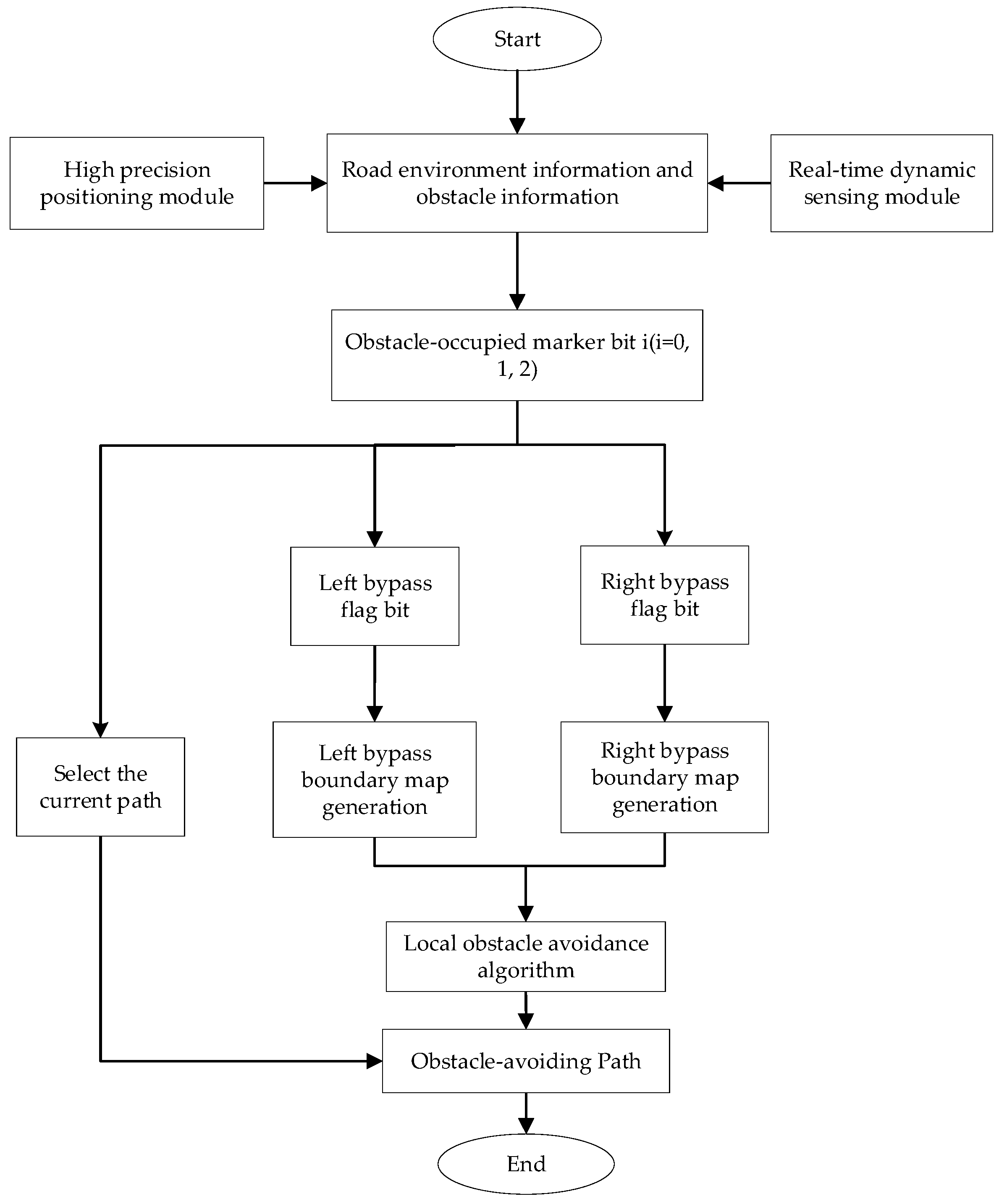
2. Local Path Generation Based on Spatial Perception

2.1. Dynamic Control Point Determination

Local obstacle avoidance path planning for intelligently driving sightseeing vehicles presents a nuanced challenge. Encountering obstacles necessitates the vehicle integrating global path data with real-time environmental inputs [29]. Informed by these combined insights, the vehicle then ascertains control points for immediate obstacle circumvention, facilitating the refinement and calibration of the local trajectory. This systematic approach ensures stable and safe navigation around impediments [30].

2.1.1. Acquisition of Global Path Points

The local path’s derivation is intrinsically linked to the global path. Hence, acquiring global path points becomes pivotal for establishing control points within the local obstacle avoidance trajectory. The procedure to shape the global path for the intelligent driving sightseeing vehicle unfolds in this manner: In specific contexts, the vehicle’s perception system processes data from an array of heterogeneous sensors. This fusion enhances both environmental perception accuracy and the quality of intelligent decision-making. This approach harnesses an ensemble of sensors, including LiDAR, cameras, and GNSS, among others, to glean real-time information on vehicle position, obstacle locales, and road specifics. Such data is then synergized to formulate high-fidelity maps. Subsequently, a secluded road is designated as the reference trajectory, with the sightseeing vehicle navigating its centerline at subdued speeds. Throughout this journey, the GNSS/GPS high-precision positioning module captures real-time coordinates of the road’s central path. The data amassed is fed into the Prescan 2019.2.0 software to devise a structured roadway. The Prescan software is capable of generating a comprehensive global map by utilizing the collected data. Subsequently, an integrated simulation is executed, intertwining Simulink and Prescan functionalities. Within the Prescan simulation interface, the sightseeing vehicle maintains a steady velocity along the road’s median, archiving its positional coordinates. These coordinates are subsequently relayed to Matlab, facilitating the fitting process and the computation of the road’s curvature.

The road centerline path, once fitted, is delineated by a series of discrete spatial points spaced 0.2 m apart. Each of these points is defined by its positional coordinates (X, Y) and accompanying curvature (ω). To elevate the precision of the local obstacle avoidance trajectory, the outset of each operational cycle pinpoints the point nearest to the vehicle’s center as the reference path’s commencement. Consequently, the subsequent 150 points from this origin form the reference trajectory. This reference trajectory, constituted by X(i), Y(i), and ω(i) for i ranging from 1 to 150, undergoes consistent updates in line with the vehicle’s advancement.

2.1.2. Determination of Control Points for Local Obstacle Avoidance Path

For the safe and comfortable execution of obstacle avoidance, it is imperative to institute a constraint on the spatial distance between the vehicle and the obstacles, known as the spatiotemporal safety constraint. Concurrently, ensuring the path’s smoothness and stability mandates restrictions on its curvature alterations. This restriction is termed the curvature constraint for obstacle avoidance. Considering both the vehicle’s spatial position and the spatial data of obstacles, dynamic control points are established by jointly considering spatiotemporal safety and curvature constraints. Figure 1 illustrates a straightforward lane-changing scenario for obstacle avoidance. Throughout this process, to prevent collisions, the intelligent driving vehicle must maintain the requisite safety distance. This ensures that the longitudinal distance between its current spatial position and that of nearby obstacles remains sufficiently expansive. Several assumptions are made for this analysis: (1) No obstacles exist on the neighboring lanes. (2) Obstacles ahead of the intelligent driving vehicle maintain a constant, lower speed. The longitudinal safety distance, often determined using TTC (time-to-collision) [31], serves as a measure for calculating the collision safety distance and assessing the safety level. This distance is influenced by the relative longitudinal velocity between the intelligent driving vehicle and the obstacle ahead [32,33,34]. Thus, the longitudinal safety distance between the vehicle’s real-time spatial position and the forward obstacle’s position can be denoted as $d_0$, and its value can be derived from Equation (1).

$$d_0=\left\{\begin{array}{c}\left(v_0-v_{ob}\right){\alpha }_0+l_0\\ l_0\end{array}\right.$$

(1)

where $l_0$ denotes the appropriate following distance between vehicles,$v_0$ signifies the current speed of the intelligent driving sightseeing vehicle, and $v_{ob}$ represents the speed of the obstacle ahead. The term ${\alpha }_0$ indicates the minimum safe time interval to avoid a collision.

To ensure trajectory curvature continuity while mitigating computational demands, we harness the features of B-spline curves. Specifically, these curves facilitate the translation of constraints on the trajectory curvature imposed by actuators into limitations regarding segment lengths and angles. Alongside the constraint of longitudinal safety distance for obstacle avoidance, these determinants collaboratively dictate the positioning of the B-spline curve control points. For a B-spline curve characterized by its linear segments, its maximum curvature, denoted as $k_{max}$, is steered by two pivotal parameters [35]: the segment length $d_1$ and the segment angle $\beta$. Within the context of the aforementioned obstacle avoidance lane-change scenario, $d_1$ stands for the obstacle avoidance curvature constraint distance. The relationship between $d_1$ and $\beta$ is shown in the control line segment model in Figure 2. As long as any two control line segments satisfy Equation (2), the curvature of the B-spline curve is guaranteed.

$$d_1⩾\frac{1}{6}\frac{\sin \beta }{{\kappa }_{max}}{\left(\frac{1-\mathrm{c}\mathrm{o}\mathrm{s}\beta }{8}\right)}^{-1.5}$$

(2)

The characteristics of Nth-degree B-spline curves vary with their degree. As the curve’s degree escalates, its derivatives’ order augments, leading to an increase in the zeros of the curve. This proliferation of zeros can result in a curve exhibiting multiple extrema, translating into more pronounced peaks and troughs. However, a curve with a diminished degree can more closely approximate its control points [36]. Given their second-order derivative continuity, cubic B-spline curves are optimal for trajectory planning. Specifically, quasi-uniform cubic B-spline curves, which typically necessitate at least four control points, are preferred to craft a seamless, smooth curve. The curve’s commencement in terms of position and direction is shaped by the initial three control points, whereas its termination is determined by the concluding three. To refine the curve’s contour, additional control points can be interspersed between these primary control points.

To facilitate a more fluid lane-changing maneuver for the intelligent driving sightseeing vehicle, the avoidance path is defined using a quasi-uniform cubic B-spline curve, delineated by six control points: $A_0,A_1,A_2,A_3,A_4,\mathrm{a}\mathrm{n}\mathrm{d}{A}_5$. Point $A_0$ corresponds to the center of the vehicle’s front end, marking the inception of the avoidance path. The real-time coordinates of $A_0$, designated as ${\left[x_0,y_0\right]}^T$, are procured through the onboard GNSS/GPS module. Conversely, point $A_5$ signifies the conclusion of the avoidance path, indicating that the vehicle has wholly circumvented the obstacle. The coordinates of $A_5$, represented as ${\left[x_5,y_5\right]}^T$, are ascertained based on the obstacle’s real-time spatial location. Assuming the distance between $A_0$ and $A_1$ mirrors that between $A_4$ and $A_5$, the positions of control points $A_1$ and $A_4$ can be determined via the control segment $d_2$. To ensure compliance with both avoidance safety and curvature continuity constraints, $d_2$ must adhere to the ensuing relationship:

$$d_2⩾\mathrm{m}\mathrm{a}\mathrm{x}(d_0,d_1)$$

(3)

For determining the positions of control points $A_1$ and $A_4$, the following methodology is adopted:

$$\left\{\begin{array}{c}{A}_1=\left[\begin{array}{c}{x}_1\\ y_1\end{array}\right]=\left[\begin{array}{c}{x}_0+d_{2}cos\left({\beta }_0\right)\\ y_0+d_{2}sin\left({\beta }_0\right)\end{array}\right]\\ A_4=\left[\begin{array}{c}{x}_4\\ y_4\end{array}\right]=\left[\begin{array}{c}{x}_{45}-d_{2}cos\left({\beta }_0\right)\\ y_{45}-d_{2}sin\left({\beta }_0\right)\end{array}\right]\end{array}\right.$$

(4)

The positions of control points $A_1$ and $A_4$ are influenced by ${\beta }_0$, the map’s heading angle, ascertainable in real-time via the GNSS/GPS module.

Upon establishing the positions of control points $A_1$ and $A_4$, the foundational shape of the B-spline curve emerges. For a refined, smoother, and local curve, additional control points, $A_2$ and $A_3$, are interpolated between $A_1$ and $A_4$. To preserve curvature continuity, an initial strategy positions $A_2$ and $A_3$ at the trisection points of the segment connecting $A_1$ to $A_4$. Control points $A_2$ and $A_3$ can be calculated using Equation (5).

$$\left\{\begin{array}{c}{A}_2=\left[\begin{array}{c}{x}_2\\ y_2\end{array}\right]=\left[\begin{array}{c}\raisebox{1ex}{$\left(2x_1+x_4\right)$}\!\left/ \!\raisebox{-1ex}{$3$}\right.\\ \raisebox{1ex}{$\left(2y_1+y_4\right)$}\!\left/ \!\raisebox{-1ex}{$3$}\right.\end{array}\right]\\ A_3=\left[\begin{array}{c}{x}_3\\ y_3\end{array}\right]=\left[\begin{array}{c}\raisebox{1ex}{$\left(x_1+2x_4\right)$}\!\left/ \!\raisebox{-1ex}{$3$}\right.\\ \raisebox{1ex}{$\left(y_1+{2y}_4\right)$}\!\left/ \!\raisebox{-1ex}{$3$}\right.\end{array}\right]\end{array}\right.$$

(5)

The preliminary control points, as derived for the quasi-uniform cubic B-spline curve, are depicted in Figure 3.

2.2. Dynamic Control Point Optimization

The quasi-uniform cubic B-spline curve’s six control points have been established, laying out an initial local obstacle avoidance path. Nonetheless, there’s potential for this path segment to veer too close to obstacles, which might divert it from the optimal trajectory. The inherent characteristics of B-spline curves mean local control point modifications will not alter the overall curve. By incorporating road data, the positions of control points $A_2$ and $A_3$ are adjusted, framing the path planning challenge in mathematical terms. To maintain the safety of the intelligent driving sightseeing vehicle during obstacle avoidance, considerations are made for both the timeliness and the stability of the maneuver. The distance $d_{obs}$ is used to determine whether the intelligent vehicle will collide with obstacles during the driving process. $d_{obs}$ represents the minimum gap from the obstacle’s center to the segment joining of $A_1$ and $A_4$, and gauges the risk of collision. The vehicle should adhere to the subsequent condition:

$$d_{obs}⩾(W+0.5)$$

(6)

where $W$ denotes the vehicle’s width. Accounting for the precision of the actual path-tracking algorithm, a buffer of 0.5 m is incorporated into the driving process. If $d_{obs}$ does not adhere to Equation (6), local refinements of the B-spline curve’s control points $A_2$ and $A_3$ become requisite. These control points are offset by a distance $d_4$ along the B-spline curve in the positive normal direction. $d_4$ is equal to half the vehicle’s width with an added minor margin, facilitating local path optimization. The determination of $d_4$ is equal to half the vehicle’s width with an added minor margin, facilitating local path optimization. The determination of

$$d_4=\left(W+0.5\right)-d_{obs}$$

(7)

2.3. Obstacle Avoidance Path Generation

Upon determining the dynamic control points, B-spline curves facilitate the creation of the local obstacle avoidance path via discrete interpolation. These curves, constructed from established control points, can employ either uniform or non-uniform parametric techniques. The methodology entails formulating expressions for the basis functions, followed by the assembly of diagonal matrices through the linear combination of these functions. This culminates in the production of a smooth curve [37].

Consider a scenario where we have a total of n + 1 control points, represented as $P_0,P_1,P_2,\dots ,P_n$. These control points serve to delineate the direction and boundary constraints of the spline curve. Based on these control points, the B-spline curve can be defined as follows:

$$P\left(u\right)=\left[P_0{P}_1{P}_2\dots P_n\right]\left[\begin{array}{c}{B}_{0,k}\left(u\right)\\ B_{1,k}\left(u\right)\\ ⋮\\ B_{n,k}\left(u\right)\end{array}\right]=\sum _{i=0}^n{P}_i{B}_{i,k}(u)$$

(8)

where $B_{i,k}\left(u\right)$ represents the $i$-th $k$-th-order B-spline basis function, $P_i$ is a control point, and $k\ge 1$. The variable $u$ is the independent variable. The basis function $B_{i,k}\left(u\right)$ is derived from the De Boor–Cox recursion formula [38]

$$B_{i,k}\left(u\right)=\left\{\begin{array}{ll}\left\{\begin{array}{ll}1,& u_i\le u<u_{\dot{i}+1}\\ 0,& others\end{array},\right.& k=1\\ \frac{u-u_i}{u_{i+k-1}-u_i}{B}_{i,k-1}\left(u\right)+\frac{u_{i+k}-u}{u_{i+k}-u_{i+1}}{B}_{i+1,k-1}\left(u\right),& k\ge 2\end{array}\right.$$

(9)

Conventionally, the indeterminate form $\raisebox{1ex}{$0$}\!\left/ \!\raisebox{-1ex}{$0$}\right.$ is defined as 0. Here, $u_i$ represents a set of continuously varying values known as knot vectors, with the initial and final values typically defined as 0 and 1. The sequence of $u_i$ can be expressed as $\left[u_0{u}_1\dots u_k,u_{k+1},\dots ,u_n,u_{n+1},\dots ,u_{n+k}\right]$.

B-spline curves, as categorized by the distribution of knot vectors, fall into two main types: uniform B-spline curves and quasi-uniform B-spline curves [39]. The latter, with its non-uniform parameter distribution, is distinguished by its capacity for greater shape flexibility. This makes it especially adept at adapting to intricate road conditions and meeting obstacle avoidance criteria. Further enhancing their utility, quasi-uniform B-spline curves retain the characteristics of Bezier curves at their extremities. This ensures that the tangent at the endpoints matches the line joining the last two endpoints, thereby guaranteeing the continuity of the curvature in the obstacle avoidance trajectory.

Drawing from the global path, alongside real-time vehicular positioning and obstacle perception data, it is feasible to ascertain and refine the control points of the B-spline curve in a localized context. This culminates in the final set of control points. Interpolation conducted on these six terminal points facilitates the creation of a smooth B-spline curve. To forge a real-time, local obstacle-avoidance trajectory, this curve undergoes a process of discretization. It is pivotal to synchronize the discretization sampling time with that used to derive the global path. Subsequently, the resulting discrete spatial coordinates compose the definitive local obstacle-avoidance spatiotemporal trajectory.

Figure 4 illustrates the local obstacle-avoidance trajectory, derived from the finalized control points. Notably, this trajectory adheres to stringent safety standards throughout the driving process and aligns with vehicular kinematic constraints. This alignment guarantees a minimal variation in curvature during obstacle evasion.

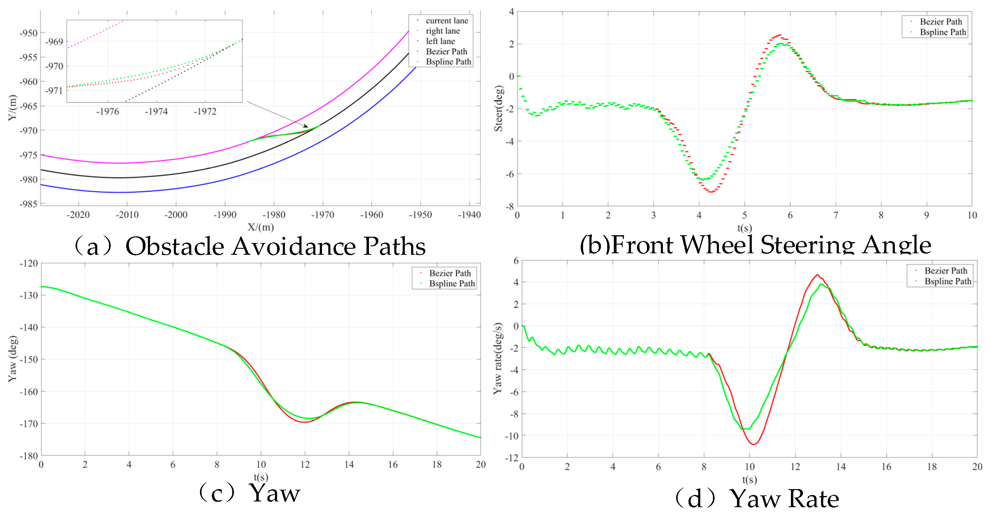
3. Simulation Analysis

3.1. Model Construction

To assess the efficacy of the local obstacle-avoidance algorithm, we monitored paths generated by the algorithm on roads exhibiting varied spatial features. Within the Prescan software, we constructed three road types, each distinct in spatial characteristics: straight roads, sharply curved roads, and continuously curved roads. These road categories encompass a broad range of practical driving scenarios, showcasing the algorithm’s versatility. Leveraging the Simulink(R2021a)/Prescan 2019.2.0 software, we captured the coordinates of the global path points across these road types. Subsequently, a path-tracking simulation model was established using Simulink(R2021a)/Carsim 2019.0 software.

For our simulation model, we opted for the B-class rear-wheel-drive electric vehicle from the Carsim dataset. This selection was based on its close alignment with the parameters of the actual tested intelligent driving sightseeing vehicle. All model parameters were tailored to reflect the real vehicle specifications, and the details are presented in Supplementary Materials. Within this simulation framework, the primary input variable for the test vehicle is the front wheel steering angle. Conversely, the key output variables encompass the actual vehicle speed, front wheel steering angle, yaw angle, and yaw rate, among others.

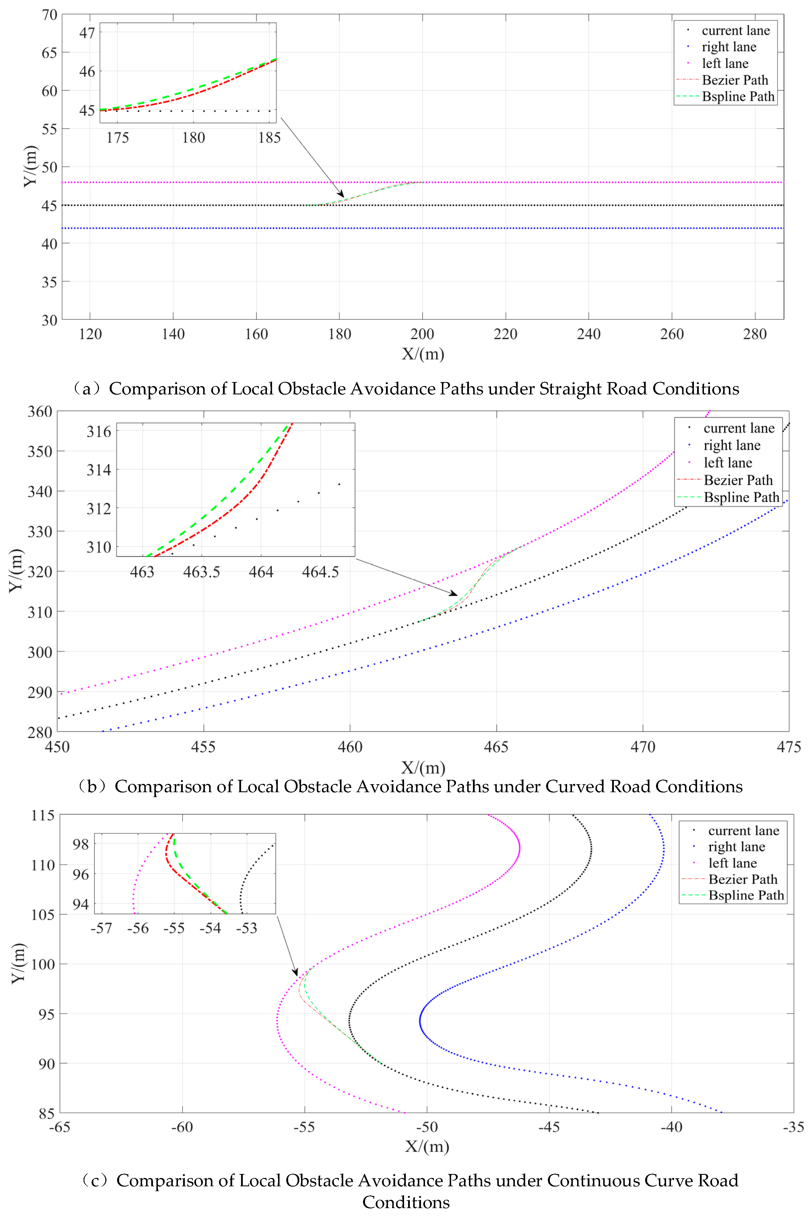
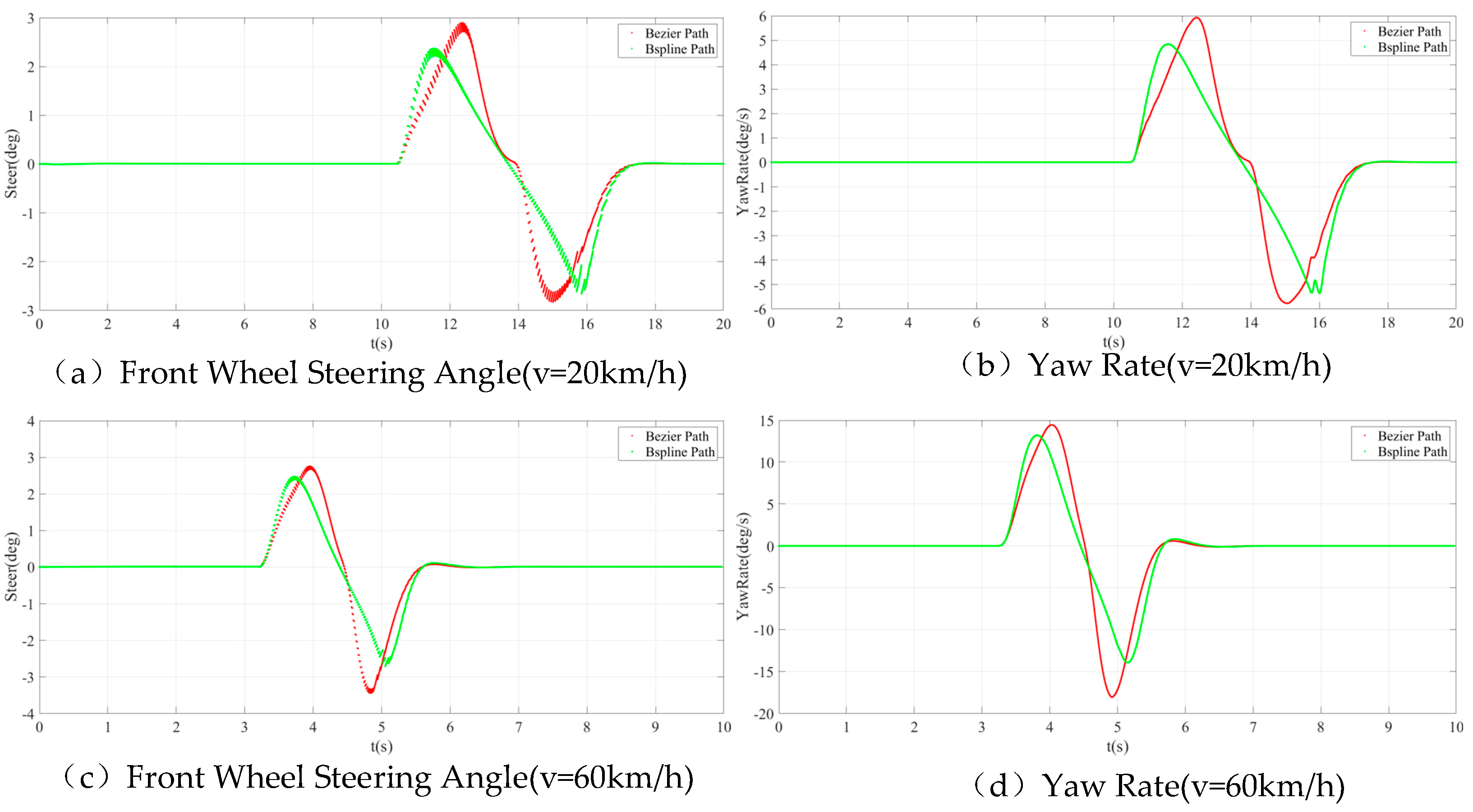
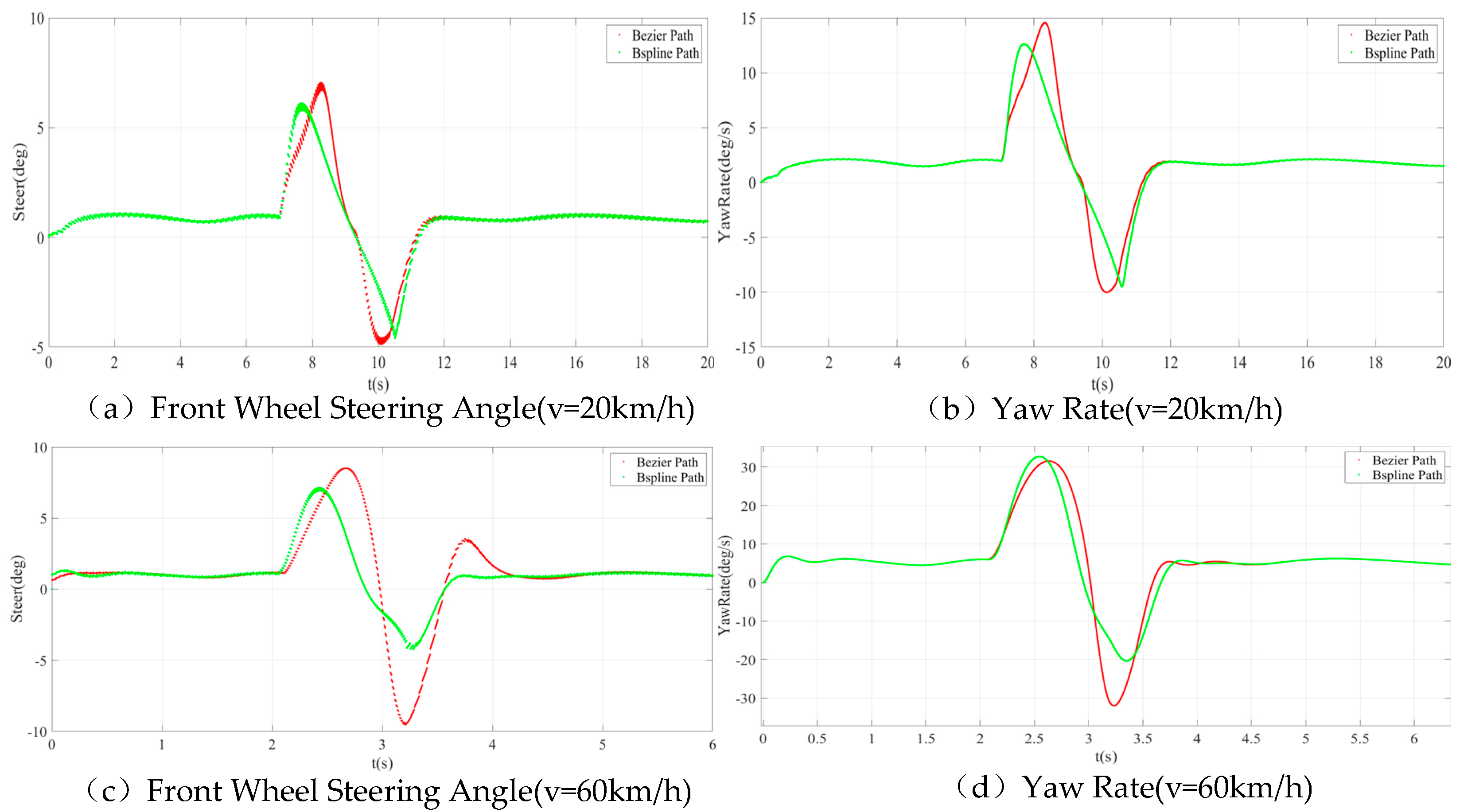
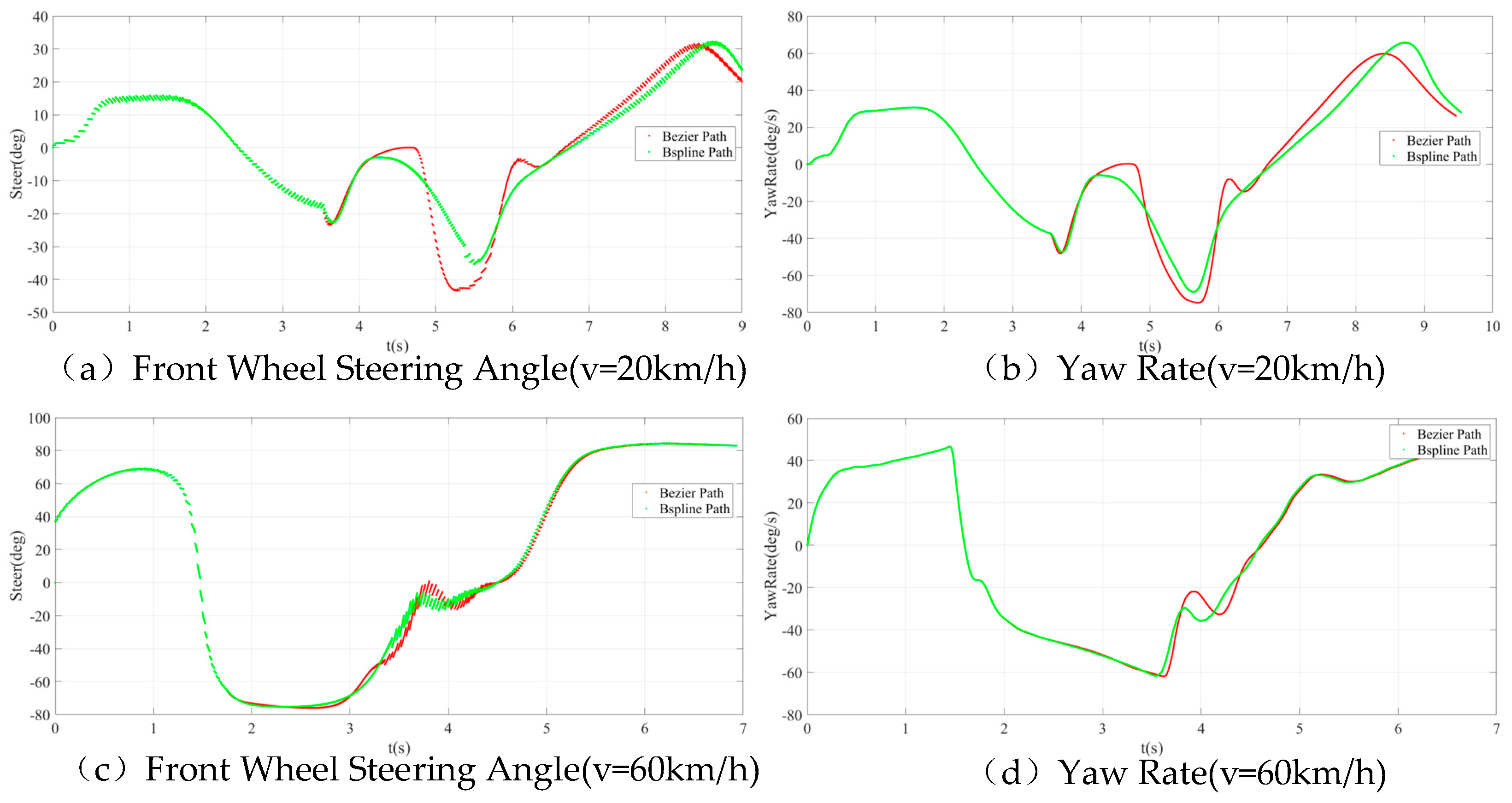
3.2. Simulation Result

Considering three distinct spatial road characteristics, we factored in vehicle data, road specifics, and obstacle details to determine the control points for the local avoidance algorithm. Following this, we conducted curve discretization interpolation to devise the corresponding local avoidance path. For comparative analysis, we also generated a local avoidance path employing Bézier curves.

As can be seen from Figure 5, local avoidance paths are illustrated for three distinct spatial road features. The primary lane of the intelligent driving sightseeing vehicle is marked in black, while neighboring lanes are shown in blue. The paths determined by the conventional Bezier curve are represented by the red line, whereas the B-spline curve paths are delineated by the green line. Across all road variations, both the B-spline and Bezier curves adeptly design local avoidance trajectories. It is worth noting that paths from the B-spline curve display a more fluid transition with milder curvature changes. This distinction is especially evident on roads characterized by pronounced curves or continuous bends, underscoring the B-spline curve’s enhanced capability for smooth obstacle circumvention.

In the path-tracking model, the intelligent driving sightseeing vehicle navigates two distinct obstacle avoidance paths on roads characterized by varying spatial features, doing so at two separate speeds of 20 km/h and 60 km/h. Utilizing the Carsim simulation platform, real-time metrics for front wheel steering angles and vehicle yaw angles are captured. This data serves as a benchmark to assess the fluidity of the obstacle avoidance paths. Figure 6, Figure 7 and Figure 8 depict the corresponding front wheel steering angles and vehicle yaw angles for the three specific road conditions.

As can be seen from Figure 6, real-time variations in the vehicle’s front wheel steering angles and yaw angles emerge when traversing a straight road. When following the Bezier curve for obstacle avoidance, the maximum steering angles of the front wheel peak at 2.9° and 3.5°, with the maximum yaw angle rates of change reaching 6 deg/s and 17 deg/s, respectively. Conversely, when navigating via the refined B-spline curve obstacle avoidance method, the maximum steering angles of the front wheel are limited to 2.9° and 2.7°, and the peak yaw angle rate of change stands at 5.5 deg/s and 13 deg/s, respectively. Such observations underscore that on straight roads, trajectories designed using the B-spline curve algorithm manifest inherently smoother dynamics.

As can be seen from Figure 7, there are notable variations in the vehicle’s front wheel steering angles and yaw angles on a curved road. When the vehicle follows the Bezier curve obstacle avoidance path, the maximum steering angles of the front wheel measure at 7° and 9.5°, while the maximum yaw angle rate of changes are 14.8 deg/s and 30 deg/s, respectively. On the other hand, when utilizing the B-spline curve obstacle avoidance method, the steering angles of the front wheel peak at 6.2° and 7°, with the highest yaw angle rates of change being 12 deg/s and 32 deg/s, respectively. These findings suggest that on curved roads, the intelligent sightseeing vehicle demonstrates a more fluid driving experience when following the trajectory crafted using the B-spline curve algorithm.

As can be seen from Figure 8, the vehicle’s front wheel steering angle and its heading angle exhibit distinct dynamics under continuous curve road conditions. When adhering to the Bezier curve obstacle avoidance trajectory, the front wheel reaches steering angles of 43° and 78° at their peak. Simultaneously, the most pronounced changes in the vehicle’s heading angle are 78 deg/s and 62 deg/s, respectively. Conversely, following the refined B-spline curve obstacle avoidance trajectory results in maximal steering angles of 35° and 77° for the front wheel, and heading angle change rates peaking at 70 deg/s and 62 deg/s. These data, especially when observed in rapidly altering curvatures of continuous curve roads, reaffirm the heightened smoothness inherent in the trajectories generated by the improved B-spline curve method.

4. On-Vehicle Experiment

The intelligent sightseeing car deployed in our real-world experiments originates from Liuzhou Wuling Automobile Industry Corporation Limited. This particular vehicle boasts a robust and dependable wire-controlled chassis, seamlessly integrating steering, throttle, and braking controls, all managed via signals from its autonomous driving domain controller. The embedded autonomous driving software system of the vehicle is multi-faceted, encompassing a high-precision map module, a localization module, a perception module, a decision-making module, a planning module, and a control module. Ensuring efficient inter-module communication, these elements utilize the ROS communication protocol and are meticulously crafted using the C++ programming language. The aesthetics and design of this advanced sightseeing vehicle are showcased in Figure 9.

The planning module of the intelligent sightseeing car initiates its process by leveraging a lane-following map for global path planning, which delineates the vehicle’s overarching route. This module then makes judicious decisions based on real-time spatial perception of obstacles and the associated lane occupation flag, denoted as “i”. This flag aids in determining whether the vehicle should navigate to the left or right side of an obstacle. Specifically, the values of “i” can be 0, 1, or 2, which correspond to the middle lane, left lane, and right lane, respectively. By employing the local obstacle avoidance algorithm, the module crafts a local obstacle avoidance path attuned to the prevailing road circumstances. Figure 10 elucidates the algorithmic procedure underpinning this planning module.

Experiments using the real vehicle were conducted on a closed two-way lane within the campus. This lane is characterized by both straight and curved sections. Given the constraints of the straight section’s length in the test area and in the interest of safety, the vehicle’s driving speed was capped at 12 km/h. The lane itself spans a width of 3.5 m, and with the inclusion of curbing on each side, the effective width extends to 4.0 m. In addressing the varied spatial features of the road, the planning module employed both the improved B-spline curve and the Bezier curve for generating obstacle avoidance trajectories. Comprehensive results from these real-world tests are depicted in Figure 11 and Figure 12. These figures present the coordinates of the obstacle avoidance path points and relevant data, including front wheel angles, yaw angles, and yaw rates for the various road conditions encountered.

As can be seen from Figure 11a and Figure 12a, both algorithms present similar trajectories up until the point they encounter obstacles. Upon confronting these obstacles, both methodologies successfully devise logical obstacle avoidance paths. Nevertheless, the trajectory produced by the B-spline curve demonstrates a marked improvement in smoothness compared to that of the Bezier curve. Delving deeper into Figure 11b–d and Figure 12b–d, it becomes evident that the B-spline curve fitting algorithm leads to fewer fluctuations in both the front wheel angle and the yaw angle. This implies a more consistent and stable performance by the intelligent sightseeing vehicle when navigating around obstacles, regardless of whether the road conditions are straight or curved.

5. Conclusions

This research employs a high-precision positioning module and a real-time perception module to acquire road environment information in specific scenarios. Considering spatiotemporal safety constraints and obstacle avoidance curvature constraints, it determines control points for the local obstacle avoidance path, which is discretely interpolated using B-spline curves. Comparative analysis with paths generated using the Bezier curve algorithm, conducted through simulation and real vehicle experiments, illustrates that in each road scenario, the local obstacle avoidance algorithm produces smoother obstacle avoidance paths. Minimal variations in the front-wheel steering angle and yaw angle of the intelligent driving sightseeing vehicle indicate enhanced vehicle stability.

When integrated with geographic information fusion, the algorithm demonstrates the potential to elevate path planning precision, strengthen environmental perception capabilities, optimize the route selection, and enhance the real-time responsiveness of path updates. It is noteworthy, however, that due to constraints within the real-world testing environment for vehicular experiments, the local obstacle avoidance algorithm has yet to undergo testing in high-speed scenarios. Future research endeavors will encompass testing the algorithm in high-speed contexts and its application across diverse environments, further validating its performance.

References

1. Li, Y.; Fan, J.; Liu, Y.; Wang, X. Path Planning and Path Tracking for Autonomous Vehicle Based on MPC with Adaptive Dual-Horizon-Parameters. Int. J. Automot. Technol. 2022, 23, 1239–1253. [Google Scholar] [CrossRef]
2. Xiong, L.; Fu, Z.; Zeng, D.; Qian, Z.; Leng, B. A Path Planning and Tracking Framework Based on Model Predictive Control for Autonomous Vehicle Obstacle Avoidance. In Proceedings of the 27th Symposium of the International Association of Vehicle System Dynamics, IAVSD 2021, Virtual, 17–19 August 2021; pp. 1137–1143. [Google Scholar]
3. Tang, P.; Yang, R.; Ni, X.; Zhao, H.; Xu, F. Research on a lightweight unmanned sightseeing vehicle frame based on multi-condition and multi-objective optimization. Adv. Mech. Eng. 2022, 14, 16878132221131748. [Google Scholar] [CrossRef]
4. Jiao, M.; Song, Y. Path Planning for Unmanned Campus Sightseeing Vehicle with Linear Temporal Logic. In Proceedings of the 2018 Chinese Intelligent Systems Conference, Singapore, 23 December 2019; pp. 329–337. [Google Scholar]
5. Wang, M.-L.; Luo, J.-H.; Yang, Y.; Liu, T.; Li, Y.-F. Application Analysis of GIS on UGV Autonomous Navigation. Beijing Ligong Daxue Xuebao/Trans. Beijing Inst. Technol. 2019, 39, 907–911. [Google Scholar] [CrossRef]
6. Lim, K.-I.; Oh, J.-S.; Lee, J.-U.; Kim, J.-H. Development of an intelligent cruise control using path planning based on a geographic information system. J. Inst. Control Robot. Syst. 2015, 21, 217–223. [Google Scholar] [CrossRef]
7. Choi, Y.-G.; Lim, K.-I.; Kim, J.-H. Lane change and path planning of autonomous vehicles using GIS. In Proceedings of the 12th International Conference on Ubiquitous Robots and Ambient Intelligence, URAI 2015, Goyang City, Republic o Korea, 28–30 October 2015; pp. 163–166. [Google Scholar]
8. Hosseinyalamdary, S.; Balazadegan, Y.; Toth, C. Tracking 3D Moving Objects Based on GPS/IMU Navigation Solution, Laser Scanner Point Cloud and GIS Data. ISPRS Int. J. Geo-Inf. 2015, 4, 1301–1316. [Google Scholar] [CrossRef]
9. Zhu, H.; Fu, M.; Yang, Y.; Wang, X.; Wang, M. A path planning algorithm based on fusing lane and obstacle map. In Proceedings of the 2014 17th IEEE International Conference on Intelligent Transportation Systems, ITSC 2014, Qingdao, China, 8–11 October 2014; pp. 1442–1448. [Google Scholar]
10. Wang, M.-L.; Pan, Y.-H. Research on optimal path planning with constraints based on GIS. Beijing Ligong Daxue Xuebao/Trans. Beijing Inst. Technol. 2016, 36, 851–856; 861. [Google Scholar] [CrossRef]
11. Fu, M.; Song, W.; Yi, Y.; Wang, M. Path Planning and Decision Making for Autonomous Vehicle in Urban Environment. In Proceedings of the 18th IEEE International Conference on Intelligent Transportation Systems, ITSC 2015, Gran Canaria, Spain, 15–18 September 2015; pp. 686–692. [Google Scholar]
12. Yang, F.; Zhu, Z.; Gong, X.-J.; Liu, J.-L. Real-time dynamic obstacle detection and tracking using 3D Lidar. Zhejiang Daxue Xuebao (Gongxue Ban)/J. Zhejiang Univ. (Eng. Sci.) 2012, 46, 1565–1571. [Google Scholar] [CrossRef]
13. Zhong, M.; Wu, Y.; Wan, F.; Fu, Q. Research on Dynamic Path Planning of Internet of Vehicles Based on Edge Computing. In Proceedings of the 2nd International Conference on Networking, Communications and Information Technology, NetCIT 2022, Virtual, 26–27 December 2022; pp. 453–457. [Google Scholar]
14. Shi, S.; Cui, J.; Jiang, Z.; Yan, Z.; Xing, G.; Niu, J.; Ouyang, Z. VIPS: Real-Time Perception Fusion for Infrastructure-Assisted Autonomous Driving. In Proceedings of the 28th ACM Annual International Conference on Mobile Computing and Networking, MobiCom 2022, Sydney, NSW, Australia, 17–21 October 2202; pp. 133–146. [Google Scholar]
15. Gamerdinger, J.; Teufel, S.; Volk, G.; Bringmann, O. CoLD Fusion: A Real-time Capable Spline-based Fusion Algorithm for Collective Lane Detection. In Proceedings of the 34th IEEE Intelligent Vehicles Symposium, IV 2023, Anchorage, AK, USA, 4–7 June 2023; IEEE Intelligent Transportation Systems Society (ITSS): Piscataway, NJ, USA, 2023. [Google Scholar]
16. Gonzalez, D.; Perez, J.; Milanes, V.; Nashashibi, F. A review of motion planning techniques for automated vehicles. IEEE Intell. Transp. Syst. Mag. 2016, 17, 1135–1145. [Google Scholar] [CrossRef]
17. Chen, J.; Zhao, Y.; Xu, X. Improved RRT-Connect Based Path Planning Algorithm for Mobile Robots. IEEE Access 2021, 9, 145988–145999. [Google Scholar] [CrossRef]
18. Tang, X.; Zhu, Y.; Jiang, X. Improved a-star algorithm for robot path planning in static environment. In Proceedings of the 2020 International Conference on Communications, Information System and Software Engineering, CISSE 2020, Guangzhou, China, 18–20 December 2020. [Google Scholar]
19. Claussmann, L.; Revilloud, M.; Gruyer, D.; Glaser, S. A Review of Motion Planning for Highway Autonomous Driving. IEEE Trans. Intell. Transp. Syst. 2020, 21, 1826–1848. [Google Scholar] [CrossRef]
20. Kang, J.-G.; Lim, D.-W.; Choi, Y.-S.; Jang, W.-J.; Jung, J.-W. Improved RRT-connect algorithm based on triangular inequality for robot path planning. Sensors 2021, 21, 333. [Google Scholar] [CrossRef] [PubMed]
21. Zheng, L.; Zeng, P.; Yang, W.; Li, Y.; Zhan, Z. Bézier curve-based trajectory planning for autonomous vehicles with collision avoidance. IET Intell. Transp. Syst. 2020, 14, 1882–1891. [Google Scholar] [CrossRef]
22. Wang, Y.; Wei, C.; Ma, L. Dynamic Lane-changing Trajectory Planning Model for Intelligent Vehicle Based on Quadratic Programming. Zhongguo Gonglu Xuebao/China J. Highw. Transp. 2021, 34, 79–94. [Google Scholar] [CrossRef]
23. Han, L.; Yashiro, H.; Nejad, H.T.N.; Do, Q.H.; Mita, S. Bézier curve based path planning for autonomous vehicle in urban environment. In Proceedings of the 2010 IEEE Intelligent Vehicles Symposium, IV 2010, La Jolla, CA, USA, 21–24 June 2010; pp. 1036–1042. [Google Scholar]
24. Chen, C.; He, Y.; Bu, C.; Han, J.; Zhang, X. Quartic Bézier curve based trajectory generation for autonomous vehicles with curvature and velocity constraints. In Proceedings of the 2014 IEEE International Conference on Robotics and Automation (ICRA), Hong Kong, China, 31 May–7 June 2014; pp. 6108–6113. [Google Scholar]
25. Donatelli, M.; Giannelli, C.; Mugnaini, D.; Sestini, A. Curvature continuous path planning and path finding based on PH splines with tension. CAD Comput. Aided Des. 2017, 88, 14–30. [Google Scholar] [CrossRef]
26. Yamamoto, M.; Iwamura, M.; Mohri, A. Quasi-time-optimal motion planning of mobile platforms in the presence of obstacles. Proc.–IEEE Int. Conf. Robot. Autom. 1999, 4, 2958–2963. [Google Scholar]
27. Xu, W.; Yang, Y.; Yu, L.-T.; Zhu, L. A global path planning algorithm based on improved RRT. Kongzhi Yu Juece/Control Decis. 2022, 37, 829–838. [Google Scholar] [CrossRef]
28. Elbanhawi, M.; Simic, M.; Jazar, R. Randomized Bidirectional B-Spline Parameterization Motion Planning. IEEE Trans. Intell. Transp. Syst. 2016, 17, 406–419. [Google Scholar] [CrossRef]
29. Wang, P.; Yang, J.; Zhang, Y.; Wang, Q.; Sun, B.; Guo, D. Obstacle-Avoidance Path-Planning Algorithm for Autonomous Vehicles Based on B-Spline Algorithm. World Electr. Veh. J. 2022, 13, 233. [Google Scholar] [CrossRef]
30. Liu, H.; Li, X.; Fan, M.; Wu, G.; Pedrycz, W.; Suganthan, P.N. An Autonomous Path Planning Method for Unmanned Aerial Vehicle based on A Tangent Intersection and Target Guidance Strategy. IEEE Trans. Intell. Transp. Syst. 2020, 23, 3061–3073. [Google Scholar] [CrossRef]
31. Li, Z.; Li, J.; Wang, W. Path Planning and Obstacle Avoidance Control for Autonomous Multi-Axis Distributed Vehicle Based on Dynamic Constraints. IEEE Trans. Veh. Technol. 2023, 72, 4342–4356. [Google Scholar] [CrossRef]
32. Wang, S.Z.; Xu, W. Safe Distance Model for Control of Vehicle Emergency Collision Avoidance. Int. J. Veh. Struct. Syst. 2021, 13, 598–603. [Google Scholar] [CrossRef]
33. Zhang, R.; Li, K.; Wu, Y.; Zhao, D.; Lv, Z.; Li, F.; Chen, X.; Qiu, Z.; Yu, F. A Multi-Vehicle Longitudinal Trajectory Collision Avoidance Strategy Using AEBS with Vehicle-Infrastructure Communication. IEEE Trans. Veh. Technol. 2022, 71, 1253–1266. [Google Scholar] [CrossRef]
34. Zhao, L.; Zhang, D.; Wang, H.; Chen, W.; Wang, Q.; Zhu, M. Study on Longitudinal Collision Avoidance with Human-machine Cooperation Based on Improved Safety Distance Model. Qiche Gongcheng/Automot. Eng. 2021, 43, 588–600. [Google Scholar]
35. McNaughton, M.; Urmson, C.; Dolan, J.M.; Lee, J.-W. Motion planning for autonomous driving with a conformal spatiotemporal lattice. In Proceedings of the 2011 IEEE International Conference on Robotics and Automation, ICRA 2011, Shanghai, China, 9–13 May 2011; pp. 4889–4895. [Google Scholar]
36. Maekawa, T.; Noda, T.; Tamura, S.; Ozaki, T.; Machida, K.-i. Curvature continuous path generation for autonomous vehicle using B-spline curves. CAD Comput. Aided Des. 2010, 42, 350–359. [Google Scholar] [CrossRef]
37. Lu, E.; Ruan, Q.; Liu, Y.; Wang, F.; Lin, W.; Dong, B. Obstacle Avoidance Path Planning for Intelligent Forklift Truck Based on Dynamic Identification Zone and B-spline Curve. Nongye Jixie Xuebao/Trans. Chin. Soc. Agric. Mach. 2019, 50, 359–366. [Google Scholar] [CrossRef]
38. Cao, H.; Zoldy, M. Implementing B-Spline Path Planning Method Based on Roundabout Geometry Elements. IEEE Access 2022, 10, 81434–81446. [Google Scholar] [CrossRef]
39. Nguyen, N.T.; Gangavarapu, P.T.; Kompe, N.F.; Schildbach, G.; Ernst, F. Navigation with Polytopes: A Toolbox for Optimal Path Planning with Polytope Maps and B-spline Curves. Sensors 2023, 23, 3532. [Google Scholar] [CrossRef] [PubMed]
Figure 1. Obstacle safety distance.
Applsci 13 11183 g001
Figure 2. Control line segment model.
Applsci 13 11183 g002
Figure 3. Illustration of B-spline curve control points.
Applsci 13 11183 g003
Figure 4. Local obstacle avoidance path.
Applsci 13 11183 g004
Figure 5. Comparison of local obstacle avoidance paths under three different conditions.
Applsci 13 11183 g005
Figure 6. Data comparison under straight road conditions.
Applsci 13 11183 g006
Figure 7. Data comparison under curved road conditions.
Applsci 13 11183 g007
Figure 8. Data comparison under continuous curve road conditions.
Applsci 13 11183 g008
Figure 9. Physical image of the intelligent autonomous sightseeing vehicle.
Applsci 13 11183 g009
Figure 10. Algorithm flowchart of the planning module.
Applsci 13 11183 g010
Figure 11. Data comparison of real vehicle under straight road conditions.
Applsci 13 11183 g011
Figure 12. Data comparison of real vehicle under curved road conditions.
Applsci 13 11183 g012
Disclaimer/Publisher’s Note: The statements, opinions and data contained in all publications are solely those of the individual author(s) and contributor(s) and not of MDPI and/or the editor(s). MDPI and/or the editor(s) disclaim responsibility for any injury to people or property resulting from any ideas, methods, instructions or products referred to in the content.